DEEP PREDICTION OF INVESTOR INTEREST: A SUPERVISED CLUSTERING APPROACH - arXiv.org
←
→
Page content transcription
If your browser does not render page correctly, please read the page content below
D EEP PREDICTION OF INVESTOR INTEREST:                                             A SUPERVISED
                                                                                CLUSTERING APPROACH

                                                                                                A P REPRINT

                                                                        Baptiste Barreau1, 2 , Laurent Carlier2 , and Damien Challet1
                                         1
                                             Chair of Quantitative Finance, MICS Laboratory, CentraleSupélec, Université Paris-Saclay, Gif-sur-Yvette, France
arXiv:1909.05289v3 [cs.LG] 26 Feb 2021

                                             2
                                             BNP Paribas Corporate & Institutional Banking, Global Markets Data & Artificial Intelligence Lab, Paris, France
                                                                     1
                                                                       {baptiste.barreau, laurent.carlier}@bnpparibas.com
                                                                              1
                                                                                damien.challet@centralesupelec.fr}

                                                                                               A BSTRACT
                                                    We propose a novel deep learning architecture suitable for the prediction of investor interest for a
                                                    given asset in a given time frame. This architecture performs both investor clustering and modelling
                                                    at the same time. We first verify its superior performance on a synthetic scenario inspired by real
                                                    data and then apply it to two real-world databases, a publicly available dataset about the position of
                                                    investors in Spanish stock market and proprietary data from BNP Paribas Corporate and Institutional
                                                    Banking.

                                         Keywords investor activity prediction, deep learning, neural networks, mixture of experts, clustering

                                         1       Introduction

                                         Predicting investor activity is a challenging problem in Finance. The basic problem can be stated as follows: given many
                                         thousands of assets and many thousands of investors, predict which investors will be interested in buying/selling which
                                         assets in the next (short) time period. What makes this problem difficult is the large heterogeneity of both investors and
                                         assets, compounded by the non-stationary nature of markets and investors and the limited time over which predictions
                                         are relevant.
                                         Ad-hoc methods are surprisingly efficient at clustering investors according to their trades in a single asset [Tumminello
                                         et al., 2012]. In addition, clusters of investors determined for several assets separately have a substantial overlap
                                         [Baltakys et al., 2018], which shows that one may be able to cluster investors for more than a few assets at a time. The
                                         activity of a given cluster may systematically depend on the previous activity of some clusters, which can then be used
                                         to predict the investment flow of investors [Challet et al., 2018]. Here, we leverage deep learning to train a single neural
                                         network on all the investors and all the assets of a given market and give temporal predictions for each investor.
                                         The heterogeneity of investors translates into a heterogeneity of investment strategies [Tumminello et al., 2012,
                                         Musciotto et al., 2018]: for the same set of information, e.g., financial and past activity indicators, investors can take
                                         totally different actions. Take for instance the case of an asset whose price has just decreased: some investors will buy it
                                         because they have positive long-term price increase expectations and thus are happy to be able to buy this asset at a
                                         discount; reversely, some other investors will interpret the recent price decrease as indicative of the future trend or risk
                                         and refrain from buying it.
                                         Formally, in our setting, a strategy f is a mapping from current information x to expression of interest to buy and/or
                                         sell a given asset, encoded by a categorical variable y: f : x 7→ y. We call here D = {fk : x 7→ y}k the set of all
                                         the investment strategies that an investor may follow. Unsupervised clustering methods suggest that the number of
                                         different strategies that describe investors’ decisions is finite [Musciotto et al., 2018]. We therefore expect our dataset
                                         to have a finite number K of clusters of investors, each following a given investment strategy fk . Consequently, we
                                         expect D to be such that |D| = K, i.e. D = {fk : x 7→ y}k=1,··· ,K . Alternatively, D can be thought of as the set
                                         of distinguishable strategies, which may be smaller than the total number of strategies and which may therefore be
Deep prediction of investor interest: a supervised clustering approach A P REPRINT
considered as an effective set of strategies. At any rate, a suitable algorithm to solve our problem therefore needs to be
able to infer the set of investment strategies D.
A simple experiment shows how investors differ. We first transform BNP Paribas CIB bonds’ Request for Quotation
(RFQ) database, along with market data and categorical information related to the investors and bonds, into a dataset of
custom-made, proprietary features describing the investors’ interactions with all the bonds under consideration. This
dataset is built so that each row can be mapped to a triplet (Investor, Financial Product, Date). This structure allows us,
for a given investor and at a given date, to provide probabilities of interest in buying and/or selling a given financial
product in a given timeframe. As the final decision following an RFQ is not always known, we consider the RFQ itself
as the signal of interest in a product. Consequently, we consider a given day to be a positive event for a given investor
and a given financial product when the investor actually signalled his interest in that product in a window of 5 business
days around that day. The reason is twofold: first because bonds are by essence illiquid financial products and second
because this increases the proportion of positive events.
At each date, negative events are randomly sampled in the (Investor, Financial Product) pairs that were observed as
positive events in the past and that are not positive at this date. Using this dataset, we conduct an experiment to illustrate
the non-universality of investors, i.e. the fact that investors have distinct investment strategies. The methodology of this
experiment is reminiscent of the one used in Sirignano and Cont [2018] to study the universality of equity limit order
books.
Figure 1: Universality matrix of investors’ strategies: the y-axis shows investors’ sector used to train a gradient boosting
model while the x-axis shows investors’ sector on which predictions are made using the model indicated on y-axis.
Scores are average precision, macro-averaged over classes and expressed in percentages.
We use a dataset constructed as described above with five months of bonds’ RFQ data. We split this dataset into
many subsets according to the investors’ business sector, e.g. one of these subset contains investors coming from the
Insurance sector only. We consider here only the sectors with a sufficient amount of data samples to train and test a
model. The remaining sectors are grouped together under the Others flag. Note that this flag is mainly composed of
Corporate sectors, such as car industry, media, technology, telecommunications. . . For each sector, some of the latest
data is held out, and a gradient boosting model is trained on the remaining data. This model is then used for prediction
on the held-out data of the model’s underlying sector, and for all the other sectors as well. For comparison purposes, an
aggregated model using all sectors at once is also trained and tested in the same way.
Because classes are unbalanced, we compute the average precision score of the obtained results, as advised by Davis
and Goadrich [2006], macro-averaged over all the classes, which yields the universality matrix shown in Fig. 1. The
y-axis labels the sector used for training, and the x-axis is the section on which the predictions are made.
We observe that some sectors are inherently difficult to predict, even when calibrated on their data only — this is the
case for Asset Managers of Private Banks and Pension Funds. On the contrary, some sectors seem to be relatively
easy to predict, e.g. Broker Dealers and, to some extent, Central Banks. Overall, we note that there is always some
degree of variability of the scores obtained by a given model — no universal model gives good predictions for all the
sectors of activity. Thus follows the non-universality of clients. In addition, it is worth noting that the aggregated model
2Deep prediction of investor interest: a supervised clustering approach A P REPRINT
Figure 2: Global architecture of an ExNet
obtained better performance on some sectors than the models trained on these sectors’ data only. As a consequence, a
suitable grouping of sectors would improve predictions for some sectors. This observation is in agreement with the
above K-investment strategies hypothesis.
Following on these hypotheses, this work leverages deep learning both to uncover the structure of similarity between
investors, namely the K clusters, or strategies, and to make relevant predictions using each inferred clusters. The
advantage of deep learning lies in the fact that it allows to solve both of these tasks at once, and thereby unveils the
structure of investors that most closely corresponds to their trading behaviour in a self-consistent way.
2 Related work
This work finds its roots in mixture-of-experts research, which began with Jacobs et al. [1991], from which we keep the
basic elements which drive the structure presented in Section 3, and more particularly the gating and expert blocks. A
rather exhaustive history of the research performed on this subject can be found in Yuksel et al. [2012].
The main inspiration for our work is Shazeer et al. [2017], which, although falling within the conditional computation
framework, presented the first adaptation of mixture of experts for deep learning models. We build on this work to
come up with a novel structure designed to solve the particular problem presented in Section 1. As far as we know, the
approach we propose is new. We use an additional loss term to improve learning of the strategies, reminiscent of the
one introduced in Liu and Yao [1999].
3 Experts Network
We introduce here a new algorithm, inspired by Shazeer et al. [2017], which we call the Experts Network (ExNet).
The ExNet is purposely designed to be able to capture the hypotheses formulated in Section 1, i.e. to capture a finite,
unknown number K of distinct investment strategies D = {fk : x 7→ y}k=1,··· ,K .
3.1 Architecture of the network
The structure of an ExNet, illustrated in Fig. 2, comprises two main parts: a gating block and an experts block. Their
purposes are the following:
- The gating block is an independent neural network whose role is to learn how to dispatch investors to n
experts defined below. This block receives a distinct, categorical input, the gating input, corresponding to an
encoding of the investors and such that the i-th row of the gating input corresponds to the investor indexing the
3Deep prediction of investor interest: a supervised clustering approach A P REPRINT
i-th row of the experts input. Its output consists in a vector of size n which contains the probabilities that the
input should be allocated to the n experts, computed by a softmax activation.
- The experts block is made of n independent sub-networks, called experts. Each expert receives as input the
same data, the experts input, corresponding to the features used to solve the classification or regression task
at hand, e.g. in our case the features outlined in Section 1 — for a given row, the intensity of the investor’s
interest in the financial asset considered, the total number of RFQ done by the investor, the price and the
volatility of the asset. . . As investors are dispatched to the experts through the gating block, each expert will
learn a mapping f : x 7→ y that most closely corresponds to the actions of its attributed investors. The role of
an expert is therefore to retrieve a given fk , corresponding to one of the K underlying clusters of investors
which we hypothesized.
Pn
The outputs of these two blocks are combined through f (x|a) = i=1 p(i|a)fi (x), where a denotes the investor
related to data sample x and p(i|a) is the probability that investor a is assigned to expert i. Our goal is that K experts
learn to specialize to K clusters. As K is unknown, retrieving all clusters requires that n ≥ K, i.e. n should be ’large
enough’. We will show below that the network ability to retrieve the K clusters is not impacted by high values of n;
using large n values therefore ensures that the n ≥ K condition is respected and only impacts computational efficiency.
The described architecture corresponds in fact to a meta-architecture. The architecture of the experts is still to be
chosen, and indeed any kind of neural network could be used. For the sake of simplicity and computational ease, we
use here rather small feed-forward neural networks for the experts, all with the same architecture, but one could easily
use experts of different architectures to represent a more heterogeneous space of strategies.
Both blocks are trained simultaneously using gradient descent and backpropagation, with a loss corresponding to the
task at hand, be it a regression or classification task, and computed using the final output of the network only, f (x|a).
One of the most important features of this network lies in the fact that the two blocks do not receive the same input
data. We saw previously that the gating block receives as input an encoding of the investors. As this input is not
time-dependent, the gating block of the network can be used a posteriori to analyse how investors are dispatched to
experts with a single pass of all investors’ encodings through this block alone, thereby unveiling the underlying structure
of investors interacting in the considered market.
For a given investor a, the gating block computes attribution probabilities of investor a to each expert
p(x|a) = Sof tmax (Wexperts ∗ x),
where x is a trainable d-dimensional embedding of the investor a, Wexperts is a trainable n×d-dimensional matrixPwhere
the i-th row corresponds to the embedding of the corresponding expert, and we define Sof tmax(x)k = exk / i exi .
3.2 Disambiguation of investors’ experts mapping
The ExNet architecture is similar to an ensemble of independent neural networks, where the weighted average is given
by the gating block of the network. We empirically noticed that ExNets may assign equal weights to all experts for all
investors without additional penalization. To avoid this behaviour, and thereby to help each investor follow a single
expert, we introduce an additional loss term
1 P Pn
Lentropy = − pj (x|ai ) log pj (x|ai ),
|B| i∈B j=1
where B is the current batch of data considered, n is the number of experts, and pj (x|ai ) is the attribution of investor ai
to the j-th expert. This loss term corresponds exactly to the entropy of the probability distribution over experts of a
given investor. Minimising this loss term will therefore encourage distributions over experts to peak on one expert only.
4Deep prediction of investor interest: a supervised clustering approach A P REPRINT
3.3 Helping experts specialize
Without a suitable additional loss term, the network has a tendency to let a few experts learn the same investment
strategy, which also leads to more ambiguous mapping from investors to experts. Thus, to help the network finding
different investment strategies and to increase its discrimination power regarding investors, we add a specialization loss
term, which involves cross-experts correlations, weighted accordingly to their relative attribution probabilities. It is
written as:
n
X n
X
Lspec = wi,j ρi,j
i=1 j=1,j6=i
pp
with wi,j = Pn Pni j if i 6= j, 0 else,
i=1 j=1,j6=i pi pj
a
P
p
a∈A i
and pi = P .
a∈A 1pai 6=0
Here, i, j ∈ {1, · · · , n}, ρi,j is the batch-wise correlation between experts i and j outputs, averaged over the output
dimension, and pi is the batch-wise mean attribution probability to expert i, with pai the attribution probability of
investor a to expert i, computed on the current batch of investors only. The intuition behind this weight is that we want
to avoid correlation between experts that were confidently selected by investors, i.e. to make sure that the experts that
matter do not replicate the same investment strategy. As the size of the investors clustering around a given expert should
not matter in this weighing, we only account for the nonnegative probabilities for all the considered investors in these
weights. In some experiments, it was found useful to rescale Lspec from [−1; 1] to [0; 1].
This additional loss term is reminiscent of Liu and Yao [1999]. As a matter of fact, in ensembles of machine learning
models, negatively correlated models are expected to perform better than positively correlated ones. This can also be
expected from the experts of an ExNet, as negatively correlated experts better span the space of investment strategies.
As the number of very distinct strategies grow, we can expect to find strategies that more closely match the ones the
investors use in the considered market, or the basis functions on which investment strategies can be decomposed.
3.4 Uncovering structure from gating
Up to this point, we only discuss gating input related to investors. However, as seen above, being able to retrieve
the structure of attribution of inputs to experts only requires to use categorical data as input to the gating part of the
network after the training phase. We can therefore perform gating on whatever is thought to be suitable — for instance,
it is reasonable to think that bonds investors have different investment strategies depending on the bonds’ grades, or
depending on the sector of activity of the bonds’ issuers. Higher-level details about investors could also be considered,
for instance because investment strategies may depend on factors such as the sector of activity of the investor, i.e.
whether it is a hedge fund, a central bank or an asset manager, or the region of the investor. The investor dimension
could even be totally forgotten, and the gating performed on asset related categories only.
Gating allows one to retrieve the underlying structure of interactions of a given category, or set of categories. One can
therefore purposely set categories to study how they relate in the problem one wants to study. This may however impact
performance of the model, as chosen categories do not necessarily have distinct decision rules.
Note also that the initialization of weights in the gating network has a major impact on the future performance of the
algorithm. To find relevant clusters, i.e. clusters that are composed of unequivocally attributed categories and that
correspond to the original clusters expected in the dataset, categories need to be able to explore many different clusters’
configurations before the exploitation of one relevant configuration. To allow for this exploration, the gating block must
be initialized so that all the expert weights are fairly evenly initially distributed. In our implementation, we therefore
use a random normal initialization scheme for the d-dimensional embeddings of the categories and of the experts.
5Deep prediction of investor interest: a supervised clustering approach A P REPRINT
3.5 Limitations of the approach
Our approach allows us to treat well a known, fixed base of investors. However, it cannot easily deal with new investors,
or, at a higher level, new categories as seen in Section 3.4, as embeddings for these new types of element would need
to be trained from scratch. To cope with such situations, we therefore recommend to use sets of fixed categories to
describe the evolving ones. For instance, instead of performing gating on investors directly, one can use investors’
categories such as sector, region,. . . , that are already present in the dataset and on which we can train embeddings.
Doing so improves the robustness of our approach to unseen categories. Note that this is reminiscent of one of the
classic problems of recommender systems, known in the literature as the cold start problem.
4 Experiments
Before testing the ExNet architecture on real data, we first check its ability to recover a known strategy set, to attribute
correctly traders to strategies, and finally to classify the interest of traders on synthetic data. We then show how
our methodology compares with other algorithms on two different datasets: a dataset open-sourced1 as part of the
experiments presented in Gutiérrez-Roig et al. [2019], and a BNP Paribas CIB dataset. Source code for the experiments
on synthetic data and the open-source dataset is provided and can be found at https://github.com/BptBrr/deep_prediction.
4.1 Synthetic data
4.1.1 Generating the dataset
Taking a cue from BNP Paribas CIB bonds’ RFQ database, we define three clusters of investors, each having a distinct
investment strategy, which we label as ’high-activity’, ’low-activity’ and ’medium-activity’. Each cluster contains a
different proportion of investors, and each trader within a cluster has the same activity frequency: the ’high-activity’
cluster accounts for roughly 70% of the dataset samples, while containing roughly 10% of the total number of investors.
The ’low-activity’ cluster accounts for roughly 10% of the samples, while containing roughly 50% of the total number
of investors. The ’medium-activity’ cluster accounts for the remaining number of samples and investors. In all the
clusters, we assume that investors are equally active.
We model the state of investors as a binary classification task, with a set of p features, denoted by X ∈ Rp , and a binary
output Y representing the fact that a client is interested or not in the considered asset. Investor a belonging to cluster
c follows the decision rule given by Ya = (σ(waT X) > U ) ∈ {0, 1}, where wa = wc + ba ∈ Rp , wc ∈ Rp being
the cluster weights and ba ∼ N (0, α) ∈ R an investor-specific bias, Xi ∼ N (0, 1) for i = 1, · · · , p, U is distributed
according to the uniform distribution on [0, 1], and σ is the logistic function.
The experiment is conducted using a generated dataset of 100, 000 samples, 500 investors and p = 5 features. This
dataset is split into train/validation/test sets, corresponding to 70/20/10% of the whole dataset. α is set to 0.5, and the
cluster weights are taken as follows:
- High-activity cluster: whigh = (5, 5, 0, 0, −5)
- Low-activity cluster: wlow = (−5, 0, 5, 0, 5)
- Medium-activity cluster: wmedium = (−5, 0, 5, 5, 0)
These weights are chosen so that the correlation between the low- and medium-activity clusters is positive, but both are
negatively correlated with the the high-activity cluster. In this way, we build a structure of clusters, core decision rules
and correlation patterns that is sufficiently challenging to demonstrate the usefulness of our approach.
1
Data is available at https://zenodo.org/record/2573031
6Deep prediction of investor interest: a supervised clustering approach A P REPRINT
4.1.2 Results
We examine performance of our proposed algorithm, ExNet, against a benchmark algorithm, LightGBM [Ke et al.,
2017]. LightGBM is a popular implementation of gradient boosting, as shown for example by the percentage of top
Kaggle submissions that use it. This algorithm is fed with both the experts input of the ExNet and an encoding of the
considered investors, used as a categorical feature in the LightGBM algorithm. For comparison purposes, experiments
are also performed on a LightGBM model fed with experts input and an encoding of the investors’ underlying clusters,
i.e. whether the investor belongs to the high-, low- or medium-activity cluster, called LGBM-Cluster.
ExNets are trained using the cross-entropy loss, since the problem we want to solve is a classification one. The network
is optimized using Nadam [Dozat, 2016], a variation of the Adam optimizer [Kingma and Ba, 2014] using Nesterov’s
Accelerated Gradient [Nesterov, 1983], reintroduced in the deep learning framework by Sutskever et al. [2013], and
Lookahead [Zhang et al., 2019]. For comparison purposes, experiments are also performed on a multi-layer perceptron
model fed with the experts inputs concatenated with a trainable embedding of the investors, called Embed-MLP —
this model therefore differs from a one-expert ExNet in that this ExNet does not use an embedding of the investor to
perform its predictions. All neural network models presented here used the rectified linear unit, ReLU(x) = max(x, 0),
as activation function [Nair and Hinton, 2010].
LightGBM, ExNet and Embed-MLP results are shown in Table 1. They were obtained using a combination of random
search [Bergstra and Bengio, 2012] and manual fine-tuning. LightGBM-Cluster results used the hyperparameters found
for LightGBM. These results correspond to the model which achieved best validation accuracy over all our tests. The
LightGBM and LightGBM-Cluster shown had 64 leaves, a minimum of 32 samples per leaf, a maximum depth of 10, a
learning rate of 0.005 and a subsample ratio of 25% with a frequency of 2. ExNet-Opt, the ExNet which achieved the
best validation accuracy, used 16 experts with three hidden layers of sizes 64, 128 and 64, a dropout rate [Srivastava
et al., 2014] of 40%, loss weights λspec = 7e−3 and λentropy = 1e−3 , a batch size of 1024, and a learning rate of
7e − 3. The Embed-MLP model shown used two hidden layers of size 128 and 64, a dropout rate of 15%, an embedding
size d = 64, a batch size of 64, and a learning rate of 4.2e−5 .
To study the influence of the number of experts on the performance of ExNets, we call ExNet-n an ExNet algorithm with
n experts and vary n. These ExNets used experts with no hidden layers, batch-normalized inputs [Ioffe and Szegedy,
2015], and an investor embedding of size d = 64. These neural networks were trained for 200 epochs, using early
stopping with a patience of 20. All these experiments were carried out with a learning rate equal to e−3 and a batch size
of 64, which was found to lead to satisfactory solutions in all the tested configurations. In other words, we only vary
n so as to be able to disentangle the influence of n for an overall reasonably good choice of other hyperparameters.
Only the weights attributed to the specialization and entropy losses, λspec and λentropy , were allowed to change across
experiments.
Algorithm Train Acc. Val Acc. Test Acc. High Acc. Medium Acc. Low Acc.
LGBM 96.38 92.05 92.41 92.85 90.47 92.34
LGBM-Cluster 93.89 92.33 92.94 93.03 92.54 93.89
Embed-MLP 93.87 92.88 93.19 93.20 93.14 92.24
ExNet-Opt 93.57 92.99 93.47 93.56 93.09 93.17
ExNet-1 74.86 74.56 74.56 80.39 48.67 38.72
ExNet-2 90.73 90.59 90.86 91.66 87.32 82.71
ExNet-3 92.73 92.50 93.06 92.97 93.47 93.89
ExNet-10 92.91 92.66 93.16 93.12 93.36 93.89
ExNet-100 92.71 92.55 93.04 92.96 93.41 93.89
Perfect model 93.62 93.51 93.71 93.75 93.52 94.82
Table 1: Experimental results on synthetic data: accuracy of predictions, expressed in percentage, on train, validation
and test sets, and on subsets of the test set corresponding to the original clusters to be retrieved.
Table 1 contains the results for all the tested implementations. As the binary classification considered here is balanced,
we use the accuracy as evaluation metric. This table reports results on train, validation and test splits of the dataset,
and a view of the test results on the three different clusters generated. As the generation process provides us with the
probabilities of positive events, it is also possible to compute metrics for a model that would output these probabilities,
denoted here as perfect model, which sets the mark of what good predictive performance is in this experiment.
We see here that the LGBM implementation fails to completely retrieve the different clusters. LGBM focused on
the high-activity cluster and mixed the two others, leading to poorer predictions for both of these clusters and here
7Deep prediction of investor interest: a supervised clustering approach A P REPRINT
particularly for the medium-activity one. In comparison, LGBM-Cluster performed significantly better on the medium-
and low-activity clusters. Embed-MLP better captured the structure of the problem, but appears to mix the medium-
and low-activity clusters as well, albeit getting better predictive performance. ExNet-Opt, found with random search,
captured well all clusters and obtained the best overall performances.
Moreover, the ExNet-n experiment shows how the algorithm behaves as n increases. ExNet-1 successfully captured the
largest cluster in terms of samples, i.e. the high-activity one, partly ignoring the two others, and therefore obtained poor
overall performance. ExNet-2 behaved as the LGBM experiment, retrieving the high-activity cluster and mixing the
remaining two. ExNet-3 perfectly retrieved the three clusters, as expected. Even better, the same holds for ExNet-10
and ExNet-100: this is because the ExNet algorithm, thanks to the additional specialization loss, is not sensitive to
the number of experts even if n
K, as long as there are enough of them. Thus, when n ≥ K, the ExNet is able to
retrieve the K initial clusters and to predict the interests of these clusters satisfactorily.
4.1.3 Further analysis of specialization
The previous results show that as long as n ≥ K, the ExNet algorithm is able to capture the investment strategies
corresponding to the underlying investor clusters efficiently. One still needs to check that the attribution to experts is
working well, i.e. that the investors are mapped to a single, unique expert. To this end, we retrieved from the gating
block the attribution probabilities to the n experts of all the investors a posteriori. For comparison, we also analyse the
investors’ embeddings of Embed-MLP. The comparison of the final embeddings of ExNet-Opt and the ones trained in
the Embed-MLP algorithm is shown in Fig. 3.
Figure 3: UMAP visualization of investors embeddings for both Embed-MLP and ExNet algorithms. Colors on the right
plot correspond to investors’ original clusters: high-activity is shown in blue, medium-activity in green and low-activity
in red.
To visualize embeddings, we use here the UMAP algorithm [McInnes et al., 2018], which is particularly relevant as
it seeks to preserve the topological structure of the embeddings’ data manifold in a lower-dimensional space, thus
keeping vectors that are close in the original space close in the embedding space, and making inter-cluster distances
meaningful in the two-dimensional plot. The two-dimensional map given by UMAP is therefore a helpful tool for
understanding how investors relate to each other according to the deep learning method. In these plots, high-activity
investors are shown in blue, low-activity investors in red and medium-activity investors in green. We can see in Fig. 3
that the Embed-MLP algorithm did not make a totally clear distinction between the low- and medium-activity clusters,
contrarily to the ExNet which separated these two categories with the exception of a few low-activity investors mixed in
the medium-activity cluster. The ExNet algorithm was therefore completely able to retrieve the original clusters.
The attribution probabilities to the different experts of ExNet-Opt are shown in Fig. 4. We see in this figure that the
attribution structure of this ExNet instance is quite noisy, with three different behaviours clearly discernable. The
first group of investors correspond to the low-activity cluster, the second group to the medium-activity cluster and the
last one to the high-activity cluster. Attributions are here very noisy, and investors of a same cluster are not uniquely
mapped to an expert.
It is however possible to achieve a more satisfactory experts attribution, as one can see in Fig. 5 with the plots of
ExNet-100. This comes from the fact that the ExNet-100 instance used a higher level of λentropy than ExNet-Opt — at
the expense of some performance, we are able to obtain far cleaner attributions to the experts. We see here on the left
8Deep prediction of investor interest: a supervised clustering approach A P REPRINT
Figure 4: Distribution over experts of all investors for ExNet-Opt, obtained with random search. Each column shows
the attribution probabilities of a given investor, where colors represent experts.
plot that all investors were attributed almost entirely to one expert only, with for each of the corresponding experts
mean attribution probabilities p > 99%, even with an initial number of experts of 100, i.e. the n
K setting. One can
directly see on the UMAP plot three well-defined, monochromatic clusters. We can also see here that a low-activity
investor got mixed in the medium-activity cluster, and that two separated low-activity clusters appear — these separated
clusters originate from the fact that some low- and medium-activity investors were marginally attributed to the expert
corresponding to the other cluster, as appearing on the experts distribution plot.
Figure 5: Distribution over experts of all investors and UMAP visualization of investors embeddings for the ExNet-
100 algorithm. Each column of the left plot shows the attribution probabilities of a given investor, where colors
represent experts. Colors on the right plot correspond to investors’ original clusters: high-activity is shown in blue,
medium-activity in green and low-activity in red.
The ExNet-100 therefore solved the problem that we originally defined, obtaining good predictive performance on
the three original clusters and uniquely mapping investors to one expert only, thereby explicitly uncovering the initial
structure of the investors, a feature that an algorithm such as Embed-MLP is unable to perform.
9Deep prediction of investor interest: a supervised clustering approach A P REPRINT
4.2 IBEX data
4.2.1 Constructing the dataset
This experiment uses a real-world, publicly available dataset published as part of Gutiérrez-Roig et al. [2019] (https:
//zenodo.org/record/2573031) which contains data about a few hundred private investors trading 8 Spanish
equities from the IBEX index, from January 2000 to October 2007. For a given stock and each day and each investor,
the dataset gives the end-of-the-day position, the open, close, maximum and minimum prices of the stock as well as the
traded volume.
We focus here on the stock of the Spanish telecommunication company Telefónica, TEF, as it is the stock with the
largest number of trades. Using this data, we try to predict, at each date, whether an investor will be interested into
buying TEF or not. An investor is considered to have an interest into buying TEF when ∆pat = pat − pat−1 > 0, where
pat is the position of investor a at time t. We only consider here the buy interest as the sell interest of private investors
can be driven by exogenous factors that cannot be modelled, such as a liquidity shortage of an investor, whereas the buy
interest of a investor depends, to some extent, on market conditions. We thus face a binary classification problem which
is highly unbalanced: on average, a buy event occurs with a frequency of 2.7%.
We consider a temporal split of our data in three parts: training data is taken from January 2000 to December 2005,
validation data from January 2006 to December 2006 and test data from January 2007 to October 2007. We restrict our
investor perimeter to investors that bought TEF more than 20 times during the training period. We build two kinds of
features:
- Position features. Position is shifted such that at date t corresponds pt−1 , and is normalized for each investor
using statistics computed on the training set. This normalized, shifted position is used as is as feature, along
with moving averages of it with windows of 1 month, 3 months, 6 months and 1 year.
- Technical analysis features. We compute all the features available in the ta package [Padial, 2018], which
are grouped under 5 categories: Volume, Volatility, Trend, Momentum and Others features. As most of these
features use close price information, we shift them such that features at a date t only use information available
up to t − 1.
We are left with 308 rather active investors and 63 features.
4.2.2 Results
ExNet and LightGBM are both trained using a combination of random search [Bergstra and Bengio, 2012] and
hand fine-tuning. Because of the class imbalance of the dataset, the ExNet is trained using the focal loss [Lin et al.,
2017], an adaptive re-weighting of the cross-entropy loss. Other popular techniques to handle class imbalance involve
undersampling the majority class and/or oversampling the minority one, such as SMOTE [Chawla et al., 2002]. The γ
parameter of this loss is treated as an hyperparameter of the network, and is also randomly searched. We also used the
baseline buy activity rate of each investor in the training period as a benchmark.
Algorithm Train Val Test
Historical 9.68 4.55 2.49
LGBM 22.22 7.53 5.35
ExNet-4 18.37 8.63 6.45
Table 2: Experimental results on IBEX data: average precision scores, expressed in percentage.
The LightGBM shown in Table 2 used 16 leaves with a minimum of 128 samples per leaf, a maximum depth of 4, a
learning rate of 0.002, a subsample ratio of 35% with a frequence of 5, a sampling of 85% of columns per tree, with a
patience of 50 for a maximum number of trees of 5000. The ExNet shown used 4 experts with two hidden layers of
size 32 and 32 with a dropout ratio of 50%, embeddings of size d = 32, an input dropout of 10%, λspec = 7.7e−4 and
λentropy = 4.2e−2 , a focal loss of parameter γ = 2.5, a batch size of 1024, a learning rate of 7.8e−4 and was trained
using Nadam and Lookahead, with an early stopping of patience 20. As can be seen on this table, both algorithms beat
the historical baseline, and the ExNet achieved overall better test performance. While the precision of LightGBM is
better in the training set, it is clearly inferior to that of ExNet in the validation set, a sign that ExNet is less prone to
overfitting than LightGBM.
Figure 6 gives a deeper view of the results obtained by the ExNet. Three distinct behaviours appear in the left plot.
Some of the investors were entirely attributed to the blue expert, some investors used a combination of the blue expert
10Deep prediction of investor interest: a supervised clustering approach A P REPRINT
Figure 6: Distribution over experts of all investors and UMAP visualization of investors embeddings for the ExNet
algorithm on the TEF dataset. Each column of the left plot shows the attribution probabilities of a given investor, where
colors represent experts — same colors are used on the right plot.
and two others, and some used combinations of the light blue and red experts. These three clusters are remarkably
spaced in the UMAP plot on the right. It therefore appears that the ExNet retrieved three distinct behavioural patterns
from the investors interacting on the TEF stock, leading to an overall better performance than the LightGBM who was
not able to capture them, as the experiments performed in Section 4.1 show.
4.2.3 Experts analysis
We saw in Section 4.2.2 that the ExNet algorithm retrieved three different clusters. Let us investigate in more details
what these clusters correspond to. First, the typical trading frequency of the traders attributed to each of these three
clusters are clearly different. The investors that were mainly attributed to the blue expert in Fig. 6, corresponding to the
blue cluster on the right of the UMAP plot, can be understood as ’low-activity’ investors, trading on average 2.1% of the
time. The blue cluster on the left-hand side of the UMAP plot can be understood as medium-activity investors, buying
on average 5.5% of the days; the red cluster on the left of the plot is made of high-activity investors (13.9%). The
ExNet therefore retrieved particularly well three distinct behaviours, corresponding to three different activity patterns.
To get a better understanding of these three clusters, we can try to assess these clusters’ sensitivity to the features used
in the model. We use here permutation importance, a widespread method in machine learning, whose principle was
described for a similar method in Breiman [2001]. The idea is to replace a given feature by permutations of all its values
in the inputs, and assess how the performance of the model evolves in that setting. Here, we applied this methodology
to the six groups of features: we performed the shuffle a hundred times and averaged the corresponding performance
variations. For each of the three clusters, we pick the investor who traded the most frequently, and apply permutation
importance to characterize the behaviour of the cluster. Results are reported in Table 3.
Feature group Cluster 1 Cluster 2 Cluster 3
Position -37.4% -43.1% -23.7%
Volume -18.6% +10.6% -19.9%
Volatility -22.8% -4.5% -2.1%
Trend -9% -2.4% -3.7%
Momentum +1.7% +4.3% -13.5%
Others -0.7% +8.3% +0.2%
Table 3: Percentage of average precision variation when perturbing features of the group given in the first column for
the three clusters appearing in Fig. 6, using permutation importance. Cluster 1 corresponds to the cluster of low-activity
investors, cluster 2 to the medium-activity ones and cluster 3 to the high-activity ones.
We call in this table cluster 1 the low-activity one, cluster 2 the medium-activity one and cluster 3 the high-activity one.
We see that the three groups have different sensibilities to the groups of features that we use in this model. While all
clusters are particularly sensitive to position features, the respective sensitivity of groups to the other features vary:
leaving aside cluster 2 that only looks sensitive to position, cluster 1 is also sensitive to volume, volatility and trend,
11Deep prediction of investor interest: a supervised clustering approach A P REPRINT
whereas cluster 3 is also sensitive to volume and momentum. The clusters therefore not only encode the activity rate,
but also the type of information that a strategy needs, and by extension the family of the strategies used by traders,
which validate the intuition that underpins the ExNet algorithm.
4.3 BNPP CIB data
The previous experiments proved the ability of the network to retrieve the structure of investors with a finite set of fixed
investment strategies, and the usefulness of our approach on a real-world dataset. We now give an overview of the
results we obtain on the BNPP CIB bonds’ RFQ dataset specified in Section 1 for the non-universality of clients study.
As a reminder, assets considered are corporate bonds. The data used ranges from early 2017 to the end of 2018
with temporal train/val/test splits, and is made of custom proprietary features using clients-related, assets-related and
trades-related data. Our goal is, at a given day, to predict the interest of a given investor into buying and/or selling a
given bond; each row of the dataset is therefore indexed by a triplet (Investor, Bond, Date). Targets are constructed as
previously explained in Section 1. In the experiment conducted here, we consider 1422 different investors interacting
around a total of more than 20000 distinct bonds.
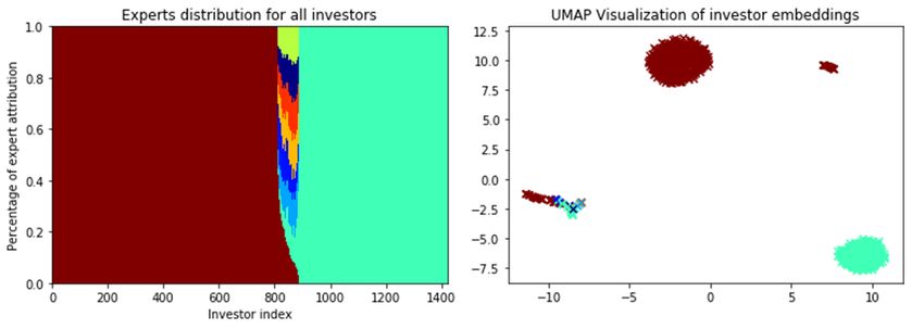
The left-hand plot of Fig. 7 shows the distribution over experts for all the 1422 considered investors. We see three
different patterns appearing : one which used the brown expert only, another one the green expert only and a composite
one. These patterns lead to four clusters on the right-hand plot. In this plot, as previously done in the IBEX experiment,
each point corresponds to an investor, whose color is determined by the expert to which she is mainly attributed, with
colors matching the ones of the left-hand plot. We empirically remark that these clusters all have different activities:
the larger brown cluster is twice more active than the green one, the two smaller clusters having in-between average
activities. The ExNet therefore retrieved distinct behavioural patterns, confirmed by a global rescaled specialization
loss below 0.5, hence negatively correlated experts.
Obtaining finer clusters could be achieved in multiple ways. A higher-level category could be used as gating input:
instead of encoding investors directly, one could encode their sector of activity, in the fashion of the non-universality of
clients experiment. With an encoding of the investors, running an ExNet on the investors of one of the retrieved clusters
only would also lead to a finer clustering of the investors — a two-stage gating process could even directly lead to it,
and will be part of further investigations on the ExNet algorithm. Note however that these maps (and ExNets) are built
from measures of simultaneous distance, hence, do not exploit lead-lag relationships — how ExNets could be adapted
to a temporal setting to retrieve lead-lag relationships will be worthy of future investigations as well.
Figure 7: Distribution over experts of all investors and UMAP visualization of investors embeddings for the ExNet
algorithm on the BNPP CIB Bonds’ RFQ dataset. Each column of the left plot shows the attribution probabilities of a
given investor, where colors represent experts — same colors are used on the right plot.
On a global scale, these plots help us understand how investors relate to each other. Therefore, one can use them to
obtain a better understanding of BNP Paribas CIB business, and how BNP Paribas CIB clients’ behave on a given
market through a thorough analysis of the learnt experts.
12Deep prediction of investor interest: a supervised clustering approach A P REPRINT
5 Conclusion
We introduced a novel algorithm, ExNet, based on the financial intuition that in a given market, investors may act
differently when exposed to the same signals, and cluster around a finite number of investment strategies. This algorithm
is able to perform both prediction, be it regression or classification, and clustering at the same time. The fact that
these operations are trained simultaneously leads to a clustering that most closely serves the prediction task, and a
prediction that is improved by the clustering. Moreover, one can use this clustering a posteriori, independently, to
gain knowledge as to how individual agents behave and interact with each other. To help the clustering process, we
introduced two additional loss terms that penalize the correlation between the inferred investment strategies and the
entropy of the investors’ allocations to experts. Thanks to an experiment with simulated data, we proved the usefulness
of our approach, and we discussed how the ExNet algorithm performs on an open-source dataset of Spanish stock
market data and on data from BNP Paribas CIB. Further research on the subject will include how such architectures
could be extended and staged, and how they could be adapted to retrieve lead-lag relationships in a given market.
On a final note, the ExNet architecture introduced in this article can be applied wherever one expects agents to use a
finite number of decision patterns, e.g. in e-shopping or movie opinion databases [Bennett et al., 2007].
6 Acknowledgements
This work was conducted under the French CIFRE PhD Program, in collaboration between the MICS Laboratory at
CentraleSupélec and BNP Paribas CIB Global Markets. We thank Sarah Lemler, Frédéric Abergel and Julien Dinh for
helpful discussions and feedback on early drafts of this work.
13Deep prediction of investor interest: a supervised clustering approach A P REPRINT
References
K. Baltakys, J. Kanniainen, and F. Emmert-Streib. Multilayer aggregation with statistical validation: Application to
investor networks. Scientific reports, 8(1):8198, 2018.
J. Bennett, S. Lanning, et al. The Netflix Prize. In Proceedings of KDD cup and workshop, volume 2007, page 35. New
York, NY, USA., 2007.
J. Bergstra and Y. Bengio. Random search for hyper-parameter optimization. Journal of Machine Learning Research,
13(Feb):281–305, 2012.
L. Breiman. Random forests. Machine learning, 45(1):5–32, 2001.
D. Challet, R. Chicheportiche, M. Lallouache, and S. Kassibrakis. Statistically validated lead-lag networks and inventory
prediction in the foreign exchange market. Advances in Complex Systems, 21(08):1850019, 2018.
N. V. Chawla, K. W. Bowyer, L. O. Hall, and W. P. Kegelmeyer. Smote: synthetic minority over-sampling technique.
Journal of artificial intelligence research, 16:321–357, 2002.
J. Davis and M. Goadrich. The relationship between Precision-Recall and ROC curves. In Proceedings of the 23rd
international conference on Machine learning, pages 233–240. ACM, 2006.
T. Dozat. Incorporating Nesterov momentum into Adam. 2016.
M. Gutiérrez-Roig, J. Borge-Holthoefer, A. Arenas, and J. Perelló. Mapping individual behavior in financial markets:
synchronization and anticipation. EPJ Data Science, 8(1):10, 2019.
S. Ioffe and C. Szegedy. Batch normalization: Accelerating deep network training by reducing internal covariate shift.
arXiv preprint arXiv:1502.03167, 2015.
R. A. Jacobs, M. I. Jordan, S. J. Nowlan, and G. E. Hinton. Adaptive mixtures of local experts. Neural computation, 3
(1):79–87, 1991.
G. Ke, Q. Meng, T. Finley, T. Wang, W. Chen, W. Ma, Q. Ye, and T.-Y. Liu. LightGBM: A highly efficient gradient
boosting decision tree. In Advances in Neural Information Processing Systems, pages 3146–3154, 2017.
D. P. Kingma and J. Ba. Adam: A method for stochastic optimization. arXiv preprint arXiv:1412.6980, 2014.
T.-Y. Lin, P. Goyal, R. Girshick, K. He, and P. Dollár. Focal loss for dense object detection. In Proceedings of the IEEE
international conference on computer vision, pages 2980–2988, 2017.
Y. Liu and X. Yao. Simultaneous training of negatively correlated neural networks in an ensemble. IEEE Transactions
on Systems, Man, and Cybernetics, Part B (Cybernetics), 29(6):716–725, 1999.
L. McInnes, J. Healy, and J. Melville. Umap: Uniform manifold approximation and projection for dimension reduction.
arXiv preprint arXiv:1802.03426, 2018.
F. Musciotto, L. Marotta, J. Piilo, and R. N. Mantegna. Long-term ecology of investors in a financial market. Palgrave
Communications, 4(1):92, 2018.
V. Nair and G. E. Hinton. Rectified linear units improve restricted boltzmann machines. In Proceedings of the 27th
international conference on machine learning (ICML-10), pages 807–814, 2010.
Y. E. Nesterov. A method for solving the convex programming problem with convergence rate o(1/k 2 ). In Dokl. akad.
nauk Sssr, volume 269, pages 543–547, 1983.
D. L. Padial. Technical Analysis Library using Pandas. https://github.com/bukosabino/ta, 2018.
N. Shazeer, A. Mirhoseini, K. Maziarz, A. Davis, Q. Le, G. Hinton, and J. Dean. Outrageously large neural networks:
The sparsely-gated mixture-of-experts layer. arXiv preprint arXiv:1701.06538, 2017.
J. Sirignano and R. Cont. Universal features of price formation in financial markets: Perspectives from deep learning.
2018.
N. Srivastava, G. Hinton, A. Krizhevsky, I. Sutskever, and R. Salakhutdinov. Dropout: A simple way to prevent neural
networks from overfitting. The Journal of Machine Learning Research, 15(1):1929–1958, 2014.
I. Sutskever, J. Martens, G. Dahl, and G. Hinton. On the importance of initialization and momentum in deep learning.
In International conference on machine learning, pages 1139–1147, 2013.
M. Tumminello, F. Lillo, J. Piilo, and R. N. Mantegna. Identification of clusters of investors from their real trading
activity in a financial market. New Journal of Physics, 14(1):013041, 2012.
S. E. Yuksel, J. N. Wilson, and P. D. Gader. Twenty years of mixture of experts. IEEE transactions on neural networks
and learning systems, 23(8):1177–1193, 2012.
M. R. Zhang, J. Lucas, G. Hinton, and J. Ba. Lookahead optimizer: k steps forward, 1 step back. arXiv preprint
arXiv:1907.08610, 2019.
14You can also read