Analysis of vineyard differential management zones and relation to vine development, grape maturity and quality
←
→
Page content transcription
If your browser does not render page correctly, please read the page content below
Instituto Nacional de Investigación y Tecnología Agraria y Alimentaria (INIA)      Spanish Journal of Agricultural Research 2012 10(2), 326-337
Available online at www.inia.es/sjar                                                                                         ISSN: 1695-971-X
http://dx.doi.org/10.5424/sjar/2012102-370-11                                                                                 eISSN: 2171-9292

     Analysis of vineyard differential management zones and relation
             to vine development, grape maturity and quality
           J. A. Martinez-Casasnovas1*, J. Agelet-Fernandez1, J. Arno2 and M. C. Ramos1
                                      Department of Environment and Soil Science
                                                 1

     2
         Department of Agro-Forestry Engineering. University of Lleida. Av. Rovira Roure 191, 25198 Lleida. Spain

Abstract
   The objective of research was to analyse the potential of Normalized Difference Vegetation Index (NDVI) maps from
satellite images, yield maps and grapevine fertility and load variables to delineate zones with different wine grape prop-
erties for selective harvesting. Two vineyard blocks located in NE Spain (Cabernet Sauvignon and Syrah) were analysed.
The NDVI was computed from a Quickbird-2 multi-spectral image at veraison (July 2005). Yield data was acquired by
means of a yield monitor during September 2005. Other variables, such as the number of buds, number of shoots, number
of wine grape clusters and weight of 100 berries were sampled in a 10 rows × 5 vines pattern and used as input variables,
in combination with the NDVI, to define the clusters as alternative to yield maps. Two days prior to the harvesting, grape
samples were taken. The analysed variables were probable alcoholic degree, pH of the juice, total acidity, total phenolics,
colour, anthocyanins and tannins. The input variables, alone or in combination, were clustered (2 and 3 Clusters) by using
the ISODATA algorithm, and an analysis of variance and a multiple rang test were performed. The results show that the
zones derived from the NDVI maps are more effective to differentiate grape maturity and quality variables than the zones
derived from the yield maps. The inclusion of other grapevine fertility and load variables did not improve the results.
   Additional key words: cluster analysis; differential management zones; NDVI; precision viticulture; selective
harvesting; yield maps.

Resumen
Análisis de zonas de manejo diferencial en viñedo y relación con el desarrollo de la viña, madurez y calidad de la uva
   El objetivo de la investigación fue analizar el potencial de mapas del índice de vegetación de la diferencia normaliza-
da (NDVI) a partir de imágenes de satélite, mapas de cosecha y variables de fertilidad y carga de las cepas para delinear
zonas de manejo con diferentes propiedades de madurez y calidad de la uva. Se estudiaron dos parcelas localizadas en el
NE de España (Cabernet Sauvignon y Syrah). El NDVI fue derivado de una imagen multiespectral Quickbird-2 adquiri-
da en el envero (julio 2005). Los datos de cosecha fueron obtenidos por medio de un monitor de rendimiento en septiem-
bre de 2005. Otras variables, tales como el número de yemas, número de sarmientos, número de racimos y peso de
100 bayas fueron muestreados en un marco de 10 filas × 5 cepas. Estas variables fueron usadas, en combinación con el NDVI,
para definir los aglomerados (clusters) como alternativa a los derivados de los mapas de cosecha. Dos días antes de la
vendimia se muestreó la uva. Las propiedades analizadas fueron el grado alcohólico probable, el pH del mosto, la acidez
total, los polifenoles totales, el color, los antocianos y los taninos. Las variables de entrada, solas o en combinación,
fueron aglomeradas (2 y 3 aglomerados) por medio del algoritmo ISODATA, llevando a cabo después un análisis de
varianza y de rangos múltiples. Los resultados muestran que las zonas derivadas de los mapas de NDVI son más efectivos
para diferenciar uvas con diferentes propiedades de madurez y calidad que no las zonas derivadas de los mapas de cose-
cha. La inclusión de otras variables de fertilidad y carga de las cepas no mejoró los resultados.
   Palabras clave adicionales: análisis de aglomerados; mapas de cosecha; NDVI; vendimia selectiva; viticultura de
precisión; zonas de manejo diferencial.

*Corresponding author: j.martinez@macs.udl.es
Received: 29-07-11. Accepted: 29-02-12

Abbreviations used: ANOVA (analysis of variance); CV (coefficient of variation); ISODATA (iterative self-organizing data
analysis); NDVI (normalized difference vegetation index); NIR (near infrared); PA (precision agriculture); PV (precision viticulture);
SD (standard deviation); VESPER (variogram estimation and spatial prediction plus error); WG (number of wine grape clusters);
100B (weight of 100 berries).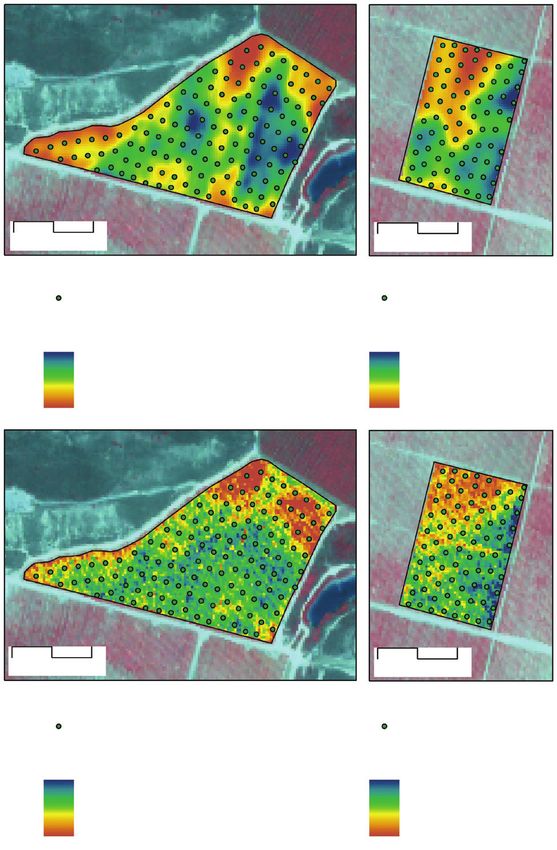
Vineyard management zones and relation to vine development, grape maturity and quality 327
Introduction amelioration prior to vineyard establishment, being
based on the results of few samples because of the high
Vineyard variability is a known phenomenon of cost of soil analysis. This has been partially overcome,
which viticulturists are generally aware, understanding according to some experiments, by the use of the
that vine performance varies within their vineyards apparent soil electrical conductivity (EC a) measure-
(Bramley & Hamilton, 2004; Bramley et al., 2011). ment, as parameter that shows good correlations to
The development of the spatial information technolo- reference soil properties (Corwin & Lesch, 2005;
gies tools in the last decades and the advent of grape Samouëlian et al., 2005; Bramley et al., 2011;
yield sensors and monitors has allowed obtaining in- Rodriguez-Perez et al., 2011). Nevertheless, although
formation on vine performance as well as soil variabil- topographical conditions and soil variation have been
ity across the vineyard fields (Proffitt & Malcolm, recognized to be influencing grape growth and the
2005; Proffitt et al., 2006). Then, the opportunity of sensory and chemical characteristics of the wines de-
the analysis of vineyard spatial variability is important rived from them (Bramley et al., 2011), we can still
from the perspective of Precision Viticulture (PV), observe a relative lack of emphasis placed on this area
since it allows the identification of zones of different by viticulturists, and soil information is not usually
productive potential within the parcel and an evaluation used for management zone delineation.
of the opportunity for their differential management Vine vegetation development has been also recog-
(Bramley, 2005; Arno et al., 2009). nised as a factor related to wine grape quality (Hall
The system of differential management has been et al., 2002; Cortell et al., 2005). It can be determined
referred to as zonal vineyard management (Bramley, by field measures on selected vines (e.g. trunk cross-
2005). Several examples of this approach improving sectional area, average shoot length, and leaf chloro-
the uniformity of fruits delivered to the winery have phyll (Cortell et al., 2005), or by means of optical re-
been already demonstrated. For example, experiences mote sensing (Rouse et al., 1973; Myneni et al., 1995;
to improve labour at pruning, to forecast yield or to Lamb et al., 2004). To measure the continuous spatial
apply cultural practices differentially, as for example variability of vine vigour, optical remote sensing pro-
irrigation water, with distinct amounts in different vides a synoptic view of grapevine photosynthetically-
management zones along the growing season, have active biomass over entire vineyards and appear to be
been reported (Proffitt & Pearse, 2004; Martinez- a management tool of enormous potential with red
Casasnovas & Bordes, 2005; Proffit & Malcolm, 2005; grape varieties, especially if the canopy architecture
Martinez-Casasnovas et al., 2009). Nevertheless, the can be linked to production of phenolics and colour in
major number of experiences has been addressed to selec- ripe grapes (Lamb et al., 2004). Other authors have
tive harvesting, since the attempt to diminish within-field considered the possibility of substituting the informa-
yield variability is difficult because it is mainly related tion obtained from remote sensing (satellite or aerial
to soil property differences, which are difficult to change images) by optical proximal sensors computing vegeta-
(Proffitt & Malcolm, 2005). Fruit quality has also shown tion indexes and ultrasonic sensors to identify areas
to be variable. Its patterns of spatial variation tend to presenting critical vegetation conditions (Mazzetto
follow those for yield, although not necessarily in the et al., 2010), or have experimented with reflection
same rank order (Bramley & Hamilton 2004, 2007). radiometers to characterize spectral features of vine-
Because of that, selective harvesting only based on intra- yards (da Silva & Ducati, 2009).
field yield variability may not correspond with wine The most used indices from remote sensing data in
grapes of significant different qualities (Hall et al., 2003). PV have been the PCD (plant cell density) (Hall et al.,
This makes interesting to analyse relationships between 2002; Proffitt & Malcolm, 2005), calculated as the ratio
wine grape quality properties and other spatial variables between the near infrared to red reflectance; the PRV
that could influence grape yield and quality, helping in (photosynthetic vigour ratio), calculated as the ratio
the delineation of management zones. between green to red reflectance; and the NDVI (nor-
In this respect, some studies point out the importance malized difference vegetation index), calculated by
to know in detail the spatial variability of chemical and the combination of near infrared and red reflectances
physical soil properties for the successful adoption of (NIR-R/NIR + R) (Rouse et al., 1973). In some cases,
PV (Bramley et al., 2011). Most of the effort in soil these vigour indices have been used in combination
analysis goes into assessment of fertilisation and soil with other vegetative vine variables to predict the spa-328 J. A. Martinez-Casasnovas et al. / Span J Agric Res (2012) 10(2), 326-337
tial variability of yield (Martinez-Casasnovas & Bor- mation, sprinkle irrigation, planted in 1986) and Syrah
des, 2005; Taylor et al., 2010), in combination with (2.35 ha, Vertical Shoot Position formation, drip partial
yield to help in the delineation of uniform management root drying irrigation, planted in 2002). The viticultur-
zones to improve irrigation (Proffitt & Malcolm, 2005; ist maintains an herbaceous ground cover between the
Martinez-Casasnovas et al., 2009), or to delineate rows of vines. Soils in these fields are classified as
management zones for selective harvesting (Johnson Fluventic Haploxerepts, Calcic Haploxerepts and Ty
et al., 2001; Bramley et al., 2011). However, the use pic Haploxerepts (Soil Survey Staff, 2006). The Typic
of these indices in PV is becoming to have some criti- Haploxerepts may present a paralithic contact within
cisms because, as well as it happens with yield spatial the first 50 cm, which could represent a limitation for
variability and grape quality, the spatial variation pat- vine development. Both vineyards are on gentle slopes
tern of these indices is not necessarily the same as the (2-7%) and south faced terrain.
variation of grape quality (Bramley, 2005). Other vine
variables determining the vine crop load should be
taken into account, together with vegetation vigour Data acquisition and analysis
indices, to delineate consistent management zones for
selective harvesting (Santesteban & Royo, 2006; San- The research was carried out with data collected
testeban et al., 2008). In this respect, these authors during the 2005 campaign. First, a Quickbird-2 multi-
propose to complement zoning based on NDVI with spectral image was acquired on 13-07-2005, date
vine load variables such as bunch number per vine or within the range of ±2 weeks the moment of veraison,
berry weight per bunch, since vine load determines which has been referred to be the optimal time for
grape quality for vines with similar vegetation develop- image acquisition in PV applications (Lamb et al.,
ment and hydric stress. 2004). The spatial resolution of the multi-spectral
At the moment, vegetation indexes from detailed image was 2.8 m. The image was corrected for atmos-
remote sensing data (satellite or aerial images) consti- pheric scattering by applying the COST model pro-
tute the main source of data that is used in PV for de- posed by Chavez (1996). Digital values were con-
lineation of differential management zones as alterna- verted to reflectance according to the radiance
tive to yield maps. On the other hand, and in the conversion of Quickbird-2 data technical note (Krause,
absence of detailed soil data, other vine variables (e.g. 2003). After this process, the images were projected to
determining the vine crop load) should be taken into the European Datum 1950 and the UTM 31n coordinate
account to improve management zone delineation. In system. The projected images were then ortho-rectified
this respect, the present research shows a case study in based on: a) a set of ground control points collected from
which the objective was to analyse the potential of a 0.5-m resolution ortho-photo, and b) a 5-m resolution
NDVI (derived from high resolution satellite images), digital elevation model, both produced by the Carto-
alone or together with other wine grape fertility and graphic Institute of Catalonia. The NDVI was computed
load variables, and yield maps acquired by means of according to Eq. 1 (Rouse et al., 1973) (Fig. 1).
yield monitors, in order to establish zones with differ- ϕ NIR − ϕ RED
ent grapes maturity and quality variables. NDVI = [1]
ϕ NIR + ϕ RED
where jNIR and jRED are the spectral reflectance meas-
Material and methods urements acquired in the near-infrared (760-900 nm)
and red (630-690 nm), respectively for the case of
Study area Quickbird-2. These spectral reflectances are themselves
ratios of the incoming radiation that is reflected in each
The case study was conducted in two vineyard fields spectral band individually, hence they take on values
located in Raimat (Costers del Segre Denomination of between 0.0 and 1.0. By design, the NDVI itself thus
Origin, Lleida, NE Spain; 291910 E, 4615070N, 270 m, varies between –1.0 and +1.0. NDVI values in the
UTM 31 T). This is a semi-arid area with continental 2.8 pixel size of the Quickbird-2 image were influenced
Mediterranean climate and a total annual precipitation by the herbaceous cover between the vine rows main-
between 300-400 mm. The fields are planted in a 3 × 2 m tained by the viticulturist. This, however, did not sig-
pattern with Cabernet Sauvignon (5 ha, T system for- nificantly influence the use of this index in NDVIVineyard management zones and relation to vine development, grape maturity and quality 329
(a) (b) ing records for which the Normalized yield was greater
or less than ± 3 standard deviations from the mean. The
resulting yield data were used to interpolate 3 m grid by
local block kriging (10 m × 10 m blocks) using VESPER
(Minasny et al., 2005) (Fig. 1).
Along the vegetative cycle of the year, and in a
10 rows × 5 vine pattern (sample density of 30 sam-
ples ha –1, see location of sampling points in Fig. 1),
0 25 50
m
100 0 25 50
m
100
the following grapevine fertility and load variables
Cabernet Sauvignon block Syrah block were measured (per lineal meter): number of buds,
Sampling points Sampling points number of shoots, number of wine grape clusters. The
YIELD 2005 YIELD 2005 sample density was similar to that proposed by Bram-
Value Value
High : 11.6 High : 11.8 ley (2005), who suggested that it enables production
of robust maps of vine variation. The sample vines were
Low : 1.5 Low : 1.9
georeferenced using a Trimble Geo-explorer XT, which
has sub-metric precision after differential corrections
in post-processing. Two days prior to the harvesting,
and in the same sampling pattern, samples of wine
grape clusters were collected to determine the weight
of 100 berries. The collected grapes were kept in a
portable cool box till they reached the laboratory where
they were processed. The analysed variables were, for
m m grape maturity: pH of the juice, total acidity (expressed
0 25 50 100 0 25 50 100
as g H2SO4 L–1) and probable alcoholic degree of the
Cabernet Sauvignon block Syrah block
Sampling points Sampling points
juice (º Baumé); and for grape quality variables: total
NDVI NDVI grape phenolics (expressed as absorbance at 420 nm),
Value
High : 0.65
Value
High : 0.55
colour (expressed as sum of the absorbance at 420 nm,
520 nm and 620 nm), anthocyanins (mg g–1) and tannins
Low : 0.23 Low : 0.21
(mg g–1). For the preparation of the samples the meth-
Figure 1. Yield and NDVI maps of the Cabernet Sauvignon (a) ods proposed in Iland et al. (2004) were applied.
and Syrah (b) blocks for the 2005 vintage. The samples of the grapevine fertility and load
variables were interpolated to the 3 m grid previously
zoning since, according to field observations, the established by global kriging using VESPER (Minasny
change of vigour of the herbaceous vegetation was et al., 2005). Several semivariogram models were ap-
coincident in the space with the changes of vine veg- plied (spherical, exponential and lineal with threshold).
etation vigour. The model that was selected for each variable was the
Yield data was acquired by means of a Canlink 3000 one minimizing the Sum of Squared Error, the Akaike
Farmscan monitor (Bentley, WA, Australia) during Sep- Index Criterion and the Root Mean Square Error.
tember 2005. The system basically consists of a set of NDVI, grapevine fertility/load variables and yield
load cells installed on the grape discharge arm of the maps were clustered using the ISODATA algorithm
grape harvester. By measuring grape weight and other implemented in Image Analyst for ArcGIS 9.3. The
required variables, such as the harvester speed and posi- ISODATA is a k-means algorithm that uses minimum
tion of the harvester, the yield monitor calculates the Euclidean distance to assign a cluster to each candidate
production in Mg ha–1 at different locations in the parcel pixel in an iterative process (Jensen, 1996), removing
(Arno et al., 2005, 2009). The monitor was programmed redundant clusters or clusters to which not enough sam-
to weight the grapes at 3 second intervals. From these ples are assigned. In the present case study the target
data, a yield map was produced following the protocol clusters (zones) were two or three, according to previous
of Bramley & Williams (2001). Data refinement involved experiences of definition of management zones in dif-
normalising the data (μ = 0, s = 1) after removal of data ferent study areas (Bramley & Hamilton, 2004; Arno
records with zero yield or GPS errors, and then remov- et al., 2005; Proffitt & Malcolm, 2005). The clusters330 J. A. Martinez-Casasnovas et al. / Span J Agric Res (2012) 10(2), 326-337
were created according to the following combination of variable with the highest coefficients of variation (30.1
input variables: a) NDVI, b) Yield, c) NDVI, number of and 32.2%, respectively), which indicate a potential
wine grape clusters and weight of 100 berries, d) NDVI, for PV applications as zonal management or selective
number of buds, number of shoots, number of wine grape harvesting (Bramley & Hamilton, 2004). Grapevine
clusters and weight of 100 berries. fertility and load variables, such as the number of buds,
The georeferenced vines, where grape samples were number of shoots, number of wine grape clusters and
taken, were converted to a point shapefile layer using the weight of 100 berries also show intra-field variation
ArcGIS.9.3. Then, the previously identified zones were but in a different rank order than yield. It is closer to
assigned to the sample points according to their spatial the coefficients of variation of the NDVI than to the
location. All the data relative to sample points were yield.
held in a table that was statistically analysed using the Regarding wine grape maturity and quality char-
SAS software. An ANOVA test and a Duncan multiple acteristics, colour, anthocyanins, tannins, total acid-
rang analysis were applied to the classified samples to ity and total phenolics are the properties with higher
analyse the separation of means and determine sig- variability in both vineyard blocks, with maximum
nificant differences between them. For each vineyard CV values of 24.5% and 28.1% in the case of juice
block, the results were summarized according to the colour. Probable alcoholic degree and juice pH are
number of variables differentiated in each group of the most homogeneous variables, with CV between
clusters. From these data, the global number of pre- 3.9% and 9.9%.
dicted variables was compared to the potential number
of cases and a χ2 test was performed to determine sig-
nificant differences between blocks. Relationships between NDVI and yield
variation zones and vineyard performance
Results Using the maps of the NDVI, yield and grapevine
fertility and load variables, four types of clusters were
Summarized statistics of the sampled created according to the combination of input variables
variables described in the “Data acquisition and analysis” sec-
tion. Here the results of the multiple rang analysis
Table 1 presents the basic statistics of the sampled between NDVI or yield zones (defined by means of
variables in the case study vineyard blocks. Yield is the clustering) are presented. Tables 2 and 3 present these
Table 1. Basic statistics of the sampled variables in the vineyard blocks of the case study:
Cabernet Sauvignon and Syrah
Cabernet Sauvignon Syrah
Variable (n = 128) (n = 77)
mean ± SD CV% mean ± SD CV%
NDVI 0.5 ± 0.07 13.1 0.4 ± 0.07 19.0
Yield (Mg ha–1) 6.9 ± 2.1 30.1 6.9 ± 2.2 32.2
Buds (No. m–1) 7.9 ± 1.0 12.6 9.6 ± 0.6 6.6
Canes (No. m–1) 7.6 ± 0.9 11.8 11.6 ± 0.5 4.3
Grapevine clusters (No. m–1) 11.0 ± 1.6 14.5 11.3 ± 2.2 19.5
Weight of 100 berries (g) 138.6 ± 19.6 14.1 177.9 ± 23.4 13.2
° Baumé 14.3 ± 0.9 6.8 14.9 ± 1.5 9.9
pH 4.2 ± 0.1 4.0 3.8 ± 0.1 3.9
Total acidity (g H2SO4 L–1) 2.9 ± 0.5 15.3 3.6 ± 0.4 11.6
Total phenolics (au) 12.0 ± 1.9 15.7 12.8 ± 1.9 14.7
Colour (au) 4.2 ± 1.0 24.5 5.2 ± 1.4 28.1
Anthocyanins (mg g–1) 0.66 ± 0.17 25.7 0.81 ± 0.05 26.2
Tannins (mg g–1) 0.18 ± 0.04 22.2 0.23 ± 0.05 21.7
n: number of samples. SD: standard deviation. au: absorbance units.Vineyard management zones and relation to vine development, grape maturity and quality 331
Table 2. Multiple rang analysis in zones defined by the NDVI: Cabernet Sauvignon block (CS) and Syrah block (Sy)
Wine
Total 100-berries
Yield Total acidity Anthocyanins Tannins Colour Buds Shoots grape
Clusters NDVI ºB pH phenolics weight
(Mg ha–1) (g H2SO4 L–1) (mg g–1) (mg g–1) (au) m-1 m-1 clusters
(au) (g)
m-1
CS-2C Cluster 1 0.44 5.65 14.55 3.84 2.72 12.93 0.73 0.20 4.63 128.18 7.83 7.71 10.84
n = 48 A A B B A B B B B A A A A
Cluster 2 0.54 7.79 14.11 3.72 3.13 11.44 0.62 0.17 3.92 144.91 7.92 7.56 11.14
n = 80 B B A A B A A A A B A A A
CS-3C Cluster 1 0.41 5.41 14.04 3.87 2.67 13.41 0.76 0.21 4.87 123.81 7.62 7.56 10.48
n = 22 A A A B A C B C B A A A A
Cluster 2 0.50 6.36 14.77 3.77 2.83 12.28 0.69 0.19 4.39 135.45 7.93 7.80 11.21
n = 42 B A B A A B B B B B A A A
Cluster 3 0.55 7.94 14.03 3.72 3.17 11.33 0.60 0.16 3.81 145.82 7.97 7.52 11.08
n = 64 C B A A B A A A A C A A A
Sy-2C Cluster 1 0.32 5.56 15.90 3.87 3.44 14.01 0.89 0.25 5.75 165.95 9.90 11.90 10.02
n = 40 A A B B A B B B B A B B A
Cluster 2 0.43 8.29 14.00 3.74 3.70 11.58 0.71 0.19 4.51 190.91 9.27 11.35 12.72
n = 37 B B A A B A A A A B A A B
Sy-3C Cluster 1 0.30 4.98 16.34 3.88 3.42 14.41 0.92 0.26 5.95 159.74 9.99 12.11 9.64
n = 27 A A C B A C B C C A B B A
Cluster 2 0.39 7.20 14.65 3.78 3.59 12.74 0.82 0.22 5.23 184.62 9.49 11.35 11.76
n = 29 B B B A AB B B B B B A A B
Cluster 3 0.45 8.85 13.71 3.75 3.70 10.96 0.63 0.17 4.04 192.14 9.23 11.41 12.86
n = 21 C C A A B A A A A B A A C
C: Clusters; n = number of samples. au: absorbance units. The data in the columns correspond to the mean of the samples in each clus-
ter. The letter indicates statistical differences between clusters with a p–value < 0.05.
results for the Cabernet Sauvignon and Syrah blocks number of wine grape clusters and weight of 100 ber-
(NDVI and yield based clusters, respectively). In these ries, indicative of grapevine fertility and load, only the
tables, NDVI or yield zones as referred to as clusters. weight of 100 berries showed a good relationship either
Then, in the case of two clusters (zones), cluster 1 cor- in two zones or three zones in the Cabernet Sauvignon
responds with the low NDVI or yield zone values and block, but only in two zones the Syrah block. The
cluster 2 the high NDVI or yield zone values. In the case number of wine grape clusters in the Syrah block was
of three clusters, cluster 2 corresponds with the medium another variable showing a direct relationship with
NDVI or yield zone values while cluster 3 with the high NDVI (2 or 3 zones) and yield (only 2 zones).
NDVI or yield zone values. The results for the clusters The results of multiple rang analysis in wine grape
created with the NDVI, number of wine grape clusters maturity variables with respect NDVI and yield in both
and weight of 100 berries; and with the NDVI, number blocks (Tables 2 and 3), reveal a better performance of
of buds, number of shoots, number of wine grape clusters zones derived from the NDVI maps than from the yield
and weight of 100 berries, were summarized in Table 4. data. The probable alcoholic degree in the Cabernet
First, a direct relationship between NDVI zones and Sauvignon block, that presents a similar CV as the Syrah
yield is observed in both vineyard blocks, with signifi- block (< 10%), is the only variable that does not present
cant separation of yield means in NDVI zones and vice- a clear differentiation either in the NDVI or yield zones.
versa when considering the analysis of two clusters (Fig. Nevertheless, in the Cabernet Sauvignon block there is
2). In the case of three clusters, only the Syrah block, a trend towards an increase of the probable alcoholic
with higher intra-field variability of vegetation develop- degree of the wine grapes with lower yields. In the case
ment, presented statistical significant differences. of NDVI zones this trend is not confirmed, probably due
In the case of the relationship between NDVI or to the effect of the irrigation system (sprinkle irrigation)
yield with the number of buds, number of shoots, in the development of spontaneous vegetation (weeds)332 J. A. Martinez-Casasnovas et al. / Span J Agric Res (2012) 10(2), 326-337
Table 3. Multiple rang analysis in zones defined by the yield: Cabernet Sauvignon (CS) and Syrah blocks (Sy)
Wine
Total 100-berries
Yield Total acidity Anthocyanins Tannins Colour Buds Shoots grape
Clusters NDVI ºB pH phenolics weight
(Mg ha–1) (g H2SO4 L–1) (mg g–1) (mg g–1) (au) m-1 m-1 clusters
(au) (g)
m-1
CS-2C Cluster 1 5.00 0.47 14.50 3.79 2.82 12.66 0.71 0.19 4.55 130.87 7.85 7.73 11.07
n = 55 A A B A A B B B B A A A A
Cluster 2 8.48 0.53 14.10 3.74 3.09 11.50 0.61 0.17 3.91 144.49 7.91 7.53 10.99
n = 73 B B A A B A A A A B A A B
CS-3C Cluster 1 4.01 0.44 14.51 3.85 2.66 13.22 0.74 0.20 4.75 126.88 7.56 7.63 10.38
n = 27 A A B B A C C C C A A A A
Cluster 2 6.75 0.52 14.37 3.74 3.03 11.97 0.66 0.18 4.23 137.72 7.89 7.51 11.07
n = 62 B B B A B B B B B B AB A AB
Cluster 3 9.24 0.54 13.96 3.75 3.10 11.20 0.58 0.16 3.72 148.23 8.10 7.78 11.39
n = 39 C B A A B A A A A C B A B
Sy-2C Cluster 1 4.91 0.33 15.76 3.85 3.53 13.96 0.89 0.25 5.75 165.48 9.73 11.87 10.03
n = 37 A A B B A B B B B A A B A
Cluster 2 8.69 0.41 14.27 3.76 3.59 11.80 0.72 0.20 4.61 189.47 9.47 11.42 12.51
n = 40 B B A A A A A A A B A A B
Sy-3C Cluster 1 4.42 0.31 15.99 3.87 3.52 14.32 0.90 0.25 5.80 158.35 9.86 12.02 9.91
n = 28 A A B B A C B B B A B B A
Cluster 2 7.11 0.38 14.70 3.79 3.63 12.46 0.78 0.22 5.00 187.61 9.40 11.40 11.73
n = 23 B B A AB A B AB A A B A A B
Cluster 3 9.30 0.43 14.16 3.75 3.54 11.58 0.72 0.20 4.61 189.65 9.48 11.42 12.47
n = 26 C C A A A A A A A B A A B
C: Clusters; n = number of samples. au: absorbance units. The data in the columns correspond to the mean of the samples in each
cluster. The letter indicates statistical differences between clusters with a p–value < 0.05.
Table 4. Frequency data of the grapevine fertility/load and wine grape maturity/quality variables with differentiation in the
multiple rang analysis test per type of zone definition: Cabernet Sauvignon block / Syrah block
Grapevine fertility / load Wine grape maturity Wine grape quality
Zone variables1 (4 variables) (3 variables) (4 variables) Total Accuracy (%)
2 clusters 3 clusters 2 clusters 3 clusters 2 clusters 3 clusters
NDVI 1/2 0/1 3/3 0/1 4/4 2/3 10 / 14 45.5 / 63.6
Yield 1/2 1/0 2/2 1/0 4/4 4/0 13 / 80 59.1 / 36.4
NDVI, WG clusters, 100B 0/2 0/2 3/2 0/0 4/4 3/1 10 / 11 45.5 / 50.0
NDVI, Buds, Shoots, WG clusters, 100B 0/2 0/2 3/3 0/0 4/4 1/3 8 / 14 36.4 / 63.6
Total 2/8 1/5 11 / 10 1/1 16 / 16 10 / 7 41 / 47
Global accuracy (%) 46.6 / 53.0
1
WG: number of wine grape clusters; 100B: weight of 100 berries.
between the vine rows that, to some extent, influences presents the lowest CV among the tested variables
the NDVI value of vines. In the Syrah block, with drip (Table 1), it shows significant differentiation in both
irrigation and less development of spontaneous vegeta- vineyard blocks, in particular in the 2-NDVI zones (Table
tion between the rows, there are significant differences 2). In the case of 3-NDVI or 3-yield zones, the moderate/
of probable alcoholic degree in either the NDVI or yield medium zone shows an ambiguous behaviour, being
zones, except in the case of 3-yield zones, in which there either grouped with the low or the high NDVI or yield
is not a clear differentiation between the moderate and zones. However, there is a trend of the pH values towards
high yield zones. In relation to juice pH, although it an increase as the NDVI values or yield decrease.Vineyard management zones and relation to vine development, grape maturity and quality 333
(a) (b)
m m m m
0 25 50 100 0 25 50 100 0 25 50 100 0 25 50 100
Cabernet Sauvignon block Cabernet Sauvignon block Syrah block Syrah block
Sampling points Sampling points Sampling points Sampling points
YIELD Zones NDVI Zones YIELD Zones NDVI Zones
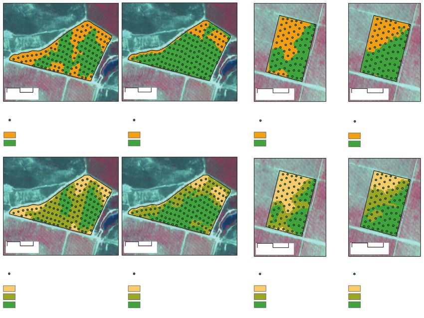
Zone 1 (Low yield: 5.0 Mg ha )
–1
Zone 1 (Low NDVI: 0.44) Zone 1 (Low yield: 4.91 Mg ha–1) Zone 1 (Low NDVI: 0.32)
Zone 2 (High yield: 8.48 Mg ha–1) Zone 2 (High NDVI: 0.54) Zone 2 (High yield: 8.69 Mg ha–1) Zone 2 (High NDVI: 0.43)
m m m m
0 25 50 100 0 25 50 100 0 25 50 100 0 25 50 100
Cabernet Sauvignon block Cabernet Sauvignon block Syrah block Syrah block
Sampling points Sampling points Sampling points Sampling points
YIELD Zones NDVI Zones YIELD Zones NDVI Zones
Zone 1 (Low yield: 4.01 Mg ha )
–1
Zone 1 (Low NDVI: 0.41) Zone 1 (Low yield: 4.42 Mg ha–1) Zone 1 (Low NDVI: 0.30)
Zone 2 (Medium yield: 6.75 Mg ha–1) Zone 2 (High NDVI: 0.50) Zone 2 (Medium yield: 7.11 Mg ha–1) Zone 2 (High NDVI: 0.39)
Zone 3 (High yield: 9.24 Mg ha–1) Zone 2 (High NDVI: 0.55) Zone 3 (High yield: 9.30 Mg ha–1) Zone 2 (High NDVI: 0.45)
Figure 2. Yield and NDVI zones created with the algorithm ISODATA for the Cabernet Sauvignon block (a) and the Syrah block
(b). Upper part: two Yield or NDVI zones; lower part: three Yield or NDVI zones. See statistical data in Tables 2 and 3. The numbers
between brackets correspond to the average values in each zone.
Total acidity, although it shows a positive trend with are inverse, which indicates that low vigour or low
respect the increase of NDVI and yield, it presents yield zones are the ones presenting the highest contents
variety differences. This property shows clear differ- of phenolics and the highest values of absorbance units
entiation (either in 2-zones or 3-zones) in the NDVI for colour, anthocyanins and tannins in the grape juice.
clusters in the Cabernet Sauvignon block but not in the In the case of juice colour, however, the differentiation
Syrah block. In this last block total acidity is differen- is not as clear as in the phenolics. For both varieties,
tiated in the two extreme NDVI zones, with the medi- the differentiation of colour performs better in 2-zones
um-NDVI zone being ambiguous. In summary, NDVI than in 3-zones, being the moderate/medium NDVI or
performs better than yield as variable to establish zones yield zone always ambiguous.
with respect total acidity in both blocks since yield
zones only differentiated juice acidity in 2-zones in the
Cabernet Sauvignon block but not in the Syrah. Frequency analysis and best zone definition
Grape quality variables (total phenolics, colour, criteria
anthocyanins and tannins) are the properties that
present the best performance in the defined zones from Which variable or group of input variables for clus-
NDVI or yield clusters. In all cases the relationships ter (zone) definition is the optimal to differentiate zones334 J. A. Martinez-Casasnovas et al. / Span J Agric Res (2012) 10(2), 326-337 for grapevine fertility/load and grape maturity/quality with respect the potential positive cases, indicates that variables? To answer this question a frequency analy- the null hypothesis (the observed frequency distribution sis of the number of these variables that presented is similar to the potential distribution) can be rejected significant differences in the multiple rang analysis for in the case of the Cabernet Sauvignon field with a either 2-zones or 3-zones, and per grapevine variety, p < 0.05 (χ2 = 12.83 with respect χ2p = 0.05 = 12.59), but was done. The results are summarized in Table 4 for not in the case of the Syrah block. This indicates a the Cabernet Sauvignon and the Syrah blocks. general better performance of the grapevine and wine If compared with the potential number of positive grape parameter differentiation in the Syrah block with cases in which the analysed grapevine and wine grape respect the Cabernet Sauvignon block. variables could have been differentiated in one block As mentioned above, the differentiation of the ana- for all types of zone definition (88 positive cases in lysed variables in 3-zones produced poorer results than total), the global accuracy of the differentiation of those in 2-zones. Wine grape quality variables were the ones variables analysed is moderate: 46.6-53.4% in the Ca- that obtained moderate results: 43.8-62.5% of differ- bernet Sauvignon and Syrah blocks respectively. The entiation respectively in the Syrah and Cabernet Sau- results significantly improve if the accuracy is meas- vignon blocks. Other variables yielded accuracies be- ured per number of zones defined: 65.9-77.3% in the tween 6.3 to 31.3%, which confirms the worse case of differentiation in 2-zones against 29.5-30.0% performance of differentiating 3-zones instead of in 3-zones (for Cabernet Sauvignon and Syrah blocks 2-zones for differential management. respectively). Differentiation by yield clusters performed better in the Cabernet Sauvignon block (59.1%), but in the Syrah Discussion block differentiation in NDVI clusters was better (63.6% of the cases). Another relevant result was the The present results in two vineyard blocks of the fact that the use of variables for cluster definition such north-east Spain confirm some previous knowledge in as the number of buds, number of shoots, number of PV that has been experienced in other world viticulture wine grape clusters or weight of 100 berries, did not regions. The values of the basic statistics of the sam- improve the results obtained either with the clustering pled variables are within the range of variability also of NDVI or yield alone. These results do not corrobo- found by Bramley (2005) in Cabernet varieties in Aus- rate the suggestions pointed out by Martinez-Casasno- tralia, who observed more homogeneity in properties vas & Bordes (2005) or Santesteban et al. (2008), who as probable alcoholic degree or pH than acidity, colour proposed that the mapping of crop load (e.g. number or phenolics content. These results point out to a poor of bunches per vine and number of berries per bunch), correspondence between yield or NDVI zones and together with NDVI maps, could help or improve the variables as the probable alcoholic degree or pH. How- delineation of management zones corresponding with ever, the NDVI coefficient of variation (13.1-19%) is more differentiated grape qualities. of the same rank order than total acidity, colour or A deeper analysis of the frequency data per group of phenolics, which could result in a good correspondence grapevine and wine grape variables indicates that, in the of those variables with the NDVI or the NDVI to- case of 2-zones, the wine grape maturity and quality gether with load variables derived clusters. Nonethe- were much better differentiated than grapevine fertility less, there are controversial results by other researchers and load variables. This occurred in both vineyard who found poor relations of grape wine maturity and blocks, with better results in the Syrah block due to the quality variables with either NDVI or yield, e.g. moderate performance of the grapevine fertility and load Acevedo-Opazo et al. (2008) in southern France or variables (50.0% of the cases with respect 12.5% in the Santesteban et al. (2008) in Navarra (Spain), who state Cabernet Sauvignon block). Per number of zones de- that the NDVI has a good correlation with the vegeta- fined, and in the case of 2-zones, NDVI is the variable tive development of vines but wine grape quality is that performed better: 72.7-81.8% of the grapevine and affected by other agronomic factors such as soil prop- wine grape variables were differentiated respectively in erties, water availability or climate characteristics. the Cabernet Sauvignon and Syrah blocks. Regarding the relationship between vigour indices, Finally, regarding the analysis in 2-zones, the χ2 test such as NDVI, and yield, there was not ambiguity in carried out to compare the performance of the blocks the relation between NDVI zones and yield or yield
Vineyard management zones and relation to vine development, grape maturity and quality               335

zones and NDVI, as it was the cases reported by John-         wine quality. Anthocyanins and tannins differentiated
son et al. (2001) or Bramley (2005). However, ambigu-         in both blocks when considering 2 zones but performed
ity in the medium/moderate-vigour or yield zone has           different in 3 zones. In this case (3 zones), anthocyanins
been observed with some grapevine fertility and load          and tannins presented significant differences in the 3
and/or wine grape quality variables such as the prob-         zones when defined on the basis of yield for the Caber-
able alcoholic degree, pH, total acidity or colour. The       net Sauvignon block, but not in the Syrah block. Tan-
results also reveal that differentiation of those variables   nins, however, presented significant differences in 3
in 2-zones is better than in 3-zones, with boundaries of      zones for NDVI-clusters in both blocks.
medium/moderate-vigour or yield zone either needing              Delineation of management zones has been mainly
adjustment (or the entire zone be incorporated into the       based on yield maps produced from data acquired by
remaining zones). According to PV experiences in              means of yield monitors on harvester machines or from
wineries of NE Spain, the differentiation in two vigour       remote sensing vigour indices. However, due to the
or yield zones is the option that is preferred because of     controversial results of the performance of wine grape
a) the occasional ambiguity to classify the medium/           maturity and or quality with respect those management
moderate-vigour or yield zone and b) from the logistic        zones, as pointed out by Bramley & Hamilton (2004),
point of view, selective harvesting of 3-zones is more        Bramley (2005), Arno et al. (2009), Santesteban et al.
difficult to handle by the cellar than harvesting in          (2008), the present research has considered other veg-
2-zones.                                                      etative and load variables to create the potential zones
   The results agree with the observations in Australian      for differential management. These have been com-
vineyards (Sunraysia region of north-west Victoria            bined with the NDVI as input variables for the deline-
planted with Ruby Cabernet and Coonawarra region in           ation of management zones as an alternative to yield
south-east of South Australia planted with Cabernet           maps. The results, after considering those variables
Sauvignon) (Bramley, 2005), who found a lack of re-           (number of buds, number of shoots, number of wine
lationship between probable alcoholic degree in some          grape clusters or weight of 100 berries), did not im-
red grape varieties and yield zones (2 zones) but good        prove with respect the ones obtained either with the
correspondence between pH and yield zones, in spite           clustering of NDVI or yield alone In addition to the
of pH was the property with the lowest CV. Other ex-          variables considered for cluster definition in the present
periences in different Australian vineyards (Padthaway        research, and according to other different experiences
region of South Australia planted with Syrah and Sun-         in vineyards (Bramley & Lamb, 2003; Bramley et al.,
raysia region of north-west Victoria which was planted        2011), variation in soil properties appears to be a key
with Cabernet Sauvignon) have given different results,        driver of vineyard variability, suggesting that careful
confirming differentiation of probable alcoholic degree       soil management could promote greater control over
and management zones delineated from NDVI and                 variation in grape yield and quality. PA demands a
yield data (Bramley & Hamilton, 2007). Variety dif-           much greater focus on the characterisation of soil and
ferences with respect the relation between total acidity      crop heterogeneity than has occurred hitherto, which
and yield zones were also reported by Bramley (2005)          means that greater numbers of samples need to be
in Australian vineyards. In this experience, Ruby Ca-         analysed to have a realistic representation of soil vari-
bernet wine grapes did not show either a stable cor-          ability (Arno et al., 2005; Bramley & Janik, 2005).
respondence or a clear trend with respect yield zones         Although alternatives to traditional detailed soil surveys
in most of the analysed years, while Cabernet Sauvi-          exist and have been used to estimate some key soil
gnon wine grapes shown statistical differentiation in         properties (e.g. midi infrared technology, Bramley &
3-yield zones. In another experience (Bramley & Ham-          Janik 2005; electromagnetic induction based devices,
ilton, 2007), total acidity presented a relationship with     Bramley, 2005; Bramley et al., 2011), most viticultur-
zones delineated from NDVI and yield, although not            ists and winemakers are not, at present, disposed to
in all analysed years for the Syrah variety. Similar re-      invest in such technology or in high density sampling
sults were found by Bramley (2005) and Bramley &              of soils for their detailed characterisation.
Hamilton (2007) with respect the correlation between             Then, in the absence of operational on-the-go sen-
vigour and colour and phenolics, enhancing the impor-         sors to map wine grape maturity and/or quality, meth-
tance of these properties, and colour in particular, as       ods based on vegetation indices from remote sensing
quality index of the wine grape juice and hence of the        data and/or yield maps from yield monitors seem to be
336                    J. A. Martinez-Casasnovas et al. / Span J Agric Res (2012) 10(2), 326-337

the most extended methods to delineate management              tural and enological management decisions if other
zones for different purposes in PV. Of those, the con-         factors that influence yield and, above all, fruit quality
struction of yield maps from yield data monitors is not        are considered.
free of problems, in particular in the case of large vine-
yards fields in which different harvesters are used at
time. Those problems are lack of data in some vine             Acknowledgements
rows because of bad functioning of yield monitor or
inexperience of harvester drivers to handle the yield             The authors want to thank the Grupo Codorníu, S.A.
monitor; different calibration of yield monitors on            for facilitating the data to carry out the present re-
board of different harvesters, etc. It makes that, a priori,   search.
we can not be totally sure that we will have good yield
data of the entire fields to interpolate yield maps for
zoning purposes. Therefore, and according to the results       References
of the present research and the above reasoning, the
use of zones based on NDVI maps acquired at the mo-            Acevedo-Opazo C, Tisseyre B, Guillaume S, Ojeda H, 2008.
ment of veraison, rather than on yield maps or in com-           The potential of high spatial resolution information to
bination with other grapevine variables, seems the best          define within-vineyard zones related to vine water status.
option. This also allows the creation of zones for dif-          Precis Agric 9: 285-302.
ferential management before the harvest of the same            Arno J, Bordes X, Ribes-Dasi M, Blanco R, Rosell JR, Es-
vintage of the NDVI map, which improves timing of                teve J, 2005. Obtaining grape yield maps and analysis of
                                                                 within-field variability in Raimat (Spain). In: Precision
the decision making about selective harvesting.
                                                                 Agriculture’05 (Stafford JV, ed). Science Publ Inc., En-
   As conclusion, the present research confirms in
                                                                 field, US, pp: 899-906.
vineyards of the north-east Spain some previous knowl-         Arno J, Martinez-Casasnovas JA, Ribes-Dasi M, Rosell JR,
edge in PV in other world viticulture regions. The re-           2009. Review. Precision viticulture. Research topics, chal-
lationship between vigour indices, as the NDVI, and              lenges and opportunities in site-specific vineyard manage-
yield is confirmed without ambiguity in the two ana-             ment. Span J Agric Res 7(4): 779-790.
lysed vineyard blocks. Zones defined from NDVI maps            Bramley RGV, 2005. Understanding variability in winegrape
at the moment of veraison have correlated better with            production systems. 2. Within vineyard variation in qual-
wine grape maturity and quality variables than zones             ity over several vintages. Aust J Grape Wine Res 11: 33-42.
defined from yield maps. In this respect, two manage-          Bramley RGV, Williams SK, 2001. A protocol for the con-
ment zones are recommended in front of three, since              struction of yield maps from data collected using com-
the results of the multiple rang and the frequency               mercially available grape yield monitors. Cooperative
                                                                 Research Centre for Viticulture. Available on line in http://
analysis show that medium vigour/yield cluster is not
                                                                 www.cse.csiro.au/client_serv/resources/CRCVYield_Map-
different from high or low vigour/yield clusters and it          ping_Protocol.pdf [25 July 2011].
would reduce complexity in the handle of wine grapes           Bramley RGV, Lamb D, 2003. Making sense of vineyard
in the cellars. Also, the inclusion of grapevine variables       variability in Australia. In: Precision viticulture. Proc Int
such as the number of buds, number of shoots, number             Symp held as part of the IX Congreso Latinoamericano
of wine grape clusters or weight of 100 berries, in              de Viticultura y Enología (Ortega R, Esser A, eds). Centro
combination with the NDVI (variables that can be                 de Agricultura de Precisión, Pontificia Universidad
acquired before harvesting) to define the management             Católica de Chile, Santiago. pp: 35-54.
zones, did not improve the number of grapevine fertil-         Bramley RGV, Hamilton RP, 2004. Understanding variabil-
ity and load or wine grape maturity and quality vari-            ity in winegrape production systems. 1. Within vineyard
ables that can be differentiated in the zones defined by         variation in yield over several vintages. Aust J Grape Wine
                                                                 Res 10: 32-45.
NDVI or yield alone. Finally, on the absence of an
                                                               Bramley RGV, Janik LJ, 2005. Precision agriculture demands
operational on-the-go quality sensor technology, and             a new approach to soil and plant sampling and analysis-
based on the present and previous experience, NDVI               Examples from Australia. Commun Soil Sci Plant Anal
maps from detailed multi-spectral images are at present          36: 9-22.
the most economical and best alternative to delineate          Bramley RGV, Hamilton RP, 2007. Terroir and precision
vineyard management units for different purposes in              viticulture: Are they compatible? J Int Sci Vigne Vin
PV. However, the opportunity exists for better viticul-          41(1): 1-8.
Vineyard management zones and relation to vine development, grape maturity and quality 337 Bramley RGV, Ouzman J, Boss PK, 2011. Variation in vine A, Wolfert S, Wien JE, Lokhorst C, eds). Wageningen vigour, grape yield and vineyard soils and topography as Acad Publ, Wageningen, The Netherlands. pp: 523-529. indicators of variation in the chemical composition of Mazzetto F, Calcante A, Mena A,Vercesi A, 2010. Integration grapes, wine and wine sensory attributes. Aust J Grape of optical and analogue sensors for monitoring canopy Wine Res 17: 217-219. health and vigour in precision viticulture. Precis Agric 11: Chavez PS, 1996. Image-based atmospheric corrections. 636-649. Revisited and improved. Photogramm Eng Rem Sens 55: Minasny B, McBratney AB, Whelan BM, 2005. VESPER 339-348. version 1.62. Australian Centre for Precision Agriculture. Cortell JM, Halbleib M, Gallagher AV, Righetti TL, Kennedy The University of Sydney, Australia. J, 2005. Influence of vine vigor on grape (Vitis vinifera Myneni RB; Hall FG; Sellers PJ, Marshak AL, 1995. The L. cv. Pinot Noir) and wine proanthocyanidins. J Agr Food interpretation of spectral vegetation indexes. IEEE T Chem 53: 5798-5808. Geosci Remote Sens 33: 481-486. Corwin DL, Lesch SM, 2005. Apparent soil electrical con- Proffitt APB, Pearse B, 2004. Adding value to the wine busi- ductivity measurements in agriculture. Comput Electron ness precisely: using precision viticulture technology in Agr 46: 11-43. Margaret River. Aust NZ Grapegrower Winemaker 491: Da Silva PR, Ducati JR, 2009. Spectral features of vineyards 40-44. in south Brazil from ASTER imaging. Int J Remote Proffitt APB, Malcolm A, 2005. Zonal vineyard management Sens 30: 6085-6098. through airbone remote sensing. Aust NZ Grapegrower Hall A, Lamb DW, Holzapfel B, Louis J, 2002. Optical re- Winemaker 502: 22-27. mote sensing applications in viticulture-a review. Aust J Proffitt APB, Bramley RGV, Lamb D, Winter E, 2006. Preci- Grape Wine Res 8: 36-47. sion viticulture-A new era in vineyard management and Hall A, Louis J, Lamb D, 2003. Characterising and mapping wine production. Winetitles Pty Ltd., Ashford, Australia. vineyard canopy using high-spatial-resolution aerial mul- Rodriguez-Perez JR, Plant RE, Lambert JJ, Smart DR, 2011. tispectral images. Comput Geosci-UK 29: 813-822. Using apparent soil electrical conductivity (ECa) to char- Iland P, Bruer N, Edwards G, Weeks S, Wilkes E, 2004. acterize vineyard soils of high clay content. Precis Agric Chemical analysis of grapes and wine: techniques and 12: 775-794. concepts. Patric Iland Wine Promotions PTY Ltd., Camp- Rouse JW Jr, Haas RH, Schell JA, Deering DW, 1973. Mon- belltown, Australia. itoring vegetation systems in the great plains with ERTS. Jensen JR, 1996. Introductory digital image processing: a Proc Third ERTS Symp NASA SP-351 1, pp: 309-317. remote sensing perspective. 2nd ed. Prentice-Hall, Engle- Samouëlian A, Cousin I, Tabbagh A, Bruand A, Richard G, wood Cliffs, NJ, USA. 2005. Electrical resistivity survey in soil science: a review. Johnson LF, Bosch DF, Williams DC, Lobitz BM, 2001. Soil Till Res 83: 173-193. Remote sensing of vineyard management zones: implica- Santesteban LG, Royo JB, 2006. Water status, leaf area and tions for wine quality. Appl Eng Agr 17: 557-560. fruit load influence on berry weight and sugar accumula- Krause K, 2003. Radiance conversion of Quickbird data- tion of cv. “Tempranillo” under semiarid conditions. Sci Technical note. DigitalGlobe Inc., Longmont, CO, USA. Hortice 109(1): 60-65. Lamb DW, Weedon MM, Bramley RGV, 2004. Using remote Santesteban LG, Tisseyre B, Royo JB, Guillaume S, 2008. sensing to predict grape phenolics and colour at harvest Is it relevant to consider remote sensing information for in a Cabernet Sauvignon vineyard: timing observations targeted plant monitoring? VIIth Int Terroir Cong, ACW, against vine phenology and optimising image resolution. Agroscope Changins-Wädenswil, Nyon (Switzerland). Vol Aust J Grape Wine Res 10: 46-54. 1, pp: 469-474. Martinez-Casasnovas JA, Bordes X, 2005. Viticultura de Soil Survey Staff, 2006. Keys to soil taxonomy, 10 th ed. precisión: Predicción de cosecha a partir de variables del USDA-Natural Resources Conservation Service, Wash- cultivo e índices de vegetación. Revista de Teledetección ington, DC. 24: 67-71. [In Spanish]. Taylor JA, Acevedo-Opazo C, Ojeda H, Tisseyre B, 2010. Martinez-Casasnovas JA, Valles Bigorda D, Ramos MC, Identification and significance of sources of spatial vari- 2009. Irrigation management zones for precision viticul- ation in grapevine water status. Aust J Grape Wine Res ture according to intra-field variability. EFITA Conf (Bregt 16: 218-226.
You can also read