Distance and extinction to the Milky Way spiral arms along the Galactic centre line of sight - arXiv
←
→
Page content transcription
If your browser does not render page correctly, please read the page content below
Astronomy & Astrophysics manuscript no. Nogueras-Lara_et_al                                                                            ©ESO 2021
                                               July 30, 2021

                                                   Distance and extinction to the Milky Way spiral arms along the
                                                                    Galactic centre line of sight.
                                                                                        F. Nogueras-Lara1 , R. Schödel2 , and N. Neumayer1

                                                     1
                                                         Max-Planck Institute for Astronomy, Königstuhl 17, 69117 Heidelberg, Germany e-mail: nogueras@mpia.de
                                                     2
                                                         Instituto de Astrofísica de Andalucía (IAA-CSIC), Glorieta de la Astronomía s/n, 18008 Granada, Spain

                                                                                                                  ABSTRACT
arXiv:2106.04529v2 [astro-ph.GA] 29 Jul 2021

                                                    Context. The position of the Sun inside the disc of the Milky Way significantly hampers the study of the spiral arm structure given the
                                                    high amount of dust and gas along the line of sight, and the overall structure of this disc has therefore not yet been fully characterised.
                                                    Aims. We aim to analyse the spiral arms in the line of sight towards the Galactic centre (GC) in order to determine their distance,
                                                    extinction, and stellar population.
                                                    Methods. We use the GALACTICNUCLEUS survey, a JHK s high-angular-resolution photometric catalogue (0.200 ) for the innermost
                                                    regions of the Galaxy. We fitted simple synthetic colour-magnitude models to our data via χ2 minimisation. We computed the distance
                                                    and extinction to the detected spiral arms. We also analysed the extinction curve and the relative extinction between the detected
                                                    features. Finally, we studied extinction-corrected K s luminosity functions (KLFs) to study the stellar populations present in the second
                                                    and third spiral arm features.
                                                    Results. We determined the mean distances to the spiral arms: d1 = 1.6 ± 0.2 kpc, d2 = 2.6 ± 0.2 kpc, d3 = 3.9 ± 0.3 kpc, and
                                                    d4 = 4.5 ± 0.2 kpc, and the mean extinctions: AH1 = 0.35 ± 0.08 mag, AH2 = 0.77 ± 0.08 mag, AH3 = 1.68 ± 0.08 mag, and
                                                    AH4 = 2.30 ± 0.08 mag. We analysed the extinction curve in the near-infrared for the stars in the spiral arms and find mean values of
                                                    A J /AH = 1.89 ± 0.11 and AH /AKs = 1.86 ± 0.11, in agreement with the results obtained for the GC. This implies that the shape of the
                                                    extinction curve does not depend on distance or absolute extinction. We also built extinction maps for each spiral arm and find them
                                                    to be homogeneous and that they might correspond to independent extinction layers. Finally, analysing the KLFs from the second
                                                    and third spiral arms, we find that they have similar stellar populations. We obtain two main episodes of star formation: > 6 Gyr
                                                    (∼ 60 − 70 % of the stellar mass), and 1.5 − 4 Gyr (∼ 20 − 30 % of the stellar mass), compatible with previous work. We also detect
                                                    recent star formation at a lower level (∼ 10%) for the third spiral arm.
                                                    Conclusions.
                                                    Key words. Galaxy: disk – Galaxy: centre – Galaxy: structure – dust, extinction – stars: formation

                                               1. Introduction                                                             et al. 2010; Fritz et al. 2011; Nogueras-Lara et al. 2018a, 2020b)
                                                                                                                           due to the dust and gas present in the Galactic disc. There-
                                               The position of the Sun in the Galactic disc allows us to perform           fore, the analysis of its stellar population is restricted to infrared
                                               a detailed analysis of the stellar population in its close vicinity         wavelengths, which suffer least from interstellar reddening. The
                                               (e.g. Bland-Hawthorn & Gerhard 2016; Ruiz-Lara et al. 2020).                precise measurements of the Gaia survey (e.g. Gaia Collabo-
                                               Nevertheless, this position significantly hampers the study of the          ration et al. 2018) within the Galactic disc are limited to dis-
                                               spiral arm structure of the Milky Way and its properties, given             tances . 3 kpc from the Sun, therefore most studies of the Milky
                                               the interstellar dust that characterises the low-Galactic-latitude          Way disc structure used radio observations of masers and/or
                                               lines of sight (e.g. Chen et al. 2017). However, the characterisa-          star forming regions; their distances are measured by means of
                                               tion of the spiral arms of the Milky Way is of fundamental inter-           trigonometric parallaxes (e.g. Reid et al. 2016; Bland-Hawthorn
                                               est because it is needed in order to understand our Galaxy in a             & Gerhard 2016; Wu et al. 2019; Reid et al. 2019). Moreover,
                                               wider context of galactic morphology, dynamics, and evolution.              infrared surveys such as the COBE/DIRBE survey and the in-
                                                   Much effort during recent decades has gone into properly                frared Spitzer/GLIMPSE survey have been used to trace the spi-
                                               characterising the main parameters (number, shape, inter-arm                ral arm structure (e.g. Drimmel & Spergel 2001; Churchwell
                                               separation) of the spiral arm structure (e.g. Bland-Hawthorn &              et al. 2009).
                                               Gerhard 2016, and references therein). Nevertheless, the whole
                                               structure remains unclear (e.g. Momany et al. 2006; Hou &                       The analysis of red clump (RC) stars (red giant stars in their
                                               Han 2014; Khoperskov et al. 2020). According to recent studies              helium-core-burning sequence, e.g. Girardi 2016) using near in-
                                               based on trigonometric parallaxes and proper motions of molec-              frared (NIR) photometry is key to analysing the structure and
                                               ular masers associated with young high-mass stars, the Milky                stellar population towards the innermost regions of the galaxy.
                                               Way appears as a four-arm spiral galaxy with some extra seg-                In this way, NIR data from the 2MASS (Skrutskie et al. 2006)
                                               ments and spurs (Reid et al. 2019).                                         and UKIDSS (Lucas et al. 2008) surveys have been used to trace
                                                   In particular, the analysis of the line of sight towards the            the spiral structure and to outline the shape of the Galactic bulge
                                               Galactic centre (GC) is hampered by the extreme cumulative ex-              and bar (e.g. Cabrera-Lavers et al. 2008; Francis & Anderson
                                               tinction (with an average value of AV & 30 mag, correspond-                 2012; Robin et al. 2012). More recently, the VVV survey (Min-
                                               ing to AKs & 2.5 mag, see e.g. Nishiyama et al. 2008; Schödel               niti et al. 2010; Saito et al. 2012) allowed improvement of the
                                                                                                                                                                       Article number, page 1 of 17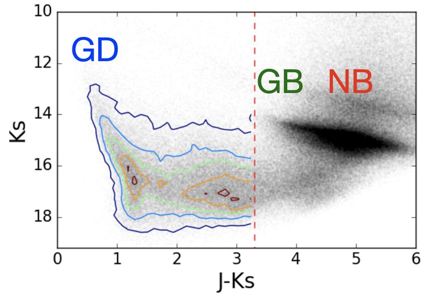
A&A proofs: manuscript no. Nogueras-Lara_et_al

study towards the obscured regions of the Galactic bar (e.g. Gon-
zalez et al. 2011; Minniti et al. 2014), and also permitted the
spiral arm structure to be traced beyond the Galactic bulge (e.g.
Gonzalez et al. 2018; Saito et al. 2020).
    With the present study, we aim to characterise the spiral arms
along the line of sight towards the GC, computing their distance
and the extinction using NIR photometry from the GALACTIC-
NUCLEUS survey (Nogueras-Lara et al. 2018a, 2019a). It is
specially designed to characterise the structure and the stellar
population of the nuclear bulge of the Milky Way with unprece-
dented detail. The high angular resolution of the data and the
fact that it is several magnitudes deeper than any existing NIR
catalogue for the GC (e.g. Nogueras-Lara et al. 2018a, 2019a)
make this survey the best of its kind and the only one that reveals
the details of the structure of the Galactic disc towards this ex-
tremely crowded and highly extinguished line of sight. We also
used the Gaia survey to cross-check our results for the stars be-
longing to the closest spiral arms.

2. Data
For the analysis presented in this paper, we used the GALAC-
TICNUCLEUS catalogue (Nogueras-Lara et al. 2018a, 2019a).
This is a NIR JHK s survey carried out with the HAWK-I instru-
ment (Kissler-Patig et al. 2008) at the ESO VLT unit telescope 4.
It is a single-epoch catalogue consisting of 49 pointings in all
three bands (JHK s ), and includes observations of more than
three million sources in the nuclear stellar disc (NSD), the inner-    Fig. 1. Red giant branch image from the GALACTICNUCLEUS survey
most Galactic bulge, and the transition region between the bulge       (using JHK s bands) showing the regions used in this study. The red
and the NSD. It uses the speckle holography technique (Schödel         arrow marks the position of the supermassive black hole, Sagittarius
et al. 2013) to achieve high angular resolution of ∼ 0.200 , reach-    A* (Sgr A*). The names of the regions are also indicated in the figure:
ing 5 σ detections at J ∼ 22 mag, H ∼ 21 mag, and K s ∼ 21 mag.        central, transition east (TE), transition west (TW), inner bulge south
The survey supersedes all previous photometric surveys for the         (IBS), and inner bulge north (IBN). The distances between the regions
GC region by several magnitudes. The uncertainties on the pho-         correspond to real distances, as indicated by the scaling arrows.
tometry are below 0.05 mag at J ∼ 21 mag, H ∼ 19 mag, and
K s ∼ 18 mag. The zero point (ZP) systematic uncertainty is be-
low 0.04 mag in all three bands.
     As we aim to analyse the stellar population between the
Earth and the GC, we used five regions from GALACTICNU-
CLEUS that correspond to different lines of sight given their
different Galactic latitudes. In particular, we used the central re-
gion, the transition regions east (TE) and west (TW), and the
inner bulge regions north (IBN) and south (IBS). Figure 1 shows
a scheme of the studied area. Given the relatively low number
of stars in the TE, TW, IBS, and IBN regions, we combined the
transition regions and the inner bulge ones to end up with central,
transition, and inner bulge regions.
     The stellar population belonging to the GC is highly red-
dened (e.g. Schödel et al. 2010; Nogueras-Lara et al. 2018a,
2019a), which allows us to clearly distinguish it from the fore-
ground population belonging to the stellar disc using a simple
colour cut (Nogueras-Lara et al. 2020a). Figure 2 shows the
colour-magnitude diagram (CMD) K s versus J − K s of the cen-          Fig. 2. Colour-magnitude diagram K s vs. J − K s from the central region
tral region of the GALACTICNUCLEUS survey. This region al-             of the GALACTICNUCLEUS survey. The red dashed line indicates the
lows us to easily differentiate between the stellar disc and the       colour cut between the stellar population belonging to the GC: Galactic
GC because it is the most extinguished region and the one with         bulge (GB) + Nuclear bulge (NB), and the Galactic disc (GD). The
the largest number of stars in the GALACTICNUCLEUS cata-               contours outline the population belonging to the GD.
logue. The most prominent feature (around K s ∼15, J − K s ∼ 5
mag in the upper panel) corresponds to RC stars belonging to the
GC (see Fig. 14 in Nogueras-Lara et al. 2019a). Namely, the GC         taining to the NB (see Fig. 2 for details). Stars located at redder
stellar population comprises stars from the nuclear bulge (NB,         colours correspond to the Galactic disc. In this way, and as an
e.g. Launhardt et al. 2002; Nogueras-Lara et al. 2020a) and the        initial assumption that is later corroborated by our analysis, the
inner Galactic bulge (e.g. Nogueras-Lara et al. 2018b), the stel-      red dashed line in the figure indicates the approximate colour
lar population of this latter being less reddened than the one per-    division between the foreground population and GC stars.
Article number, page 2 of 17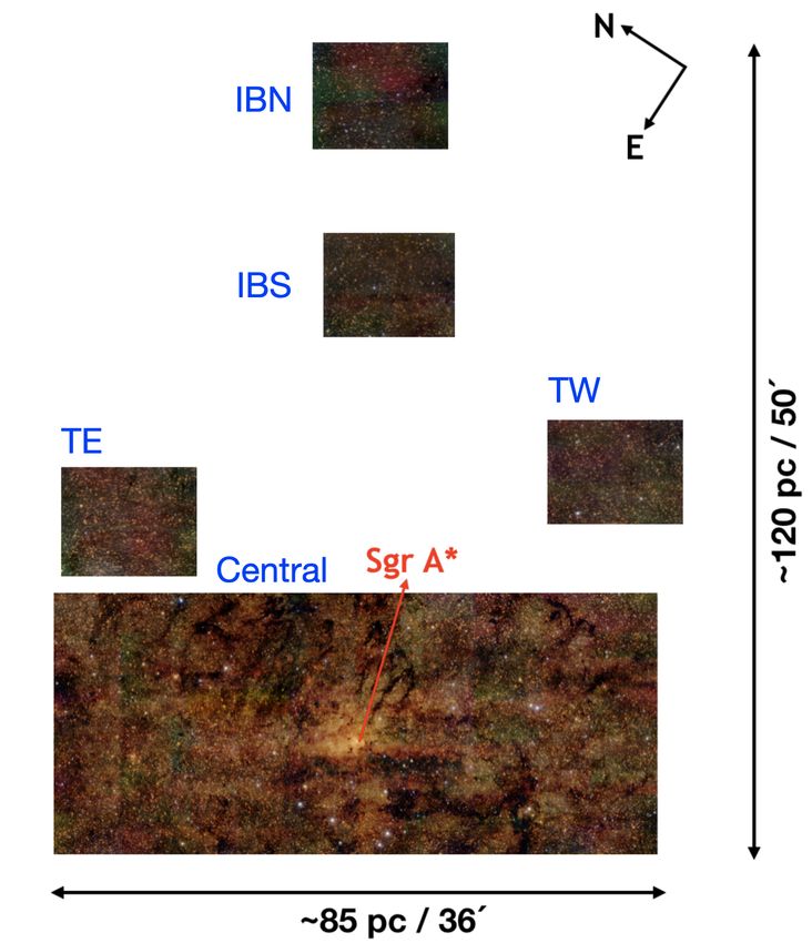
F. Nogueras-Lara et al.: Distance and extinction to the Milky Way spiral arms along the Galactic centre line of sight

3. Colour-magnitude diagram fitting                                         GC extinction of A1.61 µm = 3.40 mag (at ∼ 8 kpc) obtained in
                                                                            Nogueras-Lara et al. (2020b), and assuming that it increases
Previous work using the GALACTICNUCLEUS data suggested                      linearly with the distance from the Earth to the GC. Given the
the presence of spiral arms towards the GC by visual inspection             complexity of the extinction towards the innermost regions of
of the CMDs (e.g. Figs. 14 and 14 from Nogueras-Lara et al.                 the Galaxy (e.g. Nataf et al. 2016; Alonso-García et al. 2017;
2018a, 2019a, respectively). A number of studies based on dif-              Nogueras-Lara et al. 2020b), we used the three-dimensional
ferent spiral arm tracers detect four spiral arms along the line of         extinction maps obtained by Schultheis et al. (2014) to assess
sight towards the GC (e.g. Hou & Han 2014; Vallée 2016; Reid                the assumption of a linear increase in extinction. These authors
et al. 2019). In this way, we analysed our data, constructing a             obtained a steep rise in AKs for different lines of sight near the
simple synthetic model considering the four spiral arms scenario            GC, with a flattening occurring at ∼ 4 − 6 kpc (see their Fig. 8).
as a fiducial model.                                                        The steep behaviour is compatible with the linear increase that
                                                                            we assumed, and it is probably due to the presence of gas and
3.1. Models                                                                 dust in the Galactic disc. On the other hand, the flattening is
                                                                            likely produced by the lower dust and gas content associated
We created synthetic models for each of the spiral arms assum-              to the Galactic bulge in comparison to the Galactic disc (e.g.
ing the star formation history (SFH) derived by Ruiz-Lara et al.            Englmaier & Gerhard 1999). The distance ∼ 4 − 6 kpc was
(2020) for the thin disc in a 2-kpc-radius bubble around the Sun.           obtained using the extinction curve obtained by Nishiyama
In this way, we combined stellar populations of 13, 6, 2, 1, and            et al. (2009) (A J /AKs ∼ 3.02). Using the more recent extinction
0.1 Gyr and scaled them in agreement with the SFH shown in                  curve by Nogueras-Lara et al. (2020b) (A J /AKs ∼ 3.44) would
Fig. 4 of Ruiz-Lara et al. (2020). The metallicity of the models            increase the estimated distance where the flattening occurs by
was selected taking into account the age–metallicity relation for           ∼ 1 kpc, matching our assumption of an upper limit for the
the solar neighbourhood, assuming the mean values for different             contribution of background stars at 5500 kpc from the Earth.
age distributions from Fig. 18 in Feltzing et al. (2001). In par-
ticular, we used [M/H] = −0.07 for all the models except for                    The numbers of stars in each spiral arm were defined as a
the oldest one ([M/H] = −0.28). This metallicity distribution               ratio to the number in the first arm.
is also in agreement with previous studies of the Galactic disc
(Bergemann et al. 2014; Ruiz-Lara et al. 2020).                                 We considered that the observed area increases as the square
    We used PARSEC models (release v1.2S + COLIBRI S_35,                    of the distance, implying that the number of stars is proportional
Bressan et al. 2012; Chen et al. 2014, 2015; Tang et al. 2014;              to the square radius.
Marigo et al. 2017; Pastorelli et al. 2019) and created the syn-
thetic CMDs using the web tool CMD 3.31 . We used the CMD                       We assumed that all the spiral arms have the same width
H versus J −H for the model fitting because in this way we avoid            (∼400 pc from mid-arm to dust lane, Vallée 2014). To simulate
the K s band that is more affected by saturation and crowding than          this, we used a Gaussian with a standard deviation of 400 pc to
the H band. Additionally, using the CMD H versus J − H we can               randomly generate the width effect for each spiral arm.
more clearly separate the different components along the line of
sight because their mean colour differences due to extinction are
                                                                               The extinction to each spiral arm was a free parameter and
significantly larger at J − H than the scatter due to measurement
                                                                            depends on each of the models considered.
uncertainties (Nogueras-Lara et al. 2019a). The model was gen-
erated as follows:
    The main parameters of the model are the distance to each                   After having generated the models, we applied a Gaussian
spiral arm and its associated extinction (d and AH , respectively).         uncertainty distribution to the simulated J and H photometry.
The distance only affects the y-axis of the CMD (the colours                This accounts for the possible differential extinction towards the
are not distance dependent). On the other hand, to compute the              features and also for some possible additional measurement un-
extinction in the J band (A J ) given AH , we used the relation             certainties. For this, we used Gaussians with a standard deviation
AH /A J = 1.87 ± 0.03 obtained by Nogueras-Lara et al. (2020b).             of 0.05 mag.

    We simulated the photometric uncertainties of the data                  3.2. Fitting procedure
assuming a Gaussian distribution with a standard deviation
of 0.05 mag for each of the bands. This value considers the                 For the model fit, we restricted the data to stars that belong to
statistical uncertainties and also the possible ZP variations               the foreground population as indicated in Fig. 2. We only used
(∼0.04 mag) between the different pointings that were combined              the central region, because the lower extinction towards bulge
to get the final photometric catalogue (Nogueras-Lara et al.                and transition regions makes it difficult to separate Galactic disc
2019a).                                                                     stars from GC stars and because the lower number of stars to-
                                                                            wards these regions would lead to lower quality fits. Interstellar
    We simulated a background of stars, whose relative contri-              extinction towards the GC is significantly higher at low latitudes,
bution is a free parameter of the fit. This background follows              which facilitates the separation of disc and GC stars (Schödel
an exponential distribution to account for the Galactic disc                et al. 2014; Nogueras-Lara et al. 2018b).
component. We used a scale length of 2600 pc (Bland-Hawthorn                    We only considered stars with J − H ∈ [0.3, 2.3] and H ∈
& Gerhard 2016) and placed stars at distances between 100                   [10, 18.3] mag, where the completeness in H band is more than
and 5500 pc from the Earth. The interstellar extinction was                 80 % according to Nogueras-Lara et al. (2020b). To estimate the
assumed to linearly increase from AH = 0 (corresponding to                  uncertainty of the fits and to significantly decrease the necessary
0 pc) to AH = 2.025 mag. This value was computed using the                  computing time, we implemented a Monte Carlo (MC) simula-
                                                                            tion creating 500 independent data sets, randomly sampling 5000
1
    http://stev.oapd.inaf.it/cgi-bin/cmd                                    of the accepted stars for each of them.
                                                                                                                      Article number, page 3 of 17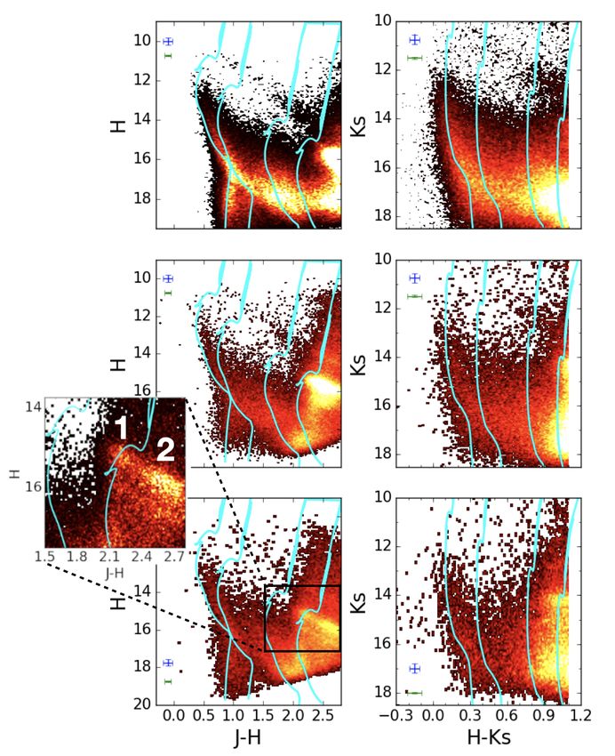
A&A proofs: manuscript no. Nogueras-Lara_et_al

Table 1. Parameters to create the models.                                   parameters in steps of 350 pc to sample the whole parameter
                                                                            space. We defined a grid of AKs in agreement with the AH
                                                                            grid used for the analysis of the CMD H versus J − H. In
             Parameters                                                     this way, we created the models assuming four extinction
            scaling factor        S back = 25, 70, 115, 150%                values for each spiral arm varying from 0.075 to 1.2 mag in
                                                                            steps of 0.075 mag. We also considered the lower K s -band
       d1 =1300, 1650, 2000       AH1 = 0.05, 0.2, 0.35, 0.5                completeness (mainly due to crowding) in comparison to
       d2 = 2350, 2700, 3050 AH2 = 0.65, 0.8, 0.95, 1.1                     the H and J bands used previously (80 % completeness at
                                                                            K s ∼ 16.3 mag, see Nogueras-Lara et al. 2020b). For this,
       d3 = 3400, 3750, 4100 AH3 = 1.25, 1.4, 1.55, 1.7
                                                                            we applied a completeness correction selecting a reference
       d4 = 4450, 4800, 5150 AH4 = 1.85, 2.0, 2.15, 2.3                     level with a completeness of 50 % (K s = 18.3 mag) and
                                                                            randomly removing stars from levels of completeness above
Notes. The scaling factor scales the number of stars of the first           in steps of 1 %, as described in Sect. 3.1.2 of Nogueras-Lara
spiral arm (or the total number of stars in the no-spiral-arms              et al. (2020b). We selected stars fulfilling K s ∈ [11.5, 18.3]
model to the 5000 stars chosen for each simulation). Three dif-             and H − K s ∈ [0, 1.05] to account for the significant satura-
ferent values were tried, scaling the values in steps of 25 % of            tion in K s for stars brighter than 11.5 mag (Nogueras-Lara
the total number of simulated stars. S back refers to the scaling           et al. 2019a) and also to minimise the contamination from
factor of the background population (i.e. stars homogeneously               the inner Galactic bulge (see Fig. 2). We then sampled the
distributed from 100 to 5000 pc with increasing extinction, see             data to create the 500 MC realisations in order to apply the
main text) with respect to the total number of stars belonging to           model fitting. Table 2 shows the results. We concluded that
the spiral arms. di and AHi indicate the distance and extinction to         there is no significant variation in the distance parameters
the i − th spiral arm. The distances and extinctions are given in           within the uncertainties with respect to the results obtained
units of pc and mag, respectively.                                          for the J − H case.

                                                                          – We also analysed the systematic errors due to the chosen bin
     To compare the model with the data, we binned the se-                  width. For this, we repeated the fit varying the bin size of
lected region of the CMD. We used the Python function                       the CMD (±25%). The results are presented in Table A.1 in
numpy.histogram_bin_edges (Harris et al. 2020) to compute the               Appendix A. We did not observe any significant difference
bin widths for each axis. We ended up with 0.09 and 0.18 mag                within the uncertainties.
for the J − H and H axes, respectively.
     We generated a grid of models to fit the MC samples, varying         – We tested the influence of the ZP variability on the results.
the free parameters (see Table 1) and identifying the best ones             We repeated the fit adding and subtracting the ZP uncertainty
via χ2 minimisation. The distance parameters were selected to               (0.04 mag for J and H bands) independently for each band.
homogeneously sample the parameter space in steps of 350 pc.                The results are presented in Table A.2 in Appendix A and
The extinction values also cover the space homogeneously in                 agree well with our results.
steps of 0.15 mag up to an upper limit of 2.3 mag.
     We used the Poisson maximum likelihood parameter χ2 =                – To study the influence of the selected models, we repeated
2Σi mi − ni + ni ln(ni /mi ), where mi is the number of the stars           the analysis using BaSTI models (Pietrinferni et al. 2004,
of the model, ni is the number of stars in the observations, and            2006) to generate the synthetic population described in Sect.
the subindex i indicates the bin of the CMD (e.g. Mighell 1999;             3.1. Because the synthetic population generated using the
Dolphin 2002; Pfuhl et al. 2011). Our grid approach allowed us              BaSTI web tool2 only considers stars with masses larger
to: (1) not have to choose any starting parameters for spiral arm           than 0.5 M , we restricted the lower limit of the H cut to
distances and extinctions, (2) explore the whole parameter space            17 mag instead of 18.3 mag to avoid gaps when analysing
avoiding false minima that might appear when using non-linear               the closest spiral arms. The results are presented in Table
least-squares approaches, and (3) reduce the computing time to              A.3 in Appendix A. We did not observe any significant
make the computation feasible.                                              difference within the uncertainties.

3.3. Properties of the spiral arms                                        – We also tested the possible systematic errors introduced by
                                                                            the chosen SFH. For this, we used a BaSTI (Pietrinferni et al.
We computed the reduced χ2 (χ2red ), considering the fixed pa-              2004, 2006) model that considers a stellar population similar
rameters for each of the MC samples. The minimum χ2red values               to that expected for the local disc according to Rocha-Pinto
from the MC runs show a Gaussian distribution. We obtained a                et al. (2000) as it is implemented in the BaSTI web tool.
mean χ2red = 2.43 ± 0.01, where the uncertainty corresponds to              The selection of the stars was also limited to H = 17 mag
the standard deviation of the values.                                       given the limitations of the BaSTI models. The results are
    Table 2 shows the best solutions for the parameters fixed av-           presented in Table A.3 in Appendix A. We did not observe
eraging over the results obtained for the 500 MC realisations.              any significant difference within the uncertainties.
The uncertainties were obtained considering the maximum be-
tween the standard deviation of the parameter distribution for            – Finally, to check the method, we generated three simulated
each of the 500 MC samples and the half step of the grid (175 pc            data sets considering the same SFH but more realistic situa-
and 0.08 mag, for the distance and the extinction, respectively).           tions. We varied the relative number of stars between arms,
    We addressed the following sources of systematic errors:                the width of the spiral arms, and the relative contribution
                                                                            of the stellar background. We applied the method described
 – We analysed the CMD K s vs. H − K s . We used the synthetic
                                                                      2
   population described in Sect. 3.1 and kept the same distance            http://basti.oa-teramo.inaf.it

Article number, page 4 of 17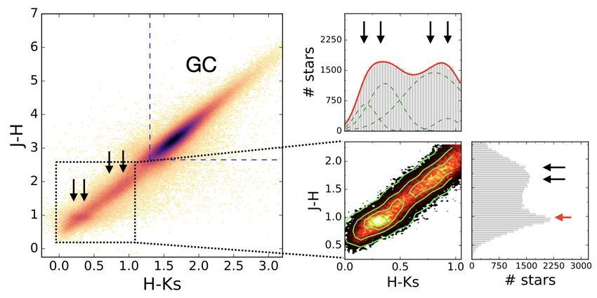
F. Nogueras-Lara et al.: Distance and extinction to the Milky Way spiral arms along the Galactic centre line of sight

Fig. 3. Model fitting performance for a given MC sample (left panel). Middle panel: Best fit for the MC sample (χ2red = 2.24). Right panel:
Residuals after subtracting the model from the data. The colour bar indicates the number of stars per bin using a linear scale.

Table 2. Model fitting results.

                                            JH                                     HK s
                                           d (pc)           AH (mag)              d (pc)           AKs (mag)
                                       1623 ± 175          0.35 ± 0.08         1685 ± 259         0.11 ± 0.04
                                       2641 ± 178          0.77 ± 0.08         2521 ± 205         0.41 ± 0.04
                                       3868 ± 288          1.68 ± 0.08         3420 ± 175         0.90 ± 0.04
                                       4539 ± 198          2.30 ± 0.08         4931 ± 272         1.19 ±0.04
                                   S back = 0.80 ± 0.22                   S back = 0.68 ± 0.20

Notes. The table includes the results corresponding to the CMDs H vs. J − H and K s vs. H − K s . The S back parameter refers to the
scaling factor of the background population (see Table 1). d and AH indicate the distance and extinction to each of the spiral arms.

    previously, now using 100 MC samples. The results are                  3.4. The role of extinction
    presented in Table A.4 of Appendix A. We find that the
    extinction of all the features is always determined within             The extreme extinction towards the GC, in particular towards the
    the uncertainties in all the cases. On the other hand, we              NB (e.g. Nogueras-Lara et al. 2020a), allows us to clearly dis-
    measured some deviation in the results for the distances               tinguish the foreground population and trace the spiral arms as
    of the first simulated spiral arm. The determination of the            shown above. Nevertheless, some contamination from the bulge
    distance is more dependent on the precise shape of the                 is expected for the fourth spiral arm, in particular when using the
    spiral arm features given that it only affects the y-axis (the         K s band. We overcame this difficulty when analysing the J and
    colour, x-axis, does not depend on distance). Thus, it is more         H bands, where the effect of extinction is larger (e.g. Nishiyama
    influenced by the scatter of the data, or by a less defined            et al. 2009), making it easier to distinguish between components
    spiral arm feature. In this sense, the determination of the            with different reddening. Comparing the results with the ones
    distance for the first spiral arm might be more affected               obtained when applying the technique to the CMD K s versus
    because its number of stars is lower in comparison with the            H − K s , allows us to assess the consistency between the distance
    other spiral arms. Nevertheless, the measured deviations are           and extinction results. We ended up with a larger distance for
    always within 1.5 σ. In the case of real data, we believe that         the fourth spiral arm when using the CMD K s versus H − K s ,
    the distance to the first spiral arm is properly determined            although this result remains compatible within the uncertainties
    given the agreement with Gaia (Sect. 4) data and also                  with the results from the CMD H versus J − H (Table 2). There-
    with previous work. It might be possible that the scatter              fore, we conclude that the obtained parameters are not signifi-
    of the data is overestimated when creating the simulations.            cantly affected by this contamination.
    We also measured some deviation when computing the                         A similar analysis is not possible at higher latitudes given
    influence of the background population. Nevertheless this is           the lower extinction towards the Galactic bulge at these lati-
    expected given our simple approach, which is designed to               tudes. The inner bulge fields analysed in Sect. 4 correspond to
    simply identify the extinction and distance to the spiral arms.        an average extinction of AKs ∼ 1.3 mag (averaging over the val-
                                                                           ues obtained by Nogueras-Lara et al. 2018b, for two inner-bulge
                                                                                                                     Article number, page 5 of 17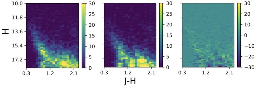
A&A proofs: manuscript no. Nogueras-Lara_et_al

regions located at ∼ 0.6◦ and ∼ 0.4◦ to the Galactic north of
the Milky Way centre), which is only about half of the total ex-
tinction towards the central field (latitude ∼ 0◦ ). Moreover, the
larger size of the central field and the lower density of stars given
the projection effects for higher latitudes also affect the observed
number of stars from the spiral arms in the transition and the
inner bulge regions.
    Therefore, the stars in the third and fourth (and to a certain
degree even the second) spiral arm from the Earth overlap with
the GC stars in the CMDs for the bulge fields. Figure 4 illus-
trates this effect showing the CMDs H versus J − H and K s ver-
sus H − K s for the studied regions. We over-plotted PARSEC
isochrones of 1 Gyr and [M/H] = −0.07 according to the pa-
rameters of distance and extinction obtained for the J − H and
H − K s data of the central region (Table 2). We observed good
agreement between the position of the isochrones and the over-
densities in the CMDs, within the uncertainties. Given the lower
extinction, the features corresponding to the GC are less extin-
guished for the transition and the inner bulge regions than for the
central one. In this sense, the middle and lower panels of Fig. 4
show how the RC features from the inner bulge or the GC stellar
population are contaminated by the presence of stars from the
main sequence belonging to the fourth spiral arm. This effect is
visible in the CMDs H versus J − H, where the RC feature shows
an excess of stars belonging to the isochrone associated to that
spiral arm. The zoomed-in region in Fig. 4, corresponding to the
inner bulge regions, depicts this effect. In this particular case, the
different extinction from the IBN and IBS (Nogueras-Lara et al.
2018b) magnifies the overlap.
                                                                         Fig. 4. CMDs H vs. J − H and K s vs. H − K s for the central, transition,
                                                                         and inner bulge regions of the GALACTICNUCLEUS survey, from the
3.5. Discussion                                                          upper to the lower panels, respectively. The colour code refers to stellar
                                                                         densities, using a power-stretch scale (different in each case to stress
A detailed two-dimensional fit of the experimental CMDs is very          the spiral arm features). Cyan lines correspond to a PARSEC isochrone
complex given the high number of free variables to be consid-            of 1 Gyr and [M/H = −0.07] according to the extinction and distance
ered. Namely, the presence of stars with different ages and/or           parameters obtained for the spiral arm. The blue and green error bars
metallicities, the different contributions from each spiral arm de-      indicate the 1 σ uncertainties of the position of the isochrones and the
pending on its corresponding distance and/or width, the differ-          photometric ZP, respectively. The zoomed-in region corresponds to the
ential extinction, and the possible contamination from the GC            red clump features (e.g. Girardi 2016) from the inner Galactic bulge (‘1’
stellar population for the innermost arms contribute to this in-         and ‘2’ associated to different extinctions from the IBS and IBS regions)
crease in complexity.                                                    and the overlap with the fourth spiral arm.
    Nevertheless, we did not aim to characterise the stellar pop-
ulation and/or metallicities of the analysed stars, but to compute
the distance to the spiral arms and their extinction given the av-       2018). The mean offset between the two catalogues is ∆RA =
erage features in the CMDs. We demonstrate that our method               0.05 ± 0.02 arcsec and ∆Dec = 0.04 ± 0.02 arcsec. We defined a
is good enough for our purposes, addressing potential sources            maximum distance of ∼ 0.1500 to cross-correlate the catalogues.
of systematic errors and trying different stellar populations and        Moreover, we only accepted stars whose distances was mea-
models. Our results agree well with the distances from the recent        sured with more than 3 σ significance, and removed all the stars
work by Reid et al. (2019). From Fig. 1 of this latter paper we          with distances larger than 10 000 pc. In this way, we avoid er-
obtained d1 ∼ 1.4, d2 ∼ 2.7, d3 ∼ 3.7, and d4 ∼ 4.7 kpc, which           roneous identifications and stars with spurious astrometric solu-
are fully compatible with our results.                                   tions (Gaia Collaboration et al. 2018).
    The obtained structures would correspond to the Sagittar-
ius–Carina, the Scutum–Centaurus–OSC, the Norma–Outer, and                   The high extinction towards the GC and the optical pho-
the 3 kpc arms. As reference values for the distance towards the         tometry from Gaia only allowed us to obtain common stars
spiral arms, we used the results obtained for the CMD H versus           whose colours are restricted to J − H . 1 mag for faint stars
J − H because of the lower contamination from the GC and also            (H . 16 mag) and J − H . 1.5 mag for some bright stars around
because the shape of the isochrones is more sensitive to changes         H . 12 mag. To obtain the distances to the detected common
in the y-axis as can be seen in Fig. 4.                                  stars, we used the Gaia parallaxes taking into account that, in
                                                                         general, they cannot be directly inverted to get the distance to
                                                                         a given source (e.g. Luri et al. 2018; Bailer-Jones et al. 2018).
4. Analysis of Gaia sources                                              We applied the near-linear trend of distance bias (δ p = −0.054)
                                                                         derived by Schönrich et al. (2019). To remove any additional
To cross-check the obtained distances to the spiral arms, we             problem related to the distance to individual stars, we computed
cross-correlated the regions from the GALACTICNUCLEUS                    average distances building histograms of the underlying distri-
survey with the Gaia DR2 catalogue (Gaia Collaboration et al.            butions corresponding to each of the analysed regions (Fig. 5).
Article number, page 6 of 17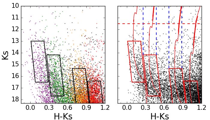
F. Nogueras-Lara et al.: Distance and extinction to the Milky Way spiral arms along the Galactic centre line of sight

We ended up with ∼ 5000, ∼ 800, and ∼ 400 stars for the central,
transition, and inner bulge regions, respectively.
    Given the high extinction along the line of sight towards the                     350
GC, we can only detect stars located at . 3kpc from Earth us-                         300                         d1 = 1.69 ± 0.04
ing Gaia data for this line of sight, restricting the analysis to the
closest spiral arms. We detected a bimodal distribution that can                      250                          d2 = 3.08 ± 0.16

                                                                            # stars
be fitted well with a two-Gaussian model. We computed the aver-
age distance to each of the features as the mean value of each of                     200
the Gaussians. The uncertainties were estimated considering the                       150
error of the mean. The results and the associated uncertainties
are over-plotted in Fig. 5. We find that the two-Gaussian distri-                     100
bution fits the data better than a single Gaussian when selecting
stars with distances of < 5000 pc and using the SCIKIT-LEARN                           50
Python function GaussianMixture (GMM Pedregosa et al. 2011)                             0
to compute the Bayesian information criterion (Schwarz 1978)
and the Akaike information criterion (Akaike 1974). We find that
the two-Gaussian distribution is preferred. We did not try any                        120
more complex models because of the low completeness of the
                                                                                      100                         d1 = 1.53 ± 0.06
data beyond 3000 pc, and so no more components are expected                                                        d2 = 2.82 ± 0.26
(nor visually identified) in the distributions.
                                                                                       80

                                                                            # stars
    Our results agree well with the presence of two spiral arms,
particularly in the case of the central and the transition regions,
where the number of stars is larger than for the inner bulge, and
                                                                                       60
where the distance values obtained are somewhat smaller. The
secondary Gaussian feature is significantly smaller than the first
                                                                                       40
one, as expected. This is because only a small fraction of the stars                   20
belonging to the second spiral arm were detected in the Gaia sur-
vey given the extinction and the larger distance. We computed a                         0
mean value for the distance to each of the features averaging over
the obtained results and ended up with d1_Gaia = 1.5 ± 0.1 kpc
and d2_Gaia = 2.8 ± 0.2 kpc. The uncertainties refer to the stan-                       80
dard deviation of the measurements towards the three different                          70                        d1 = 1.38 ± 0.06
regions. The obtained results agree within the uncertainties with
                                                                                        60                         d2 = 2.55 ± 0.25
the distances obtained for the first and the second spiral arms in
                                                                                        50
                                                                              # stars

the previous section and in the literature (see Sect. 1).
                                                                                        40
5. Analysis of the colour–colour diagram                                                30
Figure 6 shows the colour–colour diagram (CCD) J − H ver-                               20
sus H − K s of the central region of the GALACTICNUCLEUS
survey. The highest density region in the CCD (H − K s > 1.3
                                                                                        10
mag and J − H > 2.65 mag) corresponds to the GC. These are                               0
                                                                                             0     2000         4000        6000        8000
                                                                                                      distance (pc)
stars from the NB and the inner Galactic bulge. Excluding these,
there are two main over-density features (J − H ∼ 1 mag and
J − H ∼ 1.8 mag) that can be identified in the right panel of Fig.
6. According to the analyses carried out in the previous sections,
these overdensities correspond to the spiral arm structure along
the line of sight from the Earth to the GC. We built histograms           Fig. 5. Histograms of the distances to the common stars between Gaia
of the J − H and H − K s distributions to further analyse these           and GALACTICNUCLEUS detected in the central, transition, and inner
                                                                          bulge regions (upper, middle, and lower panel, respectively). The solid
features (right panels in Fig. 6):                                        green lines indicate the two-Gaussian fits, whereas the red and cyan
                                                                          dashed lines show each of the two Gaussian components. The mean
 – J − H: Given the overlap between the isochrones corre-                 values and their errors for each component are indicated for each panel
   sponding to the first and the second spiral arms that we               in units of kpc.
   observed in the CMDs H versus J − H (left panels Fig.
   4), it is not possible to distinguish the four spiral arms in
   the histogram corresponding to the J − H distribution. We
   observed a prominent narrow peak around J − H ∼ 1 mag
   and a secondary extended peak around J − H ∼ 1.75 mag.                  – H − K s : There are two clear features that probably corre-
   According to the synthetic CMD fitting, the first peak is                 spond to the overlap between the first and second, and third
   probably the result of the overlap between the first and the              and fourth spiral arms. Given that the overlap between the
   second spiral arms. On the other hand, the extended peak                  isochrones of the spiral arms is not as significant as for
   might be the result of the overlap between the third and the              J − H (see Fig. 4), we tried to fit this histogram using a four-
   fourth spiral arms.                                                       Gaussian model to check whether it is compatible with the
                                                                             structure obtained previously. This is a simplistic approach
                                                                                                                    Article number, page 7 of 17
A&A proofs: manuscript no. Nogueras-Lara_et_al
Fig. 6. Left panel: Colour–colour diagram J − H vs. H − K s corresponding to the central region of the GALACTICNUCLEUS survey. The black
arrows indicate the over-density features that correspond to the spiral arms detected in Sect. 3. The blue dashed lines mark the stellar population
belonging to the GC, where the density is significantly different from the rest. Right panel: Zoom into the foreground population from the spiral
arms and histograms corresponding to the underlying distributions. The red solid line indicates the result of a four-Gaussian fit (green dashed lines
for each individual Gaussian). The black arrows show the mean location of the spiral arms. The red arrow indicates the overlap between the first
and the second spiral arms in one single feature in the histogram J − H.
that only attempts to detect over-densities associated to the We only used the central region to analyse the extinction for
spiral arms in the CCD. two reasons: (1) The average extinction of the GC stellar popu-
We used the stars detected in all three bands (JHK s ) within lation is maximum for this region, allowing us to detect the in-
the same magnitude ranges used in Sect. 3 for the analysis nermost spiral arms. (2) The number of available reference stars
of the CMDs H versus J − H and K s versus H − K s . We is largest given the covered area, which implies that more stars
fitted the model using the Python SCIPY routine curve-fit are available to analyse the extinction.
and the initial values according to the expected positions of To select the reference stars belonging to each of the spiral
the spiral arm features. We only imposed that the four Gaus- arms, we generated a synthetic stellar population according to
sians cannot take negative values for the fit. We obtained that the best fit obtained for the CMD K s versus H−K s (see Sect. 3.3).
this simple model agrees well with the results from previ- The synthetic model indicates the regions where the probability
ous sections. We obtained mean values of (H − K s )1 ∼ 0.2, of finding stars from a given spiral arm is maximum. In this way,
(H − K s )2 ∼ 0.4, (H − K s )3 ∼ 0.8, and (H − K s )4 ∼ 0.9 we defined a selection box to identify them in the real data (left
mag, where the subindex indicates the number of each spi- panel of Fig. 7 ). Figure 7 shows the chosen stars with which we
ral arm. The feature corresponding to the fourth spiral arm is analyse the extinction.
smaller than the others. Nevertheless, this is expected given
the colour cuts applied to limit possible confusion with the
stars belonging to the inner Galactic bulge, whose extinction 6.1. Extinction curve
is close to that from this spiral arm (Nogueras-Lara et al.
2018b). We computed the ratios between extinctions A J /AH and AH /AKs
using the selected stars belonging to the spiral arms, and then
Therefore, the analysis of the CCD allows us to distinguish used these ratios to derive the extinction curve. To select the ref-
between GC and spiral arm stellar populations and agrees with erence stars in the J band avoiding the overlap of the spiral arm
the structure derived previously. features (see Fig. 7), we used the reference stars in the CMD K s
versus H − K s that were also detected in J. To calculate the ex-
tinctions Ai (where i indicates the photometric band), we com-
6. Extinction puted the intrinsic colours (J − H and H − K s ) of each of the
According to the previous analysis, we find that the CMD K s reference stars interpolating from a PARSEC isochrone (Fig. 7)
versus H − K s is the best choice to select the reference stars with corresponding to the best-fit parameters obtained in Sect. 3.
which to analyse the extinction corresponding to each feature. Given the completeness due to crowding of the K s -band data,
This is because the stellar population belonging to each spiral we applied a completeness correction as explained in Sect. 3.3.
arm can be disentangled more easily there than in the CMD us- As this approach is based on the removal of stars above a refer-
ing the J band, where the isochrones from different spiral arms ence completeness limit of 50 %, we generated 100 MC samples,
overlap (see Fig. 4). randomly removing stars to correct for completeness (see Sect.
Article number, page 8 of 17F. Nogueras-Lara et al.: Distance and extinction to the Milky Way spiral arms along the Galactic centre line of sight
Table 3. Extinction curve using spiral arm reference stars.
# spiral arm A J /AH AH /AKs
1 2.07±0.31 1.94±0.39
2 1.89±0.21 1.83±0.21
3 1.89±0.19 1.86±0.19
4 1.82±0.19 1.87±0.19
Mean value 1.89±0.11 1.86±0.11
Fig. 7. Colour–magnitude diagrams K s vs. H − K s . Left panel: Best
model-fit solution obtained for the CMD K s vs. H − K s (see Table 2). Notes. The mean values in the last row correspond to a weighted
Different colours indicate the stars contributing from each of the spi- mean of the extinction ratios obtained for the spiral arms in the
ral arms. In particular, purple, green, orange, red, and black dots indi-
cate stars from the first, second, third, and fourth spiral arms, and back-
rows above.
ground sources respectively. Black solid parallelograms mark the selec-
tion of reference (mainly main-sequence) stars to analyse the extinction et al. 2011; Alonso-García et al. 2017), as discussed in Sect. 7
corresponding to each of the spiral arms. Right panel: Real data consid- in Nogueras-Lara et al. (2020b).
ering completeness correction as indicated in Sect. 3.3. The red dashed These values are in agreement with the results obtained for
line indicates the saturation limit of the K s photometry (K s = 11.5 mag).
the GC (A J /AH = 1.87 ± 0.03 and AH /AKs = 1.84 ± 0.03) by
The red solid parallelograms depict the reference main sequence stars
according to the best model fit as shown in the left panel. The isochrones Nogueras-Lara et al. (2020b). The constant extinction ratios for
corresponding to a stellar population of 1 Gyr and [M/H] = −0.07 are stars belonging to different structures and distances indicate that
over-plotted in red (see Sect. 3.3). The blue dashed lines indicate the the extinction curve in the NIR bands JHK s towards the GC
stars added to the reference main sequence stars to create a K s luminos- does not vary significantly with distance. Therefore, the extinc-
ity function for the second and third features (see Sect. 7). tion law obtained for the GC (e.g. Nogueras-Lara et al. 2019b,
2020b) is also applicable when studying the foreground popula-
tion corresponding to the spiral arm structure from the Earth to
3.1.2 of Nogueras-Lara et al. (2020b) for further details). We the GC.
computed the ratios between extinctions following the equation:
6.2. Extinction maps
i − j − (i − j)0
Ai /A j = +1 , (1) Once we had determined the spiral arm structure, we built K s -
ext j extinction maps corresponding to each of the spiral arms in order
to further analyse how the extinction varies along the line of sight
where i and j are the photometric bands, the subindex ‘0’ indi- towards the GC. We used all the available stars within the selec-
cates intrinsic colour and ext j is the mean extinction to a spi- tion box without applying the completeness correction. This is
ral arm as indicated in Table 2. We averaged over all the refer- because detecting less stars due to completeness problems will
ence stars for a given spiral arm and computed the uncertainties not influence the values of the extinction. On the contrary, using
quadratically propagating the uncertainties corresponding to the all the stars allows us to increase the number of reference stars
magnitudes involved in Eq. 1. In particular, we considered the to improve the quality of the extinction maps.
ZP systematic uncertainty of 0.04 mag for each band in the cal-
culation, and the uncertainty of the mean extinction to a given
spiral arm. 6.2.1. Methodology
We obtained the final values and uncertainties as the mean We built the extinction maps using stars within the reference
of the individual results of each of the 100 MC iterations. Ta- boxes shown in Fig. 7. We converted the observed stellar colour
ble 3 summarises the results. We find that the extinction ratios H − K s into extinction following the equation:
A J /AH and AH /AKs do not vary for the different spiral arms
considered, within the uncertainties. We used a weighted mean
to compute mean values of the ratios taking into account the H − K s − (H − K s )0
extKs = , (2)
larger uncertainties obtained for the first spiral arm, where the AH /AKs − 1
lower number of stars and the possible contamination by stars
close to the Sun might influence the results. We ended up with where H and K s are the observed magnitudes, AH /AKs is the
A J /AH = 1.89 ± 0.11 and AH /AKs = 1.86 ± 0.11. These val- relation between extinctions obtained in Nogueras-Lara et al.
ues are in agreement with the recent results obtained for the GC (2020b) and is equal to 1.84 ± 0.03, and (H − K s )0 refers to
(A J /AH = 1.87 ± 0.03 and AH /AKs = 1.84 ± 0.03) by Nogueras- the intrinsic colour, computed for each star interpolating from
Lara et al. (2019b, 2020b). Therefore, our results point towards a PARSEC isochrone as explained in Sect. 6.1. Equation 2 was
a more complex extinction curve in the NIR than the simple adapted from Eq. 5 in Nogueras-Lara et al. (2018a) to avoid us-
power-law approach that is generally accepted (e.g. Nishiyama ing the effective wavelengths, given that they vary for different
et al. 2006). This more complex behaviour of the extinction stellar types and extinctions (e.g. Nogueras-Lara et al. 2020b).
curve might explain the different values obtained in the liter- To create the extinction maps, we applied the approach de-
ature (e.g Nishiyama et al. 2009; Stead & Hoare 2009; Fritz scribed in Nogueras-Lara et al. (2018a, 2020a), but using the
Article number, page 9 of 17A&A proofs: manuscript no. Nogueras-Lara_et_al
Table 4. Extinction values from the extinction maps. 6.2.2. Inter-arm extinction
We computed the differential extinction per kiloparsec (AKs /d)
for each of the spiral arms. We used the results from Table 4 and
the distances to each of the spiral arms obtained in Sect. 3.5. We
Spiral # reference AK s ∆ stat ∆ syst find 0.07±0.01, 0.28±0.07, 0.43±0.12, and 0.45±0.24 mag/kpc
arm stars (mag) (mag) (mag) for each of the spiral arms, from the closest to the furthest, re-
spectively. The uncertainties were computed quadratically prop-
1 7756 0.12 0.02 0.06 agating the uncertainties of the AK s and the distances. As the
2 13468 0.40 0.02 0.07 main goal is to compare the differential extinction per kiloparsec
3 19594 0.93 0.02 0.07 for the spiral arms, we did not consider the systematic uncer-
tainty of AKs because it would influence all the measurements in
4 24405 1.23 0.01 0.09 the same direction (adding them would increase the uncertain-
ties of AKs /d up to 0.04, 0.11, 0.14, and 0.29 mag/kpc). Figure
10 shows the relation between the extinction and the distance to
Notes. Column #reference stars indicates the number of refer- a given spiral arm. The red dashed lines join the experimental
ence stars used to create the maps. AKs indicates the mean value points and correspond to linear fits between consecutive spiral
obtained for the stars in the selection boxes in Fig. 7. ∆ stat and arms, whose slope is the differential extinction per kiloparsec
∆ syst refer to the statistical and systematic uncertainty. computed previously.
We find an increase in the differential extinction per kilopar-
sec along the line of sight towards the GC. We also find that
reference stars previously specified instead of RC stars. Namely, the increase in ratio (ri, j = (AKs /d)i /(AKs /d) j ) between consec-
we defined a pixel size of 2000 (larger than in the Nogueras-Lara utive arms (i, j) is r1,2 = 4.00 ± 0.07, r2,3 = 1.54 ± 0.24, and
et al. (2018a, 2020a) given the significantly lower number of ref- r3,4 = 1.04±0.58. This might indicate an increase in material be-
erence stars, and the significantly lower influence of the differ- tween arms that would be in agreement with the exponential thin
ential extinction for the spiral arm than for the GC stellar popu- disc of the Milky Way (e.g. Bland-Hawthorn & Gerhard 2016).
lation), and computed the extinction for each pixel using at least Other possibilities, such as different grain composition of the in-
five reference stars within a radius of 3000 from the centre of terstellar dust, and/or different spiral arm width for the observed
each pixel. We also applied an inverse distance weight method line of sight, might also be possible. A number of recent studies
(p = 0.25) to consider the different distances of each reference aim at analysing the dust distribution along the Galactic plane
star to the centre of the pixel (see Sect. 7 of Nogueras-Lara et al. (e.g. Rezaei Kh. et al. 2018; Green et al. 2019; Lallement et al.
(2018a) for further details). We computed the statistical uncer- 2019; Hottier et al. 2020). These are normally limited by a 3 kpc
tainties considering the variation of the extinction for a given sphere imposed by the limitations of the second release of the
pixel using a jackknife algorithm. Moreover, we estimated the Gaia survey. Nevertheless, we can compare their findings with
systematic uncertainty taking into account the uncertainties of our results for the closest spiral arms. Although the dust distribu-
AH /AKs and the ZP systematic uncertainty (0.04 mag for both H tion seems to be very patchy and does not obviously follow con-
and K s bands Nogueras-Lara et al. 2019a). tinuous spiral arm footprints, it is possible to see an increase in
Figure 8 and Table 4 show the results. We obtained that the extinction in the line of sight towards the GC (see Fig. 7 in Hot-
extinction maps for the different spiral arms are quite homoge- tier et al. 2020) and an increase in dust density (Fig. 4 in Rezaei
neous and do not present any significant extinction variations. Kh. et al. 2018), which might be in agreement with our results.
The largest variations are measured for the first spiral arm, where Deeper photometry and distance measurements are needed for a
the lower number of stars and the possible influence of stars in more sensitive analysis of the innermost regions of the Galactic
the vicinity of the Sun (introducing large differential distances disc. Our analysis and the GALACTICNUCLEUS survey might
between the stars within this map) might contaminate our re- be useful for the next steps in tracing and measuring the dust dis-
sults. Moreover, the lower value of the mean extinction for the tribution and extinction along the line of sight towards the GC.
first layer makes any relative difference more visible due to the
denominator of Eq. 2.
To check the homogeneity of the derived extinction layers, 7. Stellar population analysis
Fig. 9 shows histograms of the extinction computed for the spi- 7.1. Luminosity function
ral arm reference stars using the corresponding extinction maps.
We obtained that a Gaussian model properly fits the data for all We created de-reddened K s -luminosity functions (KLFs) and fit-
of the spiral arms. The standard deviations of the distributions ted them with a linear combination of theoretical luminosity
(over-plotted in Fig. 9) are similar in all the cases, but are some- functions (Parsec models) to determine the stellar population
what larger for the first spiral arm as expected given the reasons and the SFH of the detected spiral arm features. The analysis
explained above. We concluded that the extinction is homoge- of the KLFs is based on the relative weight of the main features
neous within each spiral arm feature and that there is no overlap appearing on the luminosity functions, such as the RC, the red
between them. Therefore, they appear to be independent extinc- giant branch bump, or the asymptotic giant branch bump (e.g.
tion layers. We also compared them with an extinction map ob- Nogueras-Lara et al. 2020a; Schödel et al. 2020). Given that the
tained for a region of the NB (Nogueras-Lara et al. 2020a). In uncertainties of the luminosity functions are proportionally re-
this case, the Gaussian fit is not adequate given the inhomogene- lated to the detected number of stars (∼ #stars1/2 ), a sufficient
ity and the larger extinction variations within the line of sight. On number of stars is needed to apply the proposed methodology.
the other hand, we compared the mean values obtained in Table 4 Therefore, we excluded the first spiral arm from the analysis.
with the results from the analysis of the CMD K s versus H − K s Moreover, some contamination from the Galactic bulge might
(Table 2) and checked that they agree within the uncertainties. affect the fourth spiral arm given the proximity in extinction and
Article number, page 10 of 17F. Nogueras-Lara et al.: Distance and extinction to the Milky Way spiral arms along the Galactic centre line of sight
Fig. 8. Left column: Extinction maps corresponding to each spiral arm. Right column: Associated uncertainties obtained using a jackknife algo-
rithm (see main text for further details). White pixels indicate regions where the number of reference stars is not enough to compute an extinction
value. The white rectangle in the upper part of the fourth spiral arm corresponds to a region of poor quality data in H band (see Table A.1. in
Nogueras-Lara et al. 2019a). Given the increase in extinction for further spiral arms, the colour scale is different for each of the extinction maps.
The extinction range is always the same, 0.35 mag, in order to make small extinction variations within the same extinction layer visible.
the use of the CMD K s versus H − K s , to select the stars belong- rardi 2016), are very useful for disentangling the different stellar
ing to each spiral arm. Hence, we restricted the analysis to the populations (e.g. Nogueras-Lara et al. 2018b, 2020a).
second and the third spiral arms. We corrected the reddening, applying the extinction maps
First of all, to correct possible saturation problems and also derived previously for the corresponding spiral arms (Sect. 6.2).
include stars with K s < 11.5 mag, we used the SIRIUS IRSF The KLFs were computed selecting the bin-width using the
catalogue (e.g. Nagayama et al. 2003; Nishiyama et al. 2006) to Python function numpy.histogram (Harris et al. 2020). We
replace the K s photometry of stars with K s < 11.5 mag. We ac- used the completeness solution due to crowding obtained in
counted for possible deviations of the ZP, correcting the photom- Nogueras-Lara et al. (2020b) for the K s band. We limited the
etry from SIRIUS with respect to non-saturated common bright correction to magnitudes where the completeness is > 70%.
stars between both catalogues. We also included the photometry To fit the KLFs, we used a similar approach as in Nogueras-
of bright stars that were not detected in K s band in the GALAC- Lara et al. (2020a); Schödel et al. (2020). We generated 1000
TICNUCLEUS catalogue because of saturation. We selected MC samples from the original KLFs, assuming Gaussian uncer-
stars within the boxes used to create the extinction maps and tainties and fit them with a linear combination of 14 theoretical
also included the stars belonging to the ascending giant branch PARSEC luminosity functions3 . We used the following models
following the isochrones, as indicated by the blue dashed lines (assuming metallicities in agreement with Feltzing et al. (2001)
in Fig. 7. We established a lower limit of K s = 9 mag to account for the different ages, as in previous sections, and a Kroupa ini-
for the saturation of the SIRIUS survey (Matsunaga et al. 2009). tial mass function) to sample the age space: 12, 9, 7, 5, 3, 2, 1,
In this way, we are able to include more red giant stars whose
3
main features in the KLF, in particular the RC feature (e.g. Gi- http://stev.oapd.inaf.it/cgi-bin/cmd
Article number, page 11 of 17You can also read