Delineating urban park catchment areas using mobile phone data: A case study of Tokyo - Unpaywall
←
→
Page content transcription
If your browser does not render page correctly, please read the page content below
Delineating urban park catchment
               areas using mobile phone
               data: A case study of Tokyo
                  The Harvard community has made this
               article openly available. Please share how
               this access benefits you. Your story matters

Citation              Guan, ChengHe, Jihoon Song, Michael Keith, Yuki Akiyama, Ryosuke
                      Shibasaki, Taisei Sato. 2020. Delineating urban park catchment
                      areas using mobile phone data: A case study of Tokyo. Computers
                      Environment and Urban Systems. 81: 101474

Published Version     10.1016/j.compenvurbsys.2020.101474

Citable link          http://nrs.harvard.edu/urn-3:HUL.InstRepos:42652467

Terms of Use          This article was downloaded from Harvard University’s DASH
                      repository, and is made available under the terms and conditions
                      applicable to Open Access Policy Articles, as set forth at http://
                      nrs.harvard.edu/urn-3:HUL.InstRepos:dash.current.terms-of-
                      use#OAP
Delineating urban park catchment areas using mobile phone data: A case
study of Tokyo
ChengHe Guan12*, Jihoon Song34, Michael Keith2, Yuki Akiyama3, Ryosuke Shibasaki3, Taisei
Sato5
1
  NYU Shanghai, China
2
  PEAK, Centre on Migration, Policy and Society, University of Oxford, UK
3
  Center for Spatial Information Science, University of Tokyo, Japan
4
  Harvard-China Project on Energy, Economy, and Environment, Harvard University
5
  ZENRIN-Datacom CO., LTD., Japan
* Corresponding author’s email: chenghe.guan@nyu.edu

Abstract
Urban parks can offer both physical and psychological health benefits to urban dwellers and
provide social, economic, and environmental benefits to society. Earlier research on the usage of
urban parks relied on fixed distance or walking time to delineate urban park catchment areas.
However, actual catchment areas can be affected by many factors other than park surface areas,
such as social capital cultivation, cultural adaptation, climate and seasonal variation, and park
function and facilities provided. This study advanced this method by using mobile phone data to
delineate urban park catchment area. The study area is the 23 special wards of Tokyo or
tokubetsu-ku, the core of the capital of Japan. The location data of over 1 million anonymous
mobile phone users was collected in 2011. The results show that: (1) the park catchment areas
vary significantly by park surface areas: people use smaller parks nearby but also travel further
to larger parks; (2) even for the parks in the same size category, there are notable differences in
the spatial pattern of visitors, which cannot be simply summarized with average distance or
catchment radius; and (3) almost all the parks, regardless of its size and function, had the highest
user density right around the vicinity, exemplified by the density-distance function closely
follow a decay trend line within 1-2 km radius of the park. As such, this study used the density
threshold and density-distance function to measure park catchment. We concluded that the
application of mobile phone location data can improve our understanding of an urban park
catchment area, provide useful information and methods to analyze the usage of urban parks, and
can aid in the planning and policy-making of urban parks.

Keywords: Urban park catchment area; Geocoded Mobile Data; Urban big data; Urban green
systems; Tokyo

Acknowledgement and Funding
This article was sponsored by the Shanghai Pujiang Program, Grant Ref: 2019PJC076;
completed with support from the PEAK Urban programme, funded by UKRI’s Global Challenge
Research Fund, Grant Ref: ES/P01105 5/1. This authors received support from the Harvard-
China Project of Harvard University, the Shanghai Key Lab for Urban Ecological Processes and
Eco-Restoration of East China Normal University, and the Zaanheh Project fund and Center for
Data Science and Artificial Intelligence at NYU Shanghai.

                                                 1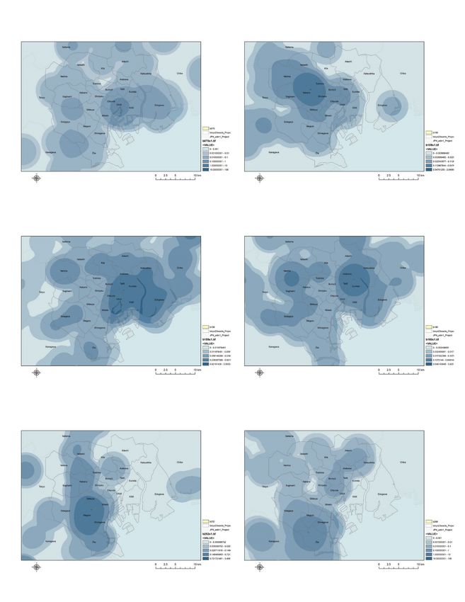
1. Introduction
    Urban parks provide both physical and psychological health benefits to each individual urban
dweller and provide social, economic, and environmental benefits to society (Chiesura, 2004;
Bedimo-Rung et al, 2005; Xu et al., 2019). These benefits include encouraging physical
activities, increasing property value, enhancing ecological biodiversity, and cultivating social
capital and interaction (Pickett et al., 2016; Xiao et al, 2019). On the other hand, planning urban
parks without spatial integration can also introduce negative impacts such as spatial access
inequity (Chang and Liao, 2011), public service disparity (Wolch et al., 2014), and gentrification
(Zhai et al, 2018). A deeper understanding of the catchment area of urban parks – the area from
which a park attracts a population that uses its services - is essential to the allocation of public
amenities such as parks and can ultimately influence the healthy development of urban areas
(Ratti et al., 2006; Rios and Munoz, 2017; Zhai et al, 2018).
    Since early 21st century, the emergence of urban big data has provided considerable
opportunity to examine urban mobility and the use of public amenities at a lower cost, larger
scale, and higher efficiency (Evans-Cowley and Kitchen, 2011; Cao et al, 2015; Rios and
Munoz, 2017; Riggs and Gordon, 2018; Xiao et al., 2019). For example, social media data,
crowdsourcing data, traffic and vehicular data have been extensively used to analyze urban space
and activities (Evans-Cowley and Kitchen, 2011; Cao et al, 2015; Zhai et al, 2019). Among the
different types of urban big data, mobile application data can be used to support a variety of
planning activities and research objectives. For example, Riggs and Gordon (2018) provide a
taxonomy to define how the application of mobile phone data can change planning and local
policy making. Xiao et al (2019) explored the disparities in park access through mobile phone
data. However, using mobile phone data to understand the usage of urban parks remains
understudied.
    This study uses mobile application data to delineate urban park catchment areas in the 23
special wards of Tokyo or tokubetsu-ku, the core of the capital of Japan. The location data of
over 1 million anonymous mobile phone users was collected from January 1 to December 31,
2011. The mobile phone users’ residential location and distance to the urban parks they visited
was identified and tracked using the data. We propose to answer the following questions: (1)
What are the spatial patterns of urban park catchment area (UPCA) 1 using the geocoded mobile
data (GMD)? (2) Can the density gradient of UPCA reveal systematic variations by park area?
(3) What innovative spatial parameters can improve our understanding of UPCA?
    The rest of the paper is organized as follows: The literature review section briefly introduces
the conventional methods and the mobile phone data application of measuring urban park
catchment area. The methodology section presents the application of mobile signaling data in
park catchment area delineation before analyzing the results. The concluding section discusses
urban park planning policy interventions using mobile phone data and the challenges and
opportunities of such an application for delineating UPCA.

2. Literature review
2.1. Conventional approaches for park catchment area estimation and park planning

1
    Catchment area and service area, in this paper, are used interchangeably.

                                                            2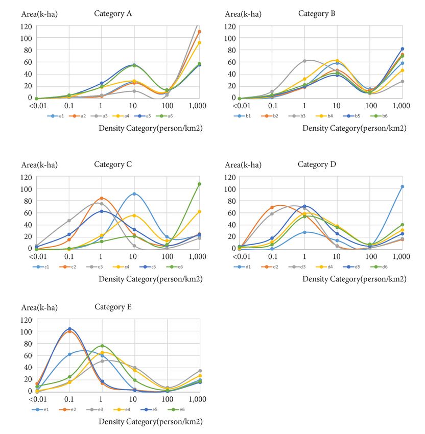
Earlier research relied on distance or walking time from residential location as the most
important precondition for use of green spaces to delineate UPCA (Grahn and Stigsdotter, 2003;
van Herzele and Wiedemann, 2003; Wolch et al., 2014). For example, according to most
researchers, neighborhood parks should be situated within a five-minute walk, corresponding to a
maximum 400m radius from a user’s residence, if they are to be perceived as accessible (Perry,
1929; Xiao et al, 2019). Other studies have proposed planning and design guidelines for urban
parks that ought to adhere to a hierarchical system of standards, where each class of parks has a
different walkable catchment area, partly determined by its size (Gobster, 2002; van Herzele and
Wiedemann, 2003; Giles-Corti et al., 2005; Ahas et al., 2010; Dai, 2011; Wolch et al., 2014;
Reyes et al., 2014).
   In Belgium, for instance, standard of local park authorities recommended a 5 ha minimum
surface area and a catchment radius of 800 m for a neighborhood quarter park and 10 ha and a
1,600 m for a district park (Herzele and Wiedemann, 2003). The U.S. community parks of 6 ha
or more should have a catchment radius of 400-800 m and city parks cover a one-hour driving
radius (Lancaster, 1983). A community park is considered to serve 1,000 people per 1-2 acres up
to 5,000 and a city park to serve 1,000 people per 5-6 acres (National Recreation and Park
Association, 1995). In some more densely populated cities in Asia, there are similar distance-
based regulations on catchment areas. For example, the Bangladesh regulation calls for local and
neighborhood parks services for frequent visits within a walking distance of 400 m (Jafrin and
Beza, 2018). In China, the parks guideline recommends that the service radius of district parks
and neighborhood parks should be between 300-500 m and 500-1000 m, respectively (Zhai et al,
2018).
   Requirements and recommendations for park environment and facilities are often provided in
conjunction with the assumed park catchment size. Marcus and Francis (2003) offered an
expansive list of user groups, activity types, and design recommendations for general
neighborhood parks. For smaller mini parks and pocket parks, it assumed most of the park users
come from within four residential blocks. Hence, the recommendation for those park types
emphasized understanding the population characteristics of nearby residential blocks and
prioritizing the user groups with lower mobility. Woolley (2003) presented three categories for
the open space classification, domestic, neighborhood, and civic open spaces, based on where the
users would mostly come from and stated design goals and recommendations accordingly.

2.2. Urban park planning theory and park catchment area estimation in Japan
   The guidelines for open space catchment area in Japan is largely based on the concept of the
Neighborhood Unit Planning (Ishida, 1987; Ishikawa, 2001; Committee for the Publication of
Urban Parks in Japan, 2005). Since 1972, the City Park Enhancement Five-Year Plans,
systematically applied the Neighborhood Unit Planning approach for the planning of
playgrounds, neighborhood parks, and district parks, see Figure 1 (Committee for the
Publication of Urban Parks in Japan, 2005). These plans aimed to provide four playgrounds and
one neighborhood park for every neighborhood unit, or kinrin jyuku, and one district park for
every four neighborhood units (Ishida, 1987; Ishikawa, 2001). As one neighborhood unit
corresponds to an area of 800 m by 800 m, the approximate radius of the catchment area served

                                               3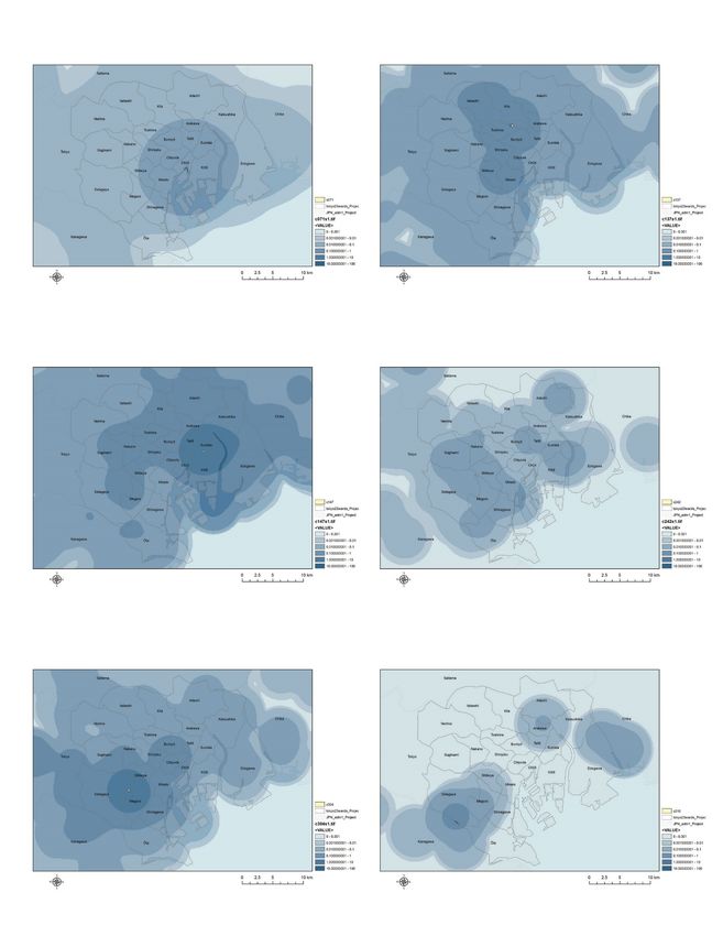
by a neighborhood park is 400 to 500m. In the case of district parks, the catchment area radius
would be 800 m to 1000 m (Ishida, 1987; Ishikawa, 2001).

   The park catchment area estimations and guidelines explained in the paragraphs above are
mostly based on normative criteria: neighborhood parks should be located within a five-minute
walking distance, for example. These guidelines also implicitly assume that people will use the
parks that they have closest access to. However, empirical evidence on actual park visit
behaviors and how far park visitors come from rarely exists, especially for neighborhood parks.
We can list up many other probable factors that may influence the park visit distance, such as job
location, transportation, physical environment of parks, beyond the simple distance between a
park and residential location. Due to the scarcity of related studies, we are yet to know how
different the assumed park catchment area and the actual park visit behavior are. Newly available
data that are able to show individual daily travels using georeferenced digital records open up the
possibility of understanding the actual park catchment area.

2.3. Usages of georeferenced location data and their application to the park catchment area
measurement
    Georeferenced data from various sources have been used to estimate human mobility and the
use of public facilities, including those related to parks (Evans-Cowley and Kitchen, 2011; Cao
et al, 2015; Rios and Munoz, 2017; Riggs and Gordon, 2018; Xiao et al., 2019). These real time
geocoded location data include sensor data, Internet of Things (IoT), and Point of Interests
(POIs) data (Fan et al, 2017; Rios and Munoz, 2017; Riggs and Gordon, 2018). For example,
Levin et al (2015) used data from the Flickr photo-sharing website as a proxy to identify which
areas people use for recreation.
    Also important are the data available from cell phones. Call Detailed Records (CDR) has
increasingly been recognized as a potential data source for new urban applications (Steenbruggen
et al, 2014). Using mobile base stations to identify the location of phone users, CDR data have
been applied to understand use patterns of urban facilities in complex environments. (Ratti et al,
2006; Xu et al, 2015). Florez et al (2017) also argued that CDR data from mobile phones are
novel resources for travel demand models.
    These geocoded location data are not without weaknesses including the spatial mismatch
between activities and records, inaccurate interpretation of location from the recording posts, and
bias toward particular types of application users. (Xu et al, 2015; Fan et al, 2017). Especially,
the CDR data, which rely on mobile base stations, are more prone to this precision issue as they
are the records of nearest or accessed base stations instead of the records of actual phone
locations (Xiao et al., 2019). In contrast, the Global Positioning System (GPS) records of mobile
phones are the records of the actual phone locations and thus greatly reduce the inaccuracy issue.

2.4. Measuring urban park catchment area with mobile data application
    In the use of mobile phone location data, it was not necessary to rely on the mobile base
station. Unlike Euclidean distance-based and network-distance based measures, this study
introduced a density-based approach to measure the UPCA. Density decay or a density gradient
is a conventional approach which has been used in urban economics (Louail et al, 2014). As

                                                 4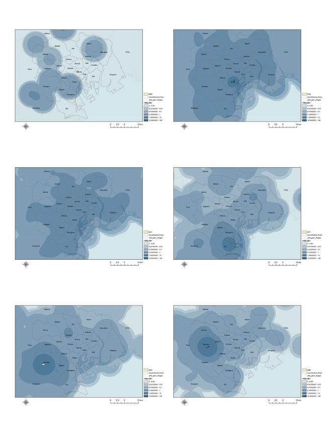
mentioned earlier, the actual usage of urban parks depends on many factors other than proximity
to the park such as safety, neighborhood social capital, function and facilities provided, size and
shape, terrain, and vegetation, among other things. (Madge, 1997; Pickett et al., 2016; Xiao et al,
2019). Under the assumption that people may use parks based on numerous criteria (not just the
parks that they have closest access to), multiple service areas can be applicable to measure
UPCA (Sorensen, 2002; Shin, 2004; Xiao et al., 2019). The benefit of using multiple service
areas is to reflect the frequency of park usage in addition to the physical proximity to parks.
Thus, we propose that multiple service radii should be used to understand park usage in contrast
to the conventional use of a single radius. In order to do so, we need to come up with density
gradient to capture the thresholds of the multiple service radii. Understanding the actual service
radius (radii) of UPCAs is critical for professionals involved in urban park planning, such as
policy makers, landscape designers, community advocates, and environmentalist, to have a better
grasp of the value of urban parks and come to agreement for decision making.

Figure 1. A model park plan of the first Five-year Plans for City Park Enhancement based on
Neighborhood Unit Planning principle. Source: Committee for the Publication of “Urban Parks
in Japan” 2005, page 69.

3. Data and Analytic Methods
3.1 Data collection

                                                 5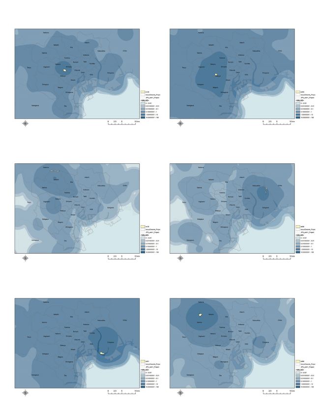
For a comprehensive understanding of park visitors in terms of both park size and seasonal
changes, we estimated and analyzed visitors of 30 urban parks, varying in size, in the central
Tokyo. The data collecting period includes four different months in 2011, representing each
season. The following sections explain the estimation process of park visitors and their
residential locations, and the sampling of parks and months.

Estimating park visitors and their residential locations
   We used the dataset called Konzatsu-Tokei ® Data from one of the predominant mobile
phone operators in Japan, with over 50 million subscribers. Konzatsu-Tokei ® Data refers to
people flows data aggregating individual location data sent from mobile phones under users'
consent, through applications such as “docomomap navi” service (map navi, local guide etc.)
provided by NTT DoCoMo, INC. Those data are processed collectively and statistically in order
to conceal the private information. The original location dataset is GPS data (latitude, longitude)
sent in about every minimum period of 5 minutes and does not include the information to specify
individual. (Akiyama, Horanont, & Shibasaki, 2013). Covering all areas of Japan, the dataset
includes all 365 days of the year 2011, from January 1 to December 31, and approximately 1.5
million cell phone IDs. This GPS point count is not the same as the total number of visitors of a
park although it is expected to be proportional to the actual volume of the visitors.
   To specify visitors of the sample parks, we introduced a two-step process. First, the park
boundary polygons and GPS points that were overlapping spatially were identified. Points within
the boundary of each sample park were assumed to be park visitors. Second, only the GPS points
that stayed longer than five minutes in a park were defined as a ‘visitor’. The accuracy error is in
general at a minimal level (within 15-30 meters in optimal conditions, that is to say without
obstructions of high-rise buildings) for those open air records. In the urban environment, the
error margin can be higher. We applied the five-minute criterion to exclude those who were
simply passing through the parks since those located closer to a transportation hub or crowded
streets are more likely to have a higher number of ‘passers-through’. This criterion was chosen as
a proxy to differentiate the purposes of travel / visit.
   We estimated the residential locations of the park visitors defined as above by tracing back
his/her daily movement. If the cell phone location of a visitor showed repeated stays at or around
the same point overnight throughout a year, the point is assumed as the residential location of the
visitor. The residential location detection criteria included (1) user is at residential location
between 8pm to 7am and (2) at least four days a week for more than half of the year. This
estimation enabled us to execute the following analyses on park visitor distribution.

3.2 Analytic Methods
Sampling time periods and parks
   As mentioned earlier, we picked four different months to sample all four seasons. More
precisely, we picked four weeks (28 days) for each season. The sampled weeks roughly overlap
with March, June, September, and December, see Table 1a.
   For the sampling of parks, we used the stratified random sampling based on the size of parks.
Japan’s Urban Park Law classifies urban parks into several categories and suggest recommended
size for each category. We chose five categories, roughly corresponding to the legal

                                                 6
classification and excluded the category for pocket parks, the smallest ones, see Table 1b. For
each of the five size categories, we selected six parks randomly. In sum, our park sample
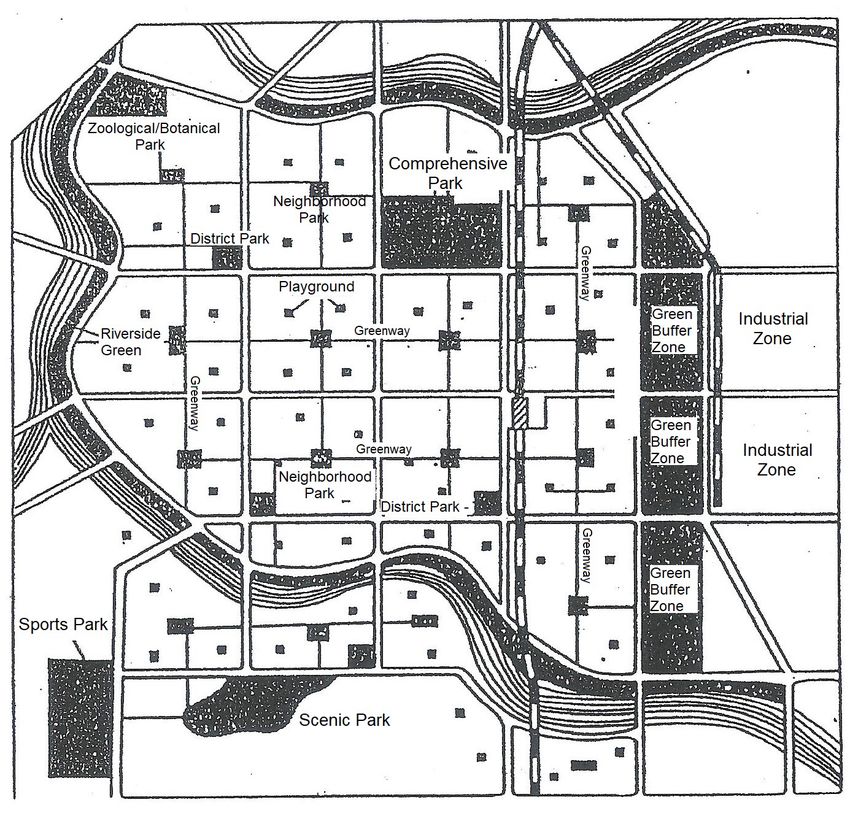
comprises a total of 30 parks and our analysis is based on visitors of the 30 parks during 16
weeks in 2011, see Figure 2.
Table 1a. Sampled periods
Season Spring Summer Autumn Winter
Period March 28 days June 28 days September 28 days December 28 days
(2011/03/05, SAT - (2011/06/04, SAT - (2011/09/03, SAT - (2011/12/03, SAT -
2011/04/01, FRI) 2011/07/01, FRI) 2011/09/30, FRI) 2011/12/30, FRI)
Table 1b. Summary of the parks sampled
Category Size Corresponding Total Number Sample Park List
Range Administrative of Parks in the
Category Size Range* Park ID Park Name (Location – Ku)
A1 (95) Kamezuga (Minato)
A2 (112) Kitakashiwagi (Shinjuku)
0.5 – 1 A3 (269) Magomenishi (Ota)
A City Block Park 217
ha A4 (278) Tamagawa Daishibashi (Ota)
A5 (371) Momozonogawa (Suginami)
A6 (392) Yabatagawaminami (Toshima)
B1 (70) Shin Tsukishima (Chuo)
B2 (109) Ochiai (Shijuku)
Neighborhood B3 (159) Yokoamicho (Sumida)
B 1 -3 ha 186
Park B4 (160) Mukojima Hyakkaen (Sumida)
B5 (252) Nakameguro (Meguro)
B6 (268) Higashichofu (Ota)
C1 (71) Ishikawajima (Chuo)
C2 (137) Rokugien (Bunkyo)
3 – 10 C3 (147) Kinshi (Sumida)
C District Park 103
ha C4 (242) Komaba (Meguro)
C5 (304) Setagaya (Setagaya)
C6 (310) Tamagawa Tamagawa (Setagaya)
D1 (63) Kokyo Higashigyoen (Chiyoda)
D2 (102) Shiba (Minato)
10 – 50 Comprehensive D3 (241) Shiokaze (Shinagawa)
D 51
ha Park D4 (271) Heiwano Mori (Ota)
D5 (343) Kinuta (Setagaya)
D6 (385) Wadabori (Suginami)
E1 (120) Shinjuku Gyoen (Shinjuku)
E2 (353) Yoyogi (Shibuya)
E3 (435) Arakawa Todabashi (Itabashi)
E 50 ha - National Park 10
E4 (606) Koiwa (Edogawa)
E5 (651) Kasai Linkai (Edogawa)
E6 (666) Hikarigaoka (Nerima)
*as of 2014, excluding ‘Marine Park’.
7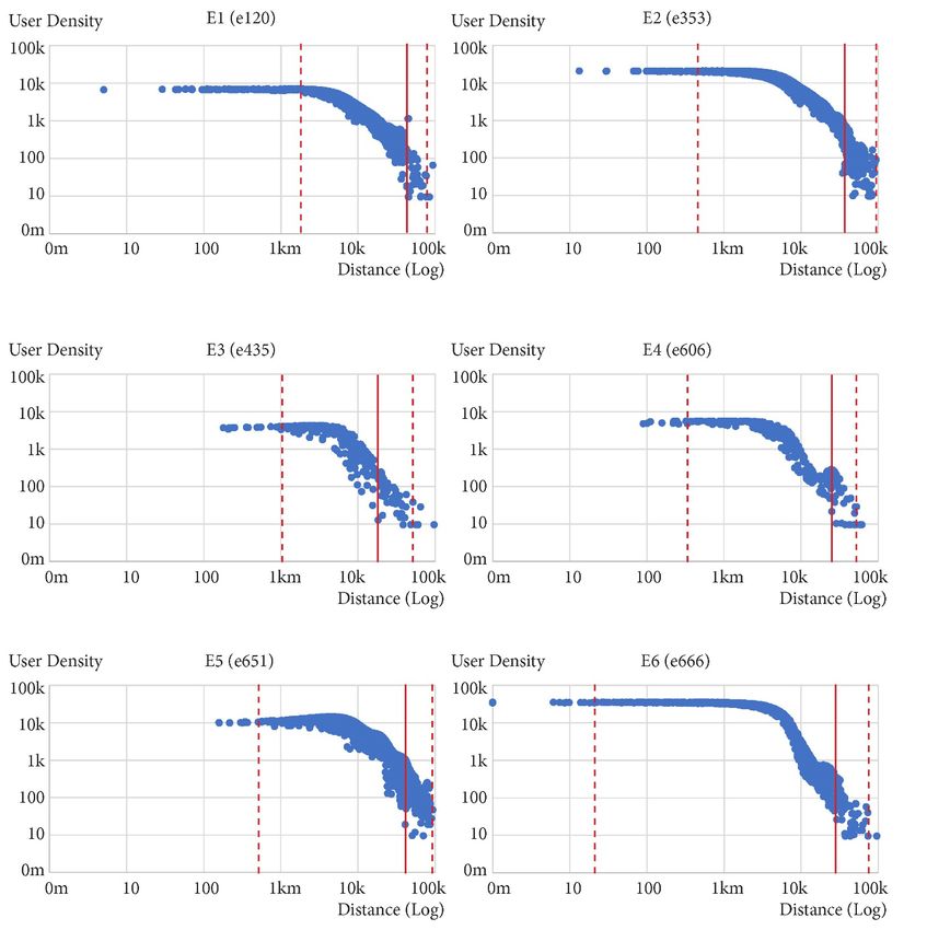
Figure 2. Location of parks.

Basic statistics, mapping, and density-based analysis
   To summarize the distance traveled for the park visits, the average, standard deviation,
median, and several percentile cut-offs were calculated based on the closest distance between the
estimated residential locations and the boundary of the parks using ArcGIS. We applied density-
distance mapping, density curve gradient, and density-distance decay function to measure
UPCA. (a) Density-distance maps were generated in ArcGIS, as the results of the spatial
interpolation of kernel density. Density distance gradients were used instead of distance-based
buffers to define urban park catchment areas. As such, the thresholds are the density or the
frequency of park visitors recorded in the sampling group. The results were exported to tables
and categorized by density thresholds to generate (b) Density curve gradient: A density curve
gradient was applied to identify the UPCA, using density cut-off thresholds (DTs). We
categorized park catchment areas using DTs of 0.001, 0.01, 0.1, 1, 10, and 100 users per km2.
We tried multiple search radiuses: When use radius higher than 5 km, the locational variation
starts to disappear. We then fixed the search radius as 5 km. In addition, 5 km is also roughly the
maximum distance to cover the shortest diameter of any of the 23 wards in Tokyo. We created 6
density groups, group 1 being the highest (over 100 park users) and group 6 being the lowest
(less than 0.001 park users) per km2. In order to captured the density variation of locations, we
measured (c) Density-distance decay function and “bandwidth”: The concept of a “bandwidth”
was used to measure density variation of locations that have the same distance to the center,

                                                 8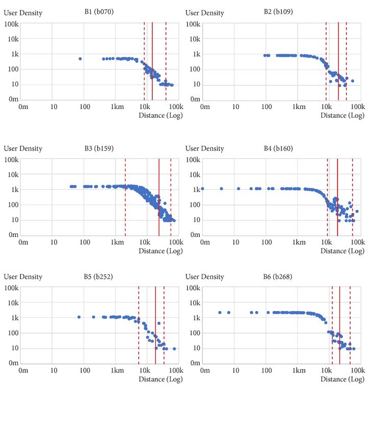
which in this case, were the selected urban parks. The higher the bandwidth, the greater the
variation. Together, the three analyses provide a comprehensive measure of UPCA.

4. Results
4. 1. Basic statistics
   Table 2 summarizes the results of the travel distance to sampled city block parks in Category
A. The study found that: (a) In general, the average travel distance to a city block park is much
longer than the median, suggesting that there were visitors originating from places further away
and hence increasing the average travel distance. (b) In five of the six cases, the median travel
distances fell within a rather reasonable range, from approximately 80m to 1.2km. At least half
of the visits originated from areas close to the city block parks. (c) Park A4, which had an
exceptionally high median travel distance, is a park adjacent to a large riverside park. One
explanation could be that there were many visitors originating from places further away to use
the large riverside open space regularly, such as sports club members. (d) There were also a
significant proportion of park visitors originating from places further away. They could be
workers, students, or other non-residents whose daytime jobs or schools are around the parks. (e)
Comparing the summary statistics including all repeat visitors and those excluding repeat
visitors, we find that the frequent visitors (repeats) originate from areas nearby the parks. This
shows that those repeat visitors are actual park users rather than those passing through to work.
The results of categories B, C, D and E are shown in Appendix 1. Considering the protection of
private information, comprehensive processing of the GPS data in this paper were performed in
ZENRIN Datacom Co., Ltd (ZDC) received the request of NTT DoCoMo and we were provided
only aggregated results.

Table 2. Summary of park travel distance (in meters).
               No. of    Average     SD        Median         10%        25%         75%       90%
               Obs*
                                          Including repeats
 A1(95)             75       9,153    15,837          463            4           4    10,772    32,690
 A2(112)            83       4,869    10,183          681           68          87     1,786    18,472
 A3(269)            62       4,014     7,950        1,160            9         244     1,160    11,558
 A4(278)           175      14,869    16,782       10,032           16         237    25,480    48,697
 A5(371)           275       6,355    10,703          239           10          36    10,101    20,886
 A6(392)           344      34,397   140,565           84            5          16     8,333    24,450
 Category A      1,014      17,280    83,434          716           10          34    10,338    27,129
                                          Excluding repeats
 A1(95)             26      13,111    20,533        4,239           40         463    15,906    33,392
 A2(112)            34       9,887    13,366        1,875           82         325    16,377    33,877
 A3(269)            18       4,925     7,907          998           20         188     4,308    20,300
 Magomenishi
 (Ota)
 A4(278)            56      13,527    16,362         2,608          84         390    26,968    39,232
 Tamagawa
 Daishibashi
 (Ota)
 A5(371)           156       8,546    12,250         3,550          20          92    12,794    24,917
 A6(392)           157      46,661   165,159         2,632          18          53    12,331    29,994
 Category A        447      22,779    99,894         2,458          21         105    14,255    29,994

                                                 9
Source: Konzatsu-Tokei ®, © ZDC.
* The number of visitors are based on the sampling data sets. The multiplier is 100+ based on the
total population. That is to say, for the smallest park categories, the visitors are in the range of
6,200 to 34,400 including multiple repeat visits. The numbers are much higher for other
categories.
4.2. Park catchment areas based on the density cut-off thresholds
The boundaries of the UPCAs were derived using six DTs. The spatial patterns of UPCAs
were observed across the five park size categories by area. The UPCAs are shown in Figure 3
(for Category A) and Appendix 2 (for Categories B, C, D, and E). We address (1) the area and
radius of the UPCA across different DTs; (2) the spatial patterns and shapes of the UPCA; and
(3) whether or not the UPCA is centered around the park.
For city block parks (Category A 0.5-1 ha), as shown in Figure 3, we observed circle shaped
UPCA at the highest DT at 10-100 park visitors per km2, for all parks. The shapes of the
catchments areas do not differ much from the conventional Euclidian distance derived
catchment. The radiuses of the circles are measured at 2.51km, 3.02km, 2.38km, 2.95km,
4.03km, and 4.12km, respectively, which is larger than most of the regulations (such as a 500m-
service radius) for a neighborhood park. At the 1-10 DT, UPCAs for Parks A1, A2, and A3 are
concentric circles of the 10-100 DT UPCAs. However, for parks A4, A5, and A6, the UPCAs of
the 1-10 DT are irregular shapes surrounding the 10-100 density threshold UPCA. In addition,
some of the UPCAs have two centers. For example, park A4 has a second catchment at the 1-10
threshold, appearing in the Arakawa-Sumita-Katsushika area, which is located diagonally across
the city.
The resultant catchment areas for neighborhood parks (Category B 1-3 ha) are shown in
Appendix 2. At the highest DT, the area of the UPCAs varied from 10.86km2 the smallest (B1)
to 143.0 7km2 (B3) the largest. Both circular-shaped (B1, B4, and B6) and irregular-shaped (B2,
B3, and B5) UPCAs were observed. Four of the parks’ UPCAs were centered and two were off-
centered (B3 and B5). Park B3 had irregularly-shaped UPCAs across all DTs. Park B1 has the
highest DT at 1-10 with a radius of 1.86km. Park B4 has two circular-shaped catchment areas at
the 10-100 DT. The larger one had a 3.75km radius centered around the park and the smaller one
had a 1.35km radius located 15km due west of the park. Park B6 has a circular-shaped catchment
with a radius of 3.81km at the 1-10 DT centered around the park.
For the district parks (Category C 3-10 ha), the UPCAs ranged from 1.33 km2 (C2) to 207.00
km2 (C1) (see Appendix 2) at the 10-100 DT. The circular shape catchment area was observed
only in park C5. The radius of the catchment area circle was 3.11km, centered around the park.
Park C1 had no UPCA at the 1-10 and 10-100 DT. At the 0.1-1 DT, Park C1 had a circular
catchment area. The results show that the frequency of park visitors to this park is lower than
other parks in this category. For this particular example, the study may not have enough data to
reveal the true catchment area of this park. Park C2 had a UPCA with a 650-meter radius at the
10-100 DT, centered around the perimeter of the park. At the 1-10 DT, the UPCA was irregular
in shape. Park C4 had multiple centers at the 0.1-1DT. Park C6 also has a circular catchment area
at the 1-10 density level with a radius of 1.92 km. The catchment area was not centered around
the park. At the 0.1-1 DT, there were multiple catchment areas.
10The comprehensive parks in Category D (10-50 ha) are shown in Appendix 2. The size of the
UPCAs at the highest respective DT ranged from 9.61 km2 (D1) to 715.96 km2 (D3). At the 10-
100 DT, we observed that four of the six parks had circular UPCAs: D2, D4, D5, and D6. Except
for park D4, the UPCAs were all centered around the park. Park D2 had a circular catchment
area at the 10-100 DT with a 1.76 km radius. There was a significant increase in the UPCAs
from 10-100 DT to 1-10 DT. This indicates that a further breakdown of the 1-10 DT can reveal
more useful information of the UPCA. Park D4 had a circular catchment area at the 10-100 DT
with a 2.81km radius. The UPCA was off-centered 1.62 km from the center of the park. The park
also has three separate catchments at the 1-10 DT, one around the park, one to the west, and the
third one to the northeast. The shape of the UPCA at the 0.1-1 DT became irregular. Park D5 had
a catchment roughly centered around the park at the 10-100 DT with a 3.75km radius. The
catchment areas at the 1-10 DT included two parts: one with a corrugated perimeter around the
park and the other was 13.72km away from the center of the park. Park D6 had a catchment area
centered around the park at the 10-100 DT with a 3.56 km radius. At the 1-10 DT, the catchment
was roughly centered around the park. However, the 0.1-1 DT catchment was irregularly shaped
with spokes radiating in different directions.
The parks in Category E (>50 ha) are shown in Appendix 2. The size of the UPCA at the 10-
100 DT varied from 2.83 km2 (e435) to 122.66 km2 (e353). None of the parks had a circular
catchment area at the 10-100 DT. However, three parks exhibited oval-shaped catchment areas:
E1, E2, and E4. In addition, two parks, E5 and E6, showed slightly deformed, circular service
areas. At the 10-100 DT, park E3 had a UPCA located 2km due south and with two catchment
areas. The larger one surrounded the park and the smaller one was 10 km away due south. Both
were oval shapes. At lower DTs, the shapes of UPCAs becomes irregular.
The important parameters (DT and its radius, shape, and location) used to delineating UPCA
are highly relevant to park planning: DT illustrates the density distribution of park users at
multiple levels. A higher DT shows more intensive usage of parks, which provides important
facts for maintenance and providing park user facilities. The radii of DTs can be used to compare
with existing park planning regulation. Shape and location of a UPCA are not only affected by
park size but also related to land use planning of the surrounding areas and transportation
accessibility. Next section further investigates the UPCA using density curve gradient.
11Figure 3. UPCA – Category A (0.5-1 ha).
Source: Konzatsu-Tokei ®, © ZDC.
124.3. Catchment area density curve gradient Using the conventional Euclidean distance and network distance catchment areas as baselines, the area density curve was expected to increase from high to low DT. The distance-based catchment is a function of A = πr2 (A is area and r is radius) and the network-based catchment is a function of buffer A = αsd2, (d is travel distance and s is speed). In both cases, it is a non-linear power function. However, what we observed using the DT method is a polynomial function. For the polynomial curve, two values are relevant in the UPCA derivation: the maximum value and the point of inflection. The point of inflection is where the distribution curve changes direction. In this study, the point of inflection indicates the DT at which most of the park user activities are captured. Moreover, if the maximum points are coinciding with the inflection points, the implication is that the DT that the inflection point is in should be subdivided and/or study areas should be extended. The inflection points can be observed in the catchment area density curve in Figure 4. The number of land parcels by DTs is summarized in Table 3. In category A, the largest number of land parcels for all parks were in the smallest DT (
City Scale           DT
 Park              10-100         1-10                0.1-1    0.01-0.1   0.001-0.01      < 0.001
 C2                    33       15,915               83,709     23,828         5,887       25,270
 C3                 6,350       47,252               74,726       6,117        1,843       18,354
 C4                     -            -               23,168     55,332        14,195       61,947
 C5                 3,990       24,725               62,357     32,620         6,417       24,533
 C6                     0        1,531               12,990     21,367         7,770      107,152
 D1                     -        1,040               27,976     14,578         4,190      103,026
 D2                 1,247       68,849               56,118       5,828        2,657       16,111
 D3                     -       58,281               67,402       5,313        2,418       17,396
 D4                 2,061       12,291               58,667     38,370         7,612       31,809
 D5                 4,801       18,482               70,799     25,790         5,288       25,650
 D6                 4,019        7,888               53,713     36,070         8,556       40,564
 E1                 2,550       61,903               59,616       4,788        1,873       20,080
 E2                13,859       99,306               14,733       3,840        1,890       17,182
 E3                   101       17,178               50,713     40,106         7,630       35,082
 E4                 1,816       16,036               64,703     35,665         5,608       26,982
 E5                 8,734      103,639               17,910       2,953        1,375       16,199
 E6                 9,196       25,308               75,768     19,725         3,033       17,780
Source: Konzatsu-Tokei ®, © ZDC.

4.4. Distance-Density decay function analysis
    The study observed that the catchment areas of the parks were positively associated with their
areas and revealed the applicable DT of the catchment areas. However, it is also important to
find out the activity patterns of park users and how they were spatially distributed in relevant to
the location of parks. Using the multi-scale catchment areas delineated earlier, the distance-
density relationship was analyzed using scatter plot charts, as shown in Figure 5 (for Category
A) and Appendix 3 (for Categories B, C, D, and E).
    If the distance-density decay function holds, it means the further away from the park, the less
visitors come to the park. The other important variable in the distance-density function of UPCA
is bandwidth. As mentioned earlier, bandwidth captured the variation in density locations. With
the exception of park A2, most city block parks (Category A) showed an inverse relationship
between distance and density within a 100 m radius. In the case of park A2, there were too few
observations to draw a conclusion. Within 1 km, all parks complied with the distance-density
decay rule. Between 1 km and 5 km, distance-density decay function was only observed in parks
A5 and A6. Between 5 km and 10 km, the decay function was also observed in parks A5 and A6,
however, the rate of decay was higher. After 10 km, no decay function was observed. The
bandwidth is shown in Appendix 4.
    In the neighborhood parks (Category B), parks B3, B4, and B6 exhibited the density-distance
decay function within a 100 m radius from the perimeter of the parks. Between 1km and 5km
and between 5 km and 10 km, all the neighborhood parks, with the exception of park B1,
exhibited the decay function. From the analysis, park B3 deserves closer investigation because
the variation of density distribution at the same distance was large. This broader bandwidth
implies higher variation of density location. In the district parks (Category C), C2 and C3 had

                                                14
broader bandwidths of density distributions for all distances observed. Parks C1 and C4 followed
the density distance decay function until a radius of 5 km, then the bandwidth of density began to
increase. In the comprehensive parks (Category D), all but D1 showed broader bandwidths of
density. Park D1 did not have sufficient points that were valid (not that there are few visitors, on
the contrary, there are more than 1,000 visit observed). In the national parks in Category E, all
exhibited higher bandwidths of density distribution. For larger parks, not only should the study
extend beyond the city scale, the higher density threshold (10-100) should also be subdivided to
observe more nuanced variations.
15Figure 4. UPCA density-area curves by surface area categories: normalized into six density
thresholds. Each line represents a park. The x-axis is density of park visitors. The y-axis is area
measured in hectares, representing the theoretical catchment area. Source: Konzatsu-Tokei ®, ©
ZDC.
Figure 5. Park user density – distance function. Source: Konzatsu-Tokei ®, © ZDC.
165. Discussion
5.1. Delineating the UPCA using the density thresholds
One of the contributions of this paper was to delineate a UPCA based on actual park user
activity. The data required was GPS-enabled mobile phone location data. The Euclidean distance
derived UPCAs were based on locations of the facilities, which rarely change; the network
distance derived UPCAs were based on the infrastructure network, which change overtime with
financial investment cycles and varies due to services provided; the mobile phone location
derived UPCA were delineated based on actual park user activity, which is inherently dynamic
because of their travel patterns.
For smaller city block parks in category A, the average UPCA radius derived was 3.17 km,
which is larger than defined by most of the existing planning regulations. For example, a 500 m
service radius for a neighborhood park. If the density threshold was increased, from 10 to 50
visitors per km2, for example, the resultant radius would be smaller. A DT corresponding to a
500 m-radius catchment circle could be derived. However, the results showed that even for the
smallest park category, a higher percentage of visitors were from outside of the 500 m radius.
The appropriate DTs used to derive the UPCAs, as mentioned earlier, should follow the
maximum and inflection points of the density area curves. Depending on the number of DTs
applied, the resultant UPCA would have multiple instead of singular centers.
5.2. Interpreting UPCA use spatial parameters
In both the city block and neighborhood parks (Categories A and B), the highest DT
catchments encircled the corresponding parks. The explanation is that for smaller parks between
0.5 and 3 hectares, the proximity to parks is strong correlated with the usage of parks. For district
and comprehensive parks (Categories C and D), there was considerable variation in the area and
shape of the UPCA. This suggests that after the park size reached over 3 hectares, the usage of
parks depends on many other factors (such as location, accessibility, function, and facilities
provided) other than proximity. For example, park C6 exhibited similar catchment areas as the
city block parks in category A, with concentric circles around the park. This anomaly suggests
that park size is not the determinant factors. For parks C2, C3, and C5, the highest density
threshold reached 10-100 DT and at the 1-10 DT, they exhibited irregular shapes instead of
circles. Park D1 shows similar patterns of UPCA as those in city block parks. This shows even
comprehensive parks can have a catchment area attracts only people from close by. On the other
hand, park D2 has the largest number of land parcels in the 1-10 DT. It suggested that the
delineated UPCA cannot effectively differentiate across park user activities.
The shape of the catchment area did not necessarily become more irregular as the area
increased. For example, there were more circular UPCA in the comprehensive parks than the
district parks. In addition, the shape of the park can affect the shape and area of the parks. For
example, parks E3 and E4 are linear because they are riverside waterfront parks. The nature of
the park may contain systematic patterns reflected in the catchment areas.
5.3. Relating UPCA to land use and infrastructure
Area of DT, shape, and location are three important parameters defining an UPCA. While
conventional park planning mainly relies on park surface area and facilities provided, the
17combination of area of DT, shape, and location of UPCAs can provide additional information to
understand park usage. In general, the UPCA is positively correlated with the park areas. We can
identify anomaly when this is not the case. For example, when a large park has a relatively small
catchment area. Moreover, the shape of the UPCA can indicate travel mode and activities of park
usage. For example, an irregular shaped UPCA could be affected by transit lines that people used
to visit park. Another example is that some of the UPCAs’ geometric centers do not match the
location of the park. This can occur in riverfront parks where the main activity is the gathering of
sports club members who travel (drive) from far distance. While most of the UPCA with the
highest DT are circular, oval-shaped UPCAs began to emerge in the district parks (Category C).
For example, park C3, at the 10-100 DT was an oval shape with cross diameters of 4.25 km and
4.9 km respectively. Furthermore, the center of the oval-shaped UPCA was over 500 m away
from the park. We suggest that the shape of the UPCA can be a function of external
characteristics such as land use and infrastructure of the broader city beyond the study areas. We
also suggest that the provision of facilities, vegetation, and amenities in the parks and the
proximity to other parks can be important determinants of the UPCA. In this paper, we didn’t
investigate these conditions.
5.4. Limitations
While the application of mobile phone data improved our understanding of the UPCA, the
limitations that can be addressed in future studies include: First, more investigations into the
facilities provided in and around the parks, such as land use and park function. Second, the
conclusion can be strengthened if more parks were included. We can extend study to duration of
stay by park visitors; group or individual activities; and daily, weekly, and seasonal variations.
Third, the office staff who visit parks near their companies but far away from residential location
were not excluded. In this study, we want to include all visits, not just “directly from residential
location to park” type. We didn’t include people who visited parks near their secondary
residential locations as well as moving, traveling, and intro-company job relocations/transfers
(Tenkin) during the study period in our analysis as they only represent a small percent of the
samples. Last, the selection of radius is arbitrary: as the search radius become smaller, density,
shape, and size of the catchment areas can also change. All of the above-mentioned can affect the
actual catchment area, together with social capital cultivation, cultural adaptation, weather
variations.
6. Conclusions
In this paper, the UPCA was delineated using GMD in the Tokyo metropolitan area. Deriving
the UPCA is important as it can affect current park planning practice in the following ways: (1)
Demonstrate individual travel distances to parks; and (2) Account for diversity in park visitors of
different park surface areas. Through the use of density-distance mapping, density curve
gradient, and density-distance analysis, this study found that (a) The UPCAs were positively
correlated with the park areas, albeit with variations within each park category; (b) Almost all the
parks, regardless of its size and function, had the highest user density right around the vicinity.
This is exemplified by the density distance function closely follow a decay trend line within 1-2
18km radius of the park. However, across all the parks, beyond the 5-10 km radius, the density-
distance decay function was not observed.
References
Ahas, R., Silm, S., Järv, O., Saluveer, E., & Tiru, M. (2010). Using mobile positioning data to model
locations meaningful to users of mobile phones. Journal of urban technology, 17, 3–27.
Akiyama, Y., Horanont, T., & Shibasaki, R. (2013). Time-series Analysis of Visitors in Commercial
Areas Using Mass Person Trip Data (大規模人流データを用いた商業地域における来訪者数の時
系列分析). Paper presented at the GIS Association of Japan: 22nd Annual Conference, Tokyo, Japan.
Bedimo-Rung, A. L., Mowen, A. J., & Cohen, D. A. (2005). The significance of parks to physical activity
and public health: A conceptual model. American Journal of Preventive Medicine, 28, 159–168.
Chang, H.-S., & Liao, C.-H. (2011). Exploring an integrated method for measuring the relative spatial
equity in public facilities in the context of urban parks. Cities, 28, 361–371.
Committee for the Publication of “Urban Parks in Japan” (Ed.) (2005). Urban Parks in Japan: The
History of Construction and Maintenance (日本の都市公園 : その整備の歴史). Tokyo, Japan:
Intarakushon/Kankyo Ryokuka Shimbun.
Dai, D. (2011). Racial/ethnic and socioeconomic disparities in urban green space accessibility: Where to
intervene? Landscape and Urban Planning, 102, 234–244.
Fan, P., Xu, L., Yue, W., & Chen, J. (2017). Accessibility of public urban green space in an urban
periphery: The case of Shanghai. Landscape and Urban Planning, 165, 177–192.
Florez, M, Jiang, S. Li, R. Mojica, C., Transmilenior, S., Rios, R., Gonzalez, M. (2017) Measuring the
impact of economic well-being in commuting networks–A case study of Bogota, Colombia.
Proceedings of the Transportation Research Board 96th Annual Meeting. 1-19.
Giles-Corti, B., Broomhall, M. H., Knuiman, M., Collins, C., Douglas, K., Ng, K., Donovan, R. J. (2005).
Increasing walking: How important is distance to, attractiveness, and size of public open space?
American Journal of Preventive Medicine, 28(2), 169–176.
https://doi.org/10.1016/j.amepre.2004.10.018.
Gobster, P. H. (2002). Managing urban parks for a racially and ethnically diverse clientele. Leisure
Sciences, 24, 143–159.
Grahn, P. and Stigsdotter, U. (2003) Landscape planning and stress. Urban Forestry & Urban Greening,
2(1), 1-18.
Guan, C., Srinivasan, S. and Nielsen, P. (2019) Does neighborhood form influence low-carbon
transportation in China? Transportation Research Part D: Transport and Environment, 67, 406-420.
Ishida, Y. (1987). One Hundred Years of Japanese Modern Urban Planning (日本近代都市計画の百
年). Tokyo, Japan: Jichitaikenkyusha.
Ishikawa, K. (2001). Cities and Green Space (都市と緑地:新しい都市環境の創造に向けて). Tokyo,
Japan: Iwanamishoten.
La Rosa, D. (2014) Accessibility to greenspaces: GIS based indicators for sustainable planning in a dense
urban context. Ecological Indicators 42: 122–134.
Lancaster, R. A. (1983). Recreation, park and open space standards and guidelines. Recreation, Park and
Open Space Standards and Guidelines, 1(4), 141–168.
Liang H and Zhang Q (2018) Assessing the public transport service to urban parks on the basis of spatial
accessibility for citizens in the compact megacity of Shanghai, China. Urban Studies 55 (9), 1983-
1999.
Louail, T. et al. (2014) From mobile phone data to the spatial structure of cities. Scientific Reports 4,
5276.
Madge, C. (1997). Public parks and the geography of fear. Tijdschrift voor economische en sociale
geografie, 88, 237–250.
19Marcus, C. and Francis M. (1998). People Places: Design Guidelines for Urban Open Space. New York:
Wiley.
Perry, C. (1929) The Neighbourhood Unit. Reprinted Routledge/Thoemmes, London, 1998, 25-44.
Pickett, S. T., Cadenasso, M. L., Childers, D. L., McDonnell, M. J., & Zhou, W. (2016). Evolution and
future of urban ecological science: Ecology in, of, and for the city. Ecosystem Health and
Sustainability, 2, e01229.
Ratti, C., Frenchman, D., Pulselli, R. M., & Williams, S. (2006). Mobile landscapes: Using location data
from cell phones for urban analysis. Environment and Planning. B, Planning & Design, 33(5), 727–
748.
Ríos, S. A., & Muñoz, R. (2017). Land use detection with cell phone data using topic models: Case
Santiago, Chile. Computers, Environment and Urban Systems, 61, 39–48.
Reyes, M, Paez A., and Morency, C. (2014) Walking accessibility to urban parks by children: A case
study of Montreal. Landscape and Urban Planning 125: 38–47.
Shin, Y. (2004). Urban Park Policy Development History (都市公園政策形成史: 協働型社会における
緑とオープ ンスペースの原点). Tokyo, Japan: Hosei Daigaku Shuppankyoku.
Sorensen, A. (2002). The Making of Urban Japan: Cities and Planning from Edo to the Twenty-first
Century. Abingdon, UK: Routledge
Stock K (2018) Mining location from social media: A systematic review. Computers, Environment and
Urban Systems, 71, 209-240.
Van Herzele, A., & de Vries, S. (2011). Linking green space to health: A comparative study of two urban
neighbourhoods in Ghent, Belgium. Population and Environment, 34(2), 171–193.
https://doi.org/10.1007/s11111-011-0153-1.
Wolch, J. R., Byrne, J., & Newell, J. P. (2014). Urban green space, public health, and environmental
justice: The challenge of making cities ‘just green enough’. Landscape and Urban Planning, 125,
234–244.
Woolley, H. (2003) Urban Open Spaces. Spon Press, London.
Xiao Y, Wang D and Fang J (2019) Exploring the disparities in park access through mobile phone data:
Evidence from Shanghai, China. Landscape and Urban Planning, 181, 80-91.
Xu, Y., Shaw, S.-L., Zhao, Z., Yin, L., Fang, Z., & Li, Q. (2015). Understanding aggregate human
mobility patterns using passive mobile phone location data: A home-based approach. Transportation,
42(4), 625–646.
Xu, Z., Gao, X., Wang, Z. & Fan, J. (2019) Big data-based evaluation of urban parks: A Chinese case
study. Sustainability, 11, 2124-2125.
Yuan, Y., Raubal, M., & Liu, Y. (2012). Correlating mobile phone usage and travel behavior – A case
study of Harbin, China. Computers, Environment and Urban Systems, 36(2), 118–130.
Zhai Y, Wu H, Fan H, Wang D (2018) Using mobile signaling data to exam urban park service radius in
Shanghai: methods and limitations. Computers, Environment and Urban Systems, 71, 27-40.
Zhang S. and Zhou W. (2018) Recreational visits to urban parks and factors affecting park visits:
Evidence from geotagged social media data. Landscape and Urban Planning, 180, 27-35.
Zhao D and Stefanakis E (2018) Mining massive taxi trajectories for rapid fastest path planning in
dynamic multi-level landmark network. Computers, Environment and Urban Systems, 72, 221-231.
20Appendix 1. Basic statistics on travel distance.
No. of
Average SD Median 10% 25% 75% 90%
Obs
Including duplicates
B1(70) 125 11,847 12,710 8,403 676 1,922 17,360 29,811
B2(109) 151 8,080 11,069 2,370 347 814 10,761 24,521
B3(159) 554 13,204 11,874 9,106 1,146 4,958 19,090 30,458
B4(160) 264 15,623 17,224 10,857 4 587 24,181 44,149
B5(252) 228 9,801 10,755 3,455 418 1,150 20,790 23,597
B6(268) 305 4,880 8,592 1,417 7 358 4,093 13,283
Category B 1,627 10,979 12,755 6,291 204 1,289 16,346 27,479
Excluding duplicates
B1(70) 71 15,738 14,533 12,484 1,464 3,387 21,377 37,936
B2(109) 84 9,661 11,020 6,255 353 1,090 14,044 26,483
B3(159) 221 14,608 14,017 10,163 659 3,587 22,490 35,426
B4(160)
121 14,984 16,800 9,105 432 1,860 20,637 37,169
Mukojima Hyakkaen (Sumida)
B5(252) 54 10,814 13,526 5,341 724 1,370 17,522 27,842
B6(268) 117 7,146 11,108 2,481 316 754 6,199 23,055
Category
668 12,561 14,101 7,754 456 1,814 18,128 31,722
B
No. of
Average SD Median 10% 25% 75% 90%
Obs
Including duplicates
C1(71) 128 14,279 14,334 10,607 61 94 31,932 33,404
C2(137) 1,103 12,479 12,133 8,448 368 3,085 17,928 30,779
C3(147) 3,762 12,554 15,663 6,900 342 1,640 17,082 32,686
C4(242) 99 13,881 13,605 8,399 228 3,251 18,926 40,146
C5(304) 1,663 7,767 11,295 3,066 218 729 10,637 18,762
C6(310) 86 12,541 13,842 3,223 320 1,068 27,620 33,165
Category C 6,841 11,430 14,242 6,511 258 1,210 16,155 30,779
Excluding duplicates
C1(71) 52 11,785 12,901 6,140 65 381 19,834 32,242
21No. of
Average SD Median 10% 25% 75% 90%
Obs
Ishikawajima (Chuo)
C2(137) 392 13,701 12,467 10,844 718 3,570 18,876 31,577
C3(147)
1,867 11,453 13,041 6,638 812 2,114 16,590 29,628
Kinshi (Sumida)
C4(242)
53 10,986 11,464 7,655 541 2,057 15,686 26,865
Komaba (Meguro)
C5(304) 497 10,882 14,498 5,194 517 1,179 14,565 30,201
C6(310) 27 10,086 11,957 3,380 264 1,068 21,433 29,611
Category
2,888 11,645 13,206 6,895 699 1,993 16,960 30,244
C
No. of
Average SD Median 10% 25% 75% 90%
Obs
Including duplicates
D1(63) 1,068 353,017 306,386 345,046 16,457 51,731 516,782 887,836
D2(102) 2,892 17,274 13,746 14,233 1,657 7,568 24,611 35,692
D3(241) 1,996 20,247 12,592 17,911 5,965 10,767 28,342 36,911
D4(271) 1,138 10,508 11,944 4,132 212 1,638 17,906 29,214
D5(343) 2,003 6,318 8,917 2,566 82 576 8,023 19,677
D6(385) 1,121 4,720 9,641 1,228 13 273 4,703 13,648
Category D 10,218 48,669 144,134 11,457 349 2,596 25,265 47,267
Excluding duplicates
D1(63)
Kokyo Higashigyoen 502 255,507 272,665 122,095 15,999 36,408 401,453 749,825
(Chiyoda)
D2(102) 1,868 18,764 14,480 14,993 3,411 8,222 27,261 37,263
D3(241)
768 20,451 13,336 17,407 5,783 10,664 28,642 38,906
Shiokaze (Shinagawa)
D4(271) 371 10,695 12,256 4,620 413 1,784 17,669 29,356
22No. of
Average SD Median 10% 25% 75% 90%
Obs
D5(343) 598 9,210 10,390 5,095 659 1,654 13,549 23,086
D6(385) 377 7,426 11,166 2,872 342 949 9,465 20,360
Category
4,484 42,662 119,152 14,149 1,411 5,641 28,831 47,974
D
No. of
Average SD Median 10% 25% 75% 90%
Obs
Including duplicates
E1(120) 3,448 51,235 149,190 15,224 2,538 6,947 30,718 48,326
E2(353) 10,316 46,399 126,746 13,574 2,149 5,982 28,494 67,326
E3(435) 968 33,630 123,266 5,313 1,714 2,373 13,265 28,053
E4(606) 1,071 18,692 73,110 3,653 693 1,358 8,674 25,923
E5(651) 9,786 46,991 109,013 20,643 4,682 11,622 36,925 77,335
E6(666) 5,439 23,840 109,833 1,879 169 608 7,341 23,845
Category E 31,028 41,814 120,149 13,368 915 4,006 27,520 56,679
Excluding duplicates
E1(120)
1,224 56,361 164,886 14,388 2,631 6,495 28,669 66,480
Shinjuku Gyoen (Shinjuku)
E2(353) 4,129 55,772 140,612 15,401 2,900 7,213 31,592 95,186
E3(435) 328 33,784 114,109 7,187 1,710 2,901 17,110 35,396
E4(606) 337 28,537 98,526 6,114 901 2,613 18,807 31,658
E5(651) 3,556 52,389 121,291 21,092 4,663 11,672 37,740 84,271
E6(666) 1,585 30,426 124,026 3,388 403 1,126 11,910 28,357
Category
11,159 49,689 133,918 15,122 1,828 5,738 30,059 76,308
E
Source: Konzatsu-Tokei ®, © ZDC.
23Appendix 2. UPCA–Categories B, C, D, and E.
UPCA– Category B (1-3 ha).
24UPCA– Category C (3-10 ha).
25UPCA– Category D (10-50 ha).
26UPCA–Category E (50 ha and above).
Source: Konzatsu-Tokei ®, © ZDC.
27Appendix 3. Park user density – distance function.
2829
30
Source: Konzatsu-Tokei ®, © ZDC.

                                   31
Appendix 4. Measure of bandwidth in the density-distance function chart.
In this box plot, x axis is the log-distance and the y axis is user density categorized in 0.1 log-
distance intervals. The highest variance is 1.42 happened at log-distance 4.5 and the emergence
of bandwidth happened at log-distance 3.8 end at 4.7.
32You can also read