Total Cluster: A person agnostic clustering method for broadcast videos
←
→
Page content transcription
If your browser does not render page correctly, please read the page content below
Total Cluster: A person agnostic clustering method for
broadcast videos
Makarand Tapaswi1 , Omkar M. Parkhi2 , Esa Rahtu3
Eric Sommerlade2 , Rainer Stiefelhagen1 , Andrew Zisserman2
1
Computer Vision for Human Computer Interaction, Karlsruhe Institute of Technology, Germany
2
Visual Geometry Group, Department of Engineering Science, University of Oxford, UK
3
Center for Machine Vision Research, University of Oulu, Finland
tapaswi@kit.edu, omkar@robots.ox.ac.uk, erahtu@ee.oulu.fi
eric@robots.ox.ac.uk, rainer.stiefelhagen@kit.edu, az@robots.ox.ac.uk
ABSTRACT
The goal of this paper is unsupervised face clustering in … …
edited video material – where face tracks arising from differ-
ent people are assigned to separate clusters, with one cluster
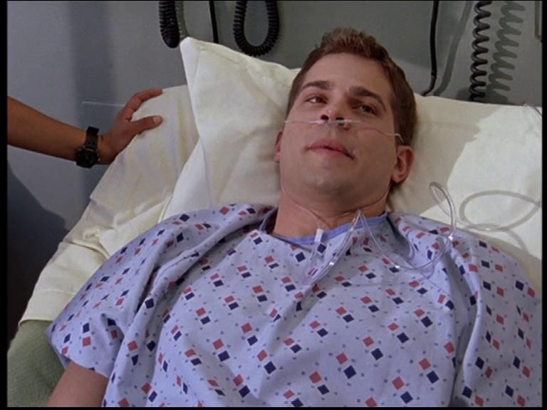
for each person. In particular we explore the extent to which Tracks and cannot-links within shots of a scene
faces can be clustered automatically without making an er-
ror. This is a very challenging problem given the variation
in pose, lighting and expressions that can occur, and the
similarities between different people.
The novelty we bring is three fold: first, we show that a
form of weak supervision is available from the editing struc-
ture of the material – the shots, threads and scenes that Tracks and cannot-links within a shot thread pattern
are standard in edited video; second, we show that by first
clustering within scenes the number of face tracks can be
significantly reduced with almost no errors; third, we pro-
pose an extension of the clustering method to entire episodes
using exemplar SVMs based on the negative training data
automatically harvested from the editing structure.
Tracks within a scene
The method is demonstrated on multiple episodes from
two very different TV series, Scrubs and Buffy. For both Figure 1: Overview of the video-editing structure of a
series it is shown that we move towards our goal, and also TV series episode. Face tracks are shown for single shots
outperform a number of baselines from previous works. of a scene (top row), in a threading pattern (middle row)
and in a scene (bottom row). Face tracks with the same
Keywords color denote the same person. Must-not links between
Face track clustering, TV shows, Video-editing structure tracks are denoted by red edges. (Best viewed in colour)
1. INTRODUCTION
Television broadcasting has seen a paradigm shift in the actor appears. Enabling such search services requires anno-
last decade as the internet has become an increasingly im- tating the video content, and this is the goal towards which
portant distribution channel. Delivery platforms, such as we work here.
the BBC’s iPlayer, and distributors and portals like Netflix, Our objective is to automatically cluster face tracks
Amazon Instant Video, Hulu, and Youtube, have millions of throughout a broadcast according to identity, i.e. to as-
users every day. These new platforms include search tools sociate all the face tracks belonging to the same person.
for the video material based on the video title and metadata If successful, then annotating the video content for all
– however, for the most part it is not possible to search di- actors simply requires attaching a label (either manually or
rectly on the video content, e.g. find clips where a certain automatically) for each cluster. There are many previous
works that consider automatic face labelling in broadcast
videos [2, 6, 5, 7, 9, 10, 25, 27, 29] but all of these require
Permission to make digital or hard copies of all or part of this work for
personal or classroom use is granted without fee provided that copies are supervision in some form, typically subtitles and transcripts.
not made or distributed for profit or commercial advantage and that copies Our approach of unsupervised clustering is complementary
bear this notice and the full citation on the first page. To copy otherwise, or to these and the transcript supervision can be applied to
republish, to post on servers or to redistribute to lists, requires prior specific automatically label the clusters. Furthermore, our clus-
permission and/or a fee. tering is also applicable in cases where transcripts are not
ICVGIP ’14, December 14-18, 2014, Bangalore, India available, e.g. for older or archive material. Here, manual
Copyright is held by the authors. Publication rights licensed to ACM.
ACM 978-1-4503-3061-9/14/12 ...$15.00 effort can be greatly reduced compared to labelling all face
http://dx.doi.org/10.1145/2683483.2683490. tracks individually.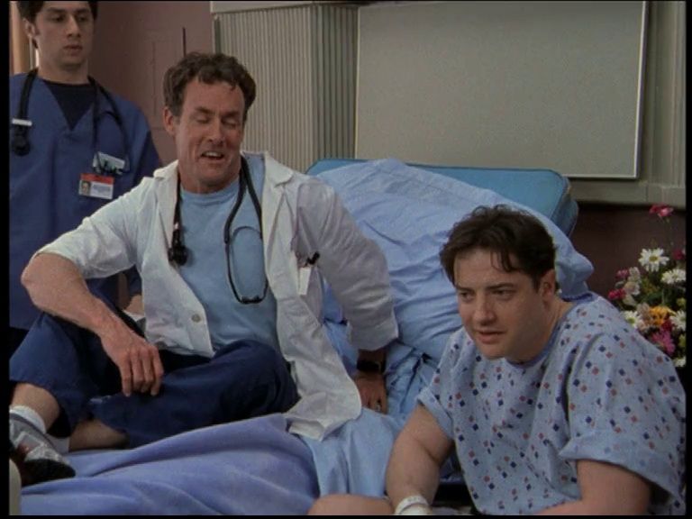
The novelty we bring is to take account of the editing          “ABAB ” shot structuring; the “over-the-shoulder” shot for
structure of the video (Sect. 3) when considering candidate        dialogue exchange between two characters; the 180 degree
face tracks to cluster. These cues have not been used in           rule, etc. In this section, we briefly describe a few typi-
previous works (Sect. 2 on related work). In particular we         cal structures used in the video editing process – namely
show that: (i) the thread structure can be used both to de-        shots, threads and scenes. Figure 1 provides examples of
termine must-not and do links between face tracks; (ii) clus-      face tracks seen in shots, threads and scenes of an episode.
tering first within scenes allows pure clusters to be obtained
whilst significantly reducing the number of unassigned face        3.1   Shots
tracks; and (iii) these clusters can subsequently form strong        A shot refers to a group of consecutive frames filmed from
classifiers for between scene clustering.                          the same camera. In this paper, we segment shots by detect-
   In addition, we make two technical contributions: (i) we        ing their boundaries using a normalized version of the Dis-
improve on the standard frontal face detectors used in face        placed Frame Difference (DFD) [33]. The DFD captures the
clustering by also including profile detections and upper-         difference between consecutive motion compensated frames
body detections; and (ii) we make use of the recently in-          and produces peaks at shot boundaries as the optical flow
troduced Fisher Vector based face track representation with        cannot compensate the sudden change in camera.
discriminative dimensionality reduction [19] (Sect. 7).              In our case, a shot also limits the temporal extent of any
   As will be seen (Sect. 6), we are able to substantially re-     face track. In other words, all detections in any face track
duce the number of face tracks that need to be labelled.           must belong to the same shot. In previous work, e.g. [3,
Though we do not reach the goal of one cluster per actor,          32], temporal co-occurrence of two face tracks in a shot has
the proposed method obtains better clustering performance          been used to form examples of track pairs that must depict
compared to a number of baselines based on previous ap-            different characters. We will also use this as one approach
proaches.                                                          for producing cannot-link constraints and negative training
                                                                   examples.
2.   RELATED WORK
   In this section, we review previous work on unsupervised        3.2   Threads
face track clustering.
                                                                      A thread is a sequence of shots, obtained from the same
   One approach is to cast face clustering as a pure data clus-
                                                                   camera angle and located in a short temporal window (see
tering problem and attempt to solve it using general purpose
                                                                   Fig. 2). Typically threads form patterns like “ABAB ” where
algorithms. For instance, a hierarchical bottom up agglom-
                                                                   the story is presented using alternating shots from two dif-
erative clustering was applied in [3], [14], and [22]. Cinbis et
                                                                   ferent cameras that form threads A and B. Such patterns
al . [3] utilise a special distance metric that is learned us-
                                                                   work well with the previously mentioned “over-the-shoulder”
ing automatically obtained positive and negative face pairs.
                                                                   shots as they depict dialogues between characters standing
Similarly, Khoury et al .[14] learn a metric based on a com-
                                                                   opposing each other. Note that A and B in the “ABAB ”
bination of appearance cues and Gaussian Mixture Models.
                                                                   denote threads (cameras) and not two different people. It is
   A second approach is to construct a graphical model of
                                                                   not uncommon to have more than one visible character in
the face detections or tracks and formulate the clustering
                                                                   each thread.
as an optimization problem on the graph. As in [3], con-
                                                                      A threading pattern can also be more complex and involve
straints between nodes of a graph are obtained by assuming
                                                                   more than two cameras (see Fig. 2). For example, during
that all detections in one face track belong to the same actor
                                                                   a dialogue between two people, two different cameras can
and that one person cannot appear twice in the same frame.
                                                                   provide close-up face shots of the speakers, while a third one
Wu et al .[31, 32] use a Hidden Markov Random Field model
                                                                   gives an overview of the setting (a group shot) in which they
to improve face tracking, by first detecting faces, creating
                                                                   are conversing. Such a setup can form threading patterns
small “tracklets” and then joining them using a constrained
                                                                   such as “ABCACBCA” where A and B are as above and C
clustering method, with [32] extending [31] by clustering
                                                                   is the thread obtained from the third view.
across shots. However, both [31, 32] require the number
                                                                      While many shots (and thus tracks) are part of a threading
of output clusters K to be specified, and this information is
                                                                   pattern, there are others which do not form any thread. An
not available in our case.
                                                                   example of a shot which does not belong to a thread is a
   A third approach is to explicitly utilise the video struc-
                                                                   long take – a shot that pans across a large part of the set
ture in clustering. For instance, Ramanan et al . [21] use a
                                                                   and follows the actors on screen.
notion of shots and scenes and first perform agglomerative
                                                                      An analysis of our Scrubs and Buffy data sets (cf . Tab. 1
clustering in each shot, then in each scene, and finally in
                                                                   and 2 respectively) shows that about 60-70% of shots belong
the episode. At each level, they apply a different feature
                                                                   to a thread and correspondingly more than 68% of all face
weighting (on faces, hair and clothing).
                                                                   tracks belong to a shot which is in a threading pattern.
   We also note that others have used video editing structure,
                                                                      We detect shot threads using a method proposed in [28]
such as threads, for various tasks [4, 6], e.g. for detecting
                                                                   that computes SIFT matches between the last frame of a
continuity errors [20] or generating story graphs [28], but as
                                                                   shot and the first frame of F subsequent shots. The threads
far as we know we are the first to use the editing structure
                                                                   are used to generate both highly confident must-link (pos-
in this manner to provide supervision for unsupervised face
                                                                   itive) pairs and cannot-link (negative) pairs between face
clustering.
                                                                   tracks.

3.   VIDEO STRUCTURE                                               3.3   Scenes
  Movies and TV broadcasts are generally filmed and edited           A group of shots that have continuity in location, people
using a well defined set of rules [18, 26], for example: the       and appearance such as interior/exterior constitute a scene.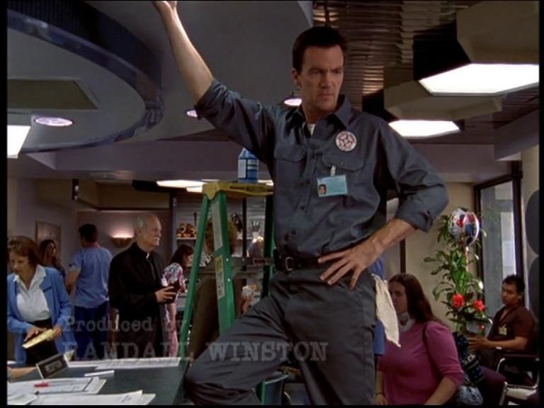
A
                    B
                        A
               B
                        C
                         D
                       C
                      A


                               49
                    50
                       51
             52
                       53
                        54
                      55
                     56


                   Thread
  A

                                                                Thread
  B

                                                                                                                                           Thread
  C

                       A
                     A
                        A
                        B
                         B
                                C
                      C


                               49
                    51
                       56
                       50
                        52
                                53
                     55

                                    Thread
  A
  Shots
                                            Thread
  B
  Shots
                                       Thread
  C
  Shots


Figure 2: Editing structure in a video: Shots are the atomic entities in editing patterns. Each image displays one
frame from a shot with its representative shot number written in yellow. Threads are interlaced repetition of shots
in a temporal neighbourhood. Shots in threads appear to repeat themselves. For example, shots 49, 51, 56 form one
thread A, while shots 50, 52 form thread B and 53, 55 form thread C. It is also common for some shots to be not part
of any threads (shot 54). Multiple single shots and threads form a scene and an episode is a collection of all scenes.
A scene typically consists of multiple intertwined shot thread                                                    An example of this type of must-not-link is shown in the top
patterns.                                                                                                         row of Figure 1.
   To partition an episode into scenes, we employ the                                                             2. ABAB threading patterns: A simple alternating
method of [28]. This locates scene boundaries by optimizing                                                       threading pattern such as “ABAB ” typically contains differ-
a cost function such that the within-scene content similarity                                                     ent characters in the threads A and B. In such patterns, we
is maximized while the between-scene similarity is small.                                                         form must-not-link constraint between every track in thread
The cost is based on shot appearance cues in the form                                                             A versus every track in thread B. Shots 49-52 in Figure 2
of colour histograms, and video editing structure in the                                                          show an example of this pattern.
form of shot threads where scene boundaries are placed to
                                                                                                                  3. Complex threading patterns: The simple rule ap-
minimize breaking of threads. The method uses dynamic
                                                                                                                  plied to “ABAB ” does not generalize to more complex pat-
programming to efficiently determine the optimal scene
                                                                                                                  terns like “ABCACABCA”. Nevertheless, they can be used
boundary localization, and also to automatically determine
                                                                                                                  to form must-not-link pairs as follows. First, we construct
the number of scenes. Note that scene boundaries are
                                                                                                                  all possible pairs where the face tracks originate from differ-
restricted to only occur at shot boundaries.
                                                                                                                  ent threads. Then we compute the face descriptor distance
   Scene partitioning allows us to simplify the large problem
                                                                                                                  within each pair and discard pairs where the distance is be-
of clustering about 500 tracks to dealing with only 20-40
                                                                                                                  low a given threshold. The remaining pairs are considered
tracks at a time. We show that by first clustering within
                                                                                                                  as must-not-link samples. Shots 53-56 in Figure 2 show ex-
scenes, we can build pure clusters more effectively than clus-
                                                                                                                  amples of this case.
tering directly across an episode and, in turn, these within
                                                                                                                     Negative pairs play an important role in our two stage
scene clusters are more suitable for between scene clustering
                                                                                                                  clustering approach. For the first part of clustering within a
than the original tracks.
                                                                                                                  scene, negative pair face descriptor distances are reset to ∞.
                                                                                                                  In the second stage of clustering across scenes, negative pairs
4.    THE CLUSTERING PROCESS                                                                                      are used to train discriminative models between clusters.
  We follow a three-step procedure to obtain the final face                                                       4.2             Part 1 Clustering: within a scene
track clusters: (1) obtain must-not-link face track pairs (neg-
ative pairs) using the shots and threading structure of the                                                          For a given episode, consider a scene s. Let T = {ti } be
video, (2) group the face tracks within each scene (part 1                                                        the set of face tracks in scene s. We represent a face track ti
clustering), and (3) merge the obtained scene level clusters                                                      by its appearance descriptor φi ∈ RD×1 . Given the video-
at the episode level (part 2 clustering). In this section, we                                                     editing structure and the cannot-link constraints described
explain the details related to each stage of the proposed                                                         above, we first set distances of track pairs which belong to
method. For readability, details of the face tracking and                                                         the cannot-link category to ∞.
feature extraction are postponed until Section 7.                                                                    Next, we exploit the fact that track pairs originating from
                                                                                                                  the same shot thread should allow for a relaxed distance
                                                                                                                  threshold, as the number of options to which they can be
4.1    Obtaining negative pairs                                                                                   matched is restricted. To obtain this threshold, we train a
   The process of obtaining negative pairs is a pre-processing                                                    linear classifier (SVM) which combines the descriptor dis-
step crucial for the success of the following clustering steps.                                                   tance d(·, ·) with the intersection-over-union measure γ(·, ·)
In this work, we consider three different sources for obtaining                                                   computed on average face locations, and predict a track pair
the must-not-link face tracks pairs.                                                                              as arising from the same person when
1. Temporal co-occurrence: As in previous works [3, 32],                                                                                      − wd · d(ti , tj ) + wγ · γ(ti , tj ) > θth .                           (1)
all pairs of temporally co-occurring face tracks are assumed
to depict different characters. This assumption holds in most                                                     Additionally, we learn a tight scene-level distance threshold
cases, but may fail e.g. if there are reflections from a mirror.                                                  θg to merge track pairs which are very similar in appearance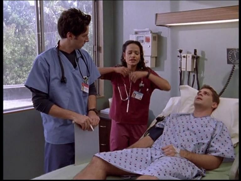
Correct
Merges
Could
Not
Merge
T457
T457
T480
T480
T09
T25
T104
T111
JD
JD
Ben
Ben
JD
JD
Janitor
Janitor
T48
T52
T208
T222
Full
Feature
Distance:
0.77
Frontal
Only
Distance:
0.85
Profile
Only
Distance:
0.87
Dr.
Kelso
JD
JD
Figure 4: Comparison of frontal and profile feature dis-
Dr.
Kelso
T169
T181
tances vs. full feature distance. As can be seen, com-
T117
T119
puting pose dependent features avoids making a wrong
merge.
Carla
Carla
Elliot
Elliot
Incorrect
Merge
obtain one Fisher vector over all face tracks in a single clus-
T123
T129
T119
T204
ter. Apart from improving the invariance of the features,
this reduces the number of comparisons that are otherwise
needed in typical agglomerative clustering.
Turk
Turk
Will
Dr.
Cox
Secondly, we partition the detections into two components
based on the head pose. This idea is very similar to the mix-
Figure 3: Output of Part-1 of our clustering method. ture model based approach of Deformable Parts Model [12]
Each image represents a track with given track id and and to more recent work [1, 23] that also considers pose ex-
label. Track ids indicate temporal closeness of each track plicitly in the face representation. In our paper, all frontal
in a pair. Left: examples of correct merges. Note tracks detections form one component and those having yaw angle
which contain quite different head poses (frontal and (rotation about a vertical axis) larger than 45o form another
near profile) are able to be merged. Right: examples component. We compute one high dimensional Fisher vector
of track pairs that could be merged but are not because for each of these components. Separating detections in this
of the head pose variation and lower temporal proximity way makes the task of comparing two clusters much easier
ruling out the thread based merging. The last pair shows as pose dependent features are compared separately for a
the first mistake that is made in episode 2 of Scrubs. pair of clusters.
Figure 4 shows our motivation behind this. We see that
but are not part of any thread. Track pairs ti , tj are classified
the complete feature has a smaller distance between two dif-
as belonging to the same class when
ferent characters, while splitting the feature into components
d(ti , tj ) = kφi − φj k < θg . (2) prevents this erroneous merge. Splitting a track or a cluster
according to pose not only prohibits false merges, but also
In Section 6, we show that this approach leads to a re- allows merging thresholds to be slightly looser in order to
duction in the number of clusters whilst keeping the cluster merge some other clusters which might not have merged.
purity very high. After this process, we update the must-not Note that it is not necessary that each cluster will have
link constraints using newly formed clusters. This helps us both frontal and profile parts. We observe that perform-
in the next stage of clustering. ing this split on clusters after within-scene clustering yields
Discussion. Clustering within a scene has been mentioned about 15-20% of clusters which contain only frontal faces
as a relatively easy problem [21], where a very simple ap- and thus an only frontal feature; about 5% of clusters consist
proach based on pair-wise track distances and hierarchical only of profile faces generating only profile features; while
agglomerative clustering (HAC) is used. Whilst this simple the remainder 75-80% form the bulk and have both frontal
technique works well for near frontal faces used in their case, as well as profile features. We design our merging strategy
the availability of better face detectors capable of detecting to take care of this. We merge two clusters if either of the
faces in various poses (as is our case), can lead to errors when distances is within threshold. So even if a cluster is missing
such a simple distance threshold based clustering method is one component, the other component is sufficient to merge
used. For example we observe that (Fig. 3), the distance the two clusters.
between two relatively frontal tracks of two different people Finally, rather than the distance metric based comparison
(right column row 4) could well be smaller than the distance from the previous part, we use exemplar Support Vector
between a frontal and a profile track of the same person (left Machine (e-SVM) classifiers as our scoring scheme. This
column rows 1 and 4). To facilitate merging of such tracks lets us use the negative information obtained from the video
of the same person with varying poses, we first employ the structure and part-1 clustering. In addition to this, we use
video editing structure to provide clues about clustering. the tracks from YouTube Faces In The Wild dataset [30] as
The use of spatial overlap from the thread structure allows stock negatives. We train one e-SVM per cluster and test it
us to lower the threshold for merging tracks of the same on all other clusters. The e-SVM is trained separately for
person within a thread (left column rows 1 and 4) before frontal and profile components.
merging tracks of different people (right column row 4). Calibration. The e-SVM scores are uncalibrated, thus
finding one threshold for merging clusters is impossible. To
4.3 Part 2 Clustering: across scenes overcome this problem, we normalize these scores using a
Given the scene-level clusters, we now move towards merg- sigmoid function.
ing them at the episode level. Towards this goal, we take
three important steps. First, to achieve a compact and pow- 1
erful descriptor, we extend the video pooling idea of [19] to φ(x) = . (3)
1 + exp(−ax + b)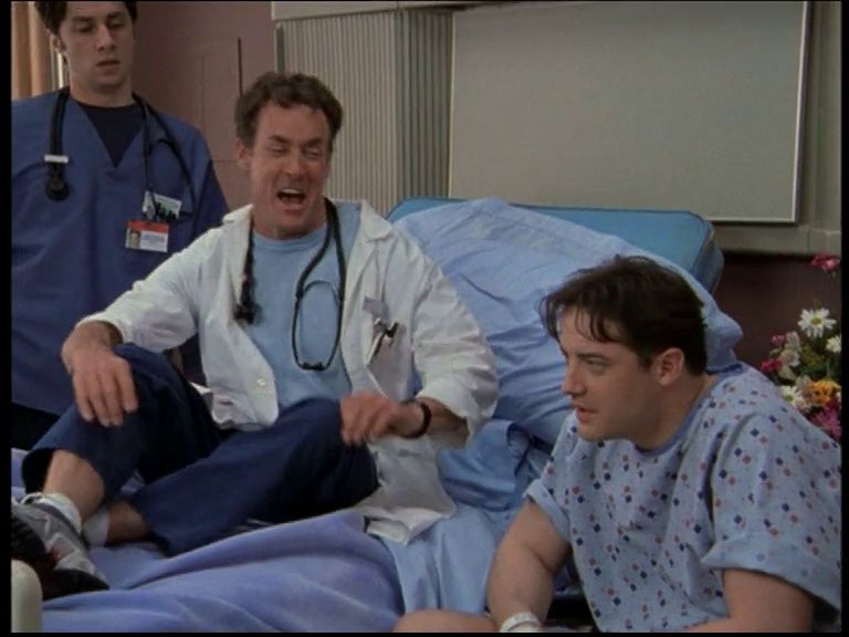
We wish to learn parameters a and b on a training episode.     Table 1: Statistics for the Scrubs face track data set
However, as the number of training samples to learn these        along with video-editing structure cues.
parameters is small, we use scores from all e-SVMs in the                               SCR-1 SCR-2 SCR-3 SCR-4 SCR-5 SCR-23
training episode and adapt them for a particular e-SVM us-        shots                  450     370    379    319    360    315
ing the score statistics                                          threads                91       70    79      53     73     69
                                                                  scenes                 27       21    24      25     23     21
        ak = α · µ(Sk )/σ(Sk ) and bk = β · 1/σ(Sk )      (4)
                                                                  named char.            17       12    15      17     16     19
where Sk is the set of e-SVM scores of all other clusters ob-     tracks for named       495     413    376    365    404    419
tained for an e-SVM model k and µ(·) and σ(·) compute the         shots in thread        295     242    260    223    264    242
mean and standard deviation respectively. We optimize for         tracks in thread       340     271    254    230    279    309
parameters α{f,p} and β {f,p} (respectively for frontal and       negs in-shot           232     192    116    212     222   310
profile models) such that we maximize the number of cor-          negs abab thread       136     104    114     88     174   316
                                                                  negs complex thread   1146     432    370    552    1078   596
rectly identified positive pairs and at the same time keep the
erroneous merges at zero.
   Please note that while we use e-SVMs and supervised           Table 2: Statistics for the Buffy face track data set along
training, there is no manual effort in gathering the labels as   with video-editing structure cues.
the negative data is mined automatically. Thus the method                             BF-1 BF-2 BF-3           BF-4   BF-5   BF-6
is fully automatic and unsupervised.                              shots                   678     616    820    714    675   745
                                                                  threads                 121     114    165    120    105   151
                                                                  scenes                  37       35    37     48      39    37
5.    EVALUATION PROTOCOL
                                                                  named char.             11       15    13     15      18    18
                                                                  tracks for named        630     779    973    668    646   842
5.1   Dataset information
                                                                  shots in thread         419     383    550    413    363   494
  We evaluate our techniques on two varied TV series              tracks in thread        449     552    668    425    408   592
datasets consisting of a sitcom Scrubs and a fantasy
                                                                  negs in-shot             282    620   752     216    192   582
drama Buffy the Vampire Slayer.                                   negs abab thread         176    240   172     58     170   164
Scrubs: In this sitcom, the story of the protagonist takes        negs complex thread     1742   1672   1916    212    712   4114
place primarily at a hospital (and his apartment) providing
many challenging scenarios such as: large number of back-        to perform clustering with no errors. For a given clustering C
ground characters, characters moving through corridors, etc.                                1 X
For the evaluation, we pick season 1, episodes 1–5 (SCR-1,                       W CP =           nc · purityc              (5)
                                                                                           N c∈C
. . ., SCR-5). We chose episode 23 (SCR-23) towards the end
of the season to train our parameters. For completeness, we      where each cluster c contains nc elements and its purity is
also show clustering results for this episode.                   measured as a fraction of the largest number of tracks which
Buffy the Vampire Slayer: The series, categorized as             belong to the same character to the number of tracks in the
a supernatural drama, presents multiple challenges from il-      cluster nc . N denotes total number of tracks in the video.
lumination, magic (character duplication), fast action, etc.     Operator Clicks Index (OCI-k) [13] Along with WCP,
While another dataset on Buffy tracks [3] has been used          we also report the clustering quality in terms of the num-
for face clustering before, we cannot use it since the data      ber of clicks required to label all the face tracks for a given
is obtained from multiple episodes and essentially treats        clustering. The lower and upper bounds for this metric are
face tracks as independent data points. The face tracks in       determined by the number of characters and face tracks, re-
our scheme have strong ties to the video-editing structure       spectively.
and benefit most when the entire episode is analyzed. We            An advantage of this measure is that it simultaneously
pick season 5, episodes 1–6 (BF-1, . . ., BF-6) and select one   incorporates the number of clusters and cluster quality in
episode (BF-4) for learning the parameters and thresholds.       one number. However, the advantage is also a drawback,
   Face tracks are obtained automatically and then labelled      since we can argue that correcting an error in clustering is
manually to obtain ground truth. We label all primary char-      not equivalent to labelling a pure cluster. A single click
acters and assign all background characters a single label.      corresponds to the effort needed to correctly label an in-
These background characters are not considered for evalua-       dividual face track in a wrong cluster, or all tracks in one
tion in our case. More details on how we obtain tracks and       cluster. For example, if we have 19 pure clusters (i.e. con-
compute features are discussed in Section 7.                     taining only tracks of the same character) and one cluster
                                                                 of 15 more data samples of which 5 are wrongly clustered
Table 1 and 2 present statistics on the Scrubs and Buffy
                                                                 samples, OCI-k needs a total of 25 (20 clusters + 5 errors)
data sets respectively. We show the number of video-editing
                                                                 clicks to label all face tracks correctly.
elements (shots, threads and scenes), and the number of
tracks in the episode. We also display the number of shots
and tracks which are part of a shot thread. The final section    6.    EXPERIMENTS
of the tables presents the number of mined negative pairs.         We now evaluate the performance of our method and com-
                                                                 pare it against different baseline approaches.
5.2   Evaluation criteria
  We use two measures to evaluate the quality of clustering:     6.1    Negative Pairs
Weighted Clustering Purity (WCP) The weighted                      In the first stage of our clustering, we form negative links
clustering purity (WCP) is our primary measure as we want        between different tracks. Here we compare our strategy de-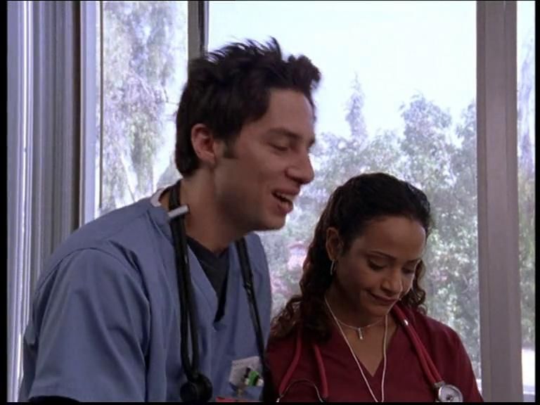
SCR−2: Scene: 8 nFT = 22                        SCR−3: Scene: 7 nFT = 14
scribed in Section 4.1 to previous methods of finding nega-                1                                            1
tives only by temporal co-occurrence. Tables 1 and 2 show
that our method obtains significantly more negatives than                 0.8                                          0.8

                                                                    WCP

                                                                                                                 WCP
just the pairs of temporally co-occurring tracks as negatives.
                                                                                                                                                    HAC curve
   For example, on the first episode of Scrubs (SCR-1), our               0.6                                          0.6                          Baseline
                                                                                                                                                    Proposed
method finds 1146 negative pairs in complex threads and 136
                                                                                 5      10        15        20               2    4     6     8    10   12   14
pairs in simple threads in addition to only 232 pairs found                             #clusters                                        #clusters
by temporal co-occurrence in a shot.
                                                                    Figure 5: Within-scene clustering results showing the
6.2    Clustering within a scene                                    number of clusters vs. WCP for episode 2 scene 8; and
                                                                    episode 3 scene 7. nFT is the number of face tracks in the
   Our goal for the clustering is to minimize the number of
                                                                    scene. Similar results for the other scenes are available
clusters while maintaining a very high cluster purity. Our
                                                                    in the supplementary material.
parameter selection using the training episode is tuned to-
wards this goal.                                                    dependent features reduce the number of clusters without
   As discussed in Section 4.2, within-scene clustering is per-     compromising on the cluster purity.
formed using both a tight global distance threshold, and also          A baseline for this part is to run hierarchical agglomerative
a relaxed threshold learned for tracks within threads which         clustering (HAC) on the entire episode. As in the previous
incorporates both appearance and spatial overlap measure-           section, this resembles the approach followed in [21]. Ad-
ments.                                                              ditionally [3] also followed a similar approach for clustering
   We compare to a strong baseline algorithm that merges            faces. As can be seen, the OCI-k click index is much lower
tracks using agglomerative clustering assisted by negative          than the baseline. E.g. on episode 4 we reduce 365 original
information. The threshold for the baseline is also learnt          clusters to 147 while the number of clusters obtained by the
on the training episode. This baseline is similar to that of        baseline method (182) is in fact more than that obtained by
previous works, e.g. [21].                                          the first stage of our proposed method. Both these trends
   As can be seen from Table 3 row 3 and 4 for the Scrubs           can also be observed on episode 2 where we reduce from 413
dataset, our strategy significantly reduces the number of           to 185 while the baseline is in fact worst than our part 1 208
clusters. For example, in the second episode of the Scrubs          and 202 respectively.
dataset (SCR-2), we manage to halve the number of clusters             We see a similar effect on the Buffy dataset as well where
from 413 (i.e. the original number of tracks) to 202. Similar       a significant reduction in the number of clusters is obtained
dramatic reductions can also be found in SCR-4 (365 to 181)         without any loss of purity (Tab. 4 rows 5 and 6).
and SCR-5 (404 to 217).                                                We show the results of clustering on the full episode in
   On the Buffy dataset, Table 4, we are able to reduce the         Figure 6. Similar to Figure 5, we plot the HAC curve and
number of clusters by more than 100 while maintaining clus-         mark the point at which the baseline stops. Our proposed
ter purity. This suggests that our proposed usage of video-         two-stage method achieves higher reduction in the number
editing structure is widely applicable to other TV series.          of clusters whilst maintaining the purity of the clusters. We
   We outperform the baseline on both datasets (rows 3 vs.          include the figure for the Buffy data set in the supplementary
4), reducing the number of clusters but without sacrificing         material.
cluster quality or increasing the number of clicks required to
label these clusters.
   Tracks can be fragmented due to face detection drop-out          7.          IMPLEMENTATION DETAILS
or temporary occlusion. This often presents quite an easy             We now discuss a few implementation details such as
clustering situation as the face descriptors can be quite sim-      face detection, tracking and representation which are a
ilar for the track portions. Also, clustering within a thread       pre-cursor for our task of face track clustering.
can be relatively easy. The baseline often copes with these
cases, and the proposed method goes beyond the baseline.            Face detection. This is the most important step of the
   Figure 5 shows examples of the within-scene clustering           pipeline. Compared to frontal detections, detecting faces in
on two scenes. We plot the hierarchical agglomerative clus-         extreme poses (profile, even the back of the head) remains
tering (HAC) purity obtained at every cluster number and            very challenging. However, the inability to detect these faces
overlay our baseline performance at the best possible thresh-       can cause fragmentation of tracks, making the clustering
old. We also show that our proposed method outperforms              task difficult. Furthermore, false positive face detections –
the baseline.                                                       frequently occurring with non-frontal detectors – are another
   Note, within-scene comparison figures for all scenes of one      problem affecting the tracking output.
episode are included in the supplementary material.                    To overcome these limitations we propose two solutions.
                                                                    First, we run the upper-body detector [8] on every frame and
6.3    Clustering across scenes                                     restrict the face detections to the upper-body region address-
                                                                    ing false positives. Second, to achieve high recall, in addi-
  In this section we look at effects of the clustering strategies
                                                                    tion to the OpenCV Viola-Jones face detectors (frontal and
discussed in Section 4.3.
                                                                    profile), we use the head detector of [17] designed to detect
  As can be seen from Table 3 for the Scrubs dataset, our
                                                                    a human head in frontal as well as extreme poses (frontal-
method significantly reduces the number of clusters while
                                                                    left/right, profile-left/right and even the back of head). This
keeping the cluster purity very close to 1 (rows 5 and 7).
                                                                    detector is based on the Deformable Parts Model of [11].
We evaluate our scheme of comparing pose dependent fea-
tures for clusters to that of using a single feature for the        Face tracking. Face tracks are formed by performing the
entire cluster (Tab. 3 rows 6 and 7). Our proposed pose-            data association technique described in [10]. Specifically, we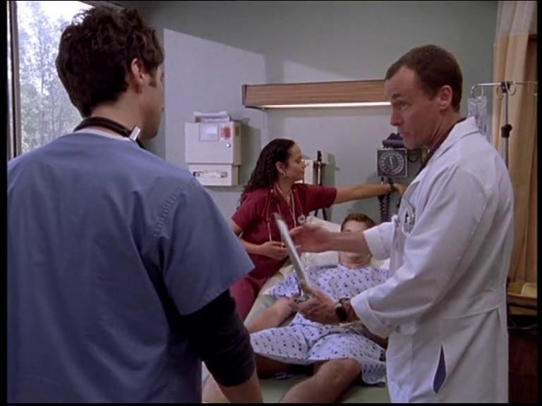
Table 3: Clustering results on Scrubs. Episode SCR-23 is used for learning parameters.
Episodes SCR-1 SCR-2 SCR-3 SCR-4 SCR-5 SCR-23
1 #tracks 495 413 376 365 404 419
2 #ideal 17 12 15 17 16 19
Measures NC WCP OCI-k NC WCP OCI-k NC WCP OCI-k NC WCP OCI-k NC WCP OCI-k NC WCP OCI-k
Within scene clustering
3 Baseline 319 0.996 321 233 1.000 233 222 0.997 223 200 1.000 200 251 1.000 251 232 1.000 232
4 Proposed part-1 293 1.000 293 202 0.994 205 205 0.998 206 181 1.000 181 217 1.000 217 212 1.000 212
Full episode clustering
5 Baseline 287 1.000 287 208 0.998 209 196 0.995 198 182 1.000 182 246 1.000 246 208 1.000 208
6 SVM full feature 293 1.000 293 202 0.994 205 205 0.998 206 181 1.000 181 217 1.000 217 210 1.000 210
7 Proposed part-2 244 0.992 248 185 0.992 188 179 0.992 182 147 0.998 148 198 0.998 199 173 1.000 173
SCR−1 SCR−2 SCR−3
1 1 1
0.9 0.9 0.9
0.8 0.8 0.8
WCP
WCP
WCP
0.7 HAC curve 0.7 HAC curve 0.7 HAC curve
Ideal Ideal Ideal
0.6 Baseline 0.6 Baseline 0.6 Baseline
Proposed Proposed Proposed
0.5 0.5 0.5
100 200 300 400 100 200 300 400 100 200 300
#clusters #clusters #clusters
SCR−4 SCR−5 SCR−23
1 1 1
0.9 0.9
0.8 0.8 0.8
WCP
WCP
WCP
HAC curve
0.7 HAC curve 0.7 HAC curve
Ideal
Ideal Ideal
Baseline 0.6 Baseline Baseline
0.6 0.6
Proposed Proposed Proposed
0.5 0.5
100 200 300 100 200 300 400 100 200 300 400
#clusters #clusters #clusters
Figure 6: The number of clusters versus the cluster purity for each episode in the Scrubs dataset. It can be observed
that our approach consistently results in a smaller number of clusters with similar purity than the baseline. The
HAC curve illustrates the clustering results obtained with standard agglomerative clustering with different thresholds.
Note that one cannot directly select an operating point from this curve, since the corresponding threshold is not
known (threshold needs to be learned using holdout data). Similar curves for the Buffy dataset are available in the
supplementary material.
use the Kanade-Lucas-Tomasi (KLT) [24] tracker to obtain tor (67584) which is reduced to a very low dimension (128)
feature tracks intersecting with face detections. To achieve using discriminative dimensionality reduction. To make the
robust performance, feature tracking is carried out in both descriptor more robust, dense SIFT features are computed
forward and backward directions. After linking detections on horizontal flips of every detection and pooled into the
in a track, misses between two detections are obtained by same Fisher vector. We use the projection matrix learned
interpolation based on two neighbouring detections and the on “YouTube Faces Dataset” as described in [19] to perform
spread of KLT feature tracks in that frame. To remove false the dimensionality reduction.
positive face tracks, we follow an approach similar to [15].
We form a track level feature vector using different track
statistics: track features track length, ratio of track length 8. CONCLUSIONS AND EXTENSIONS
to number of detected faces in a track, mean and standard In this paper we have presented a method for unsuper-
deviation of head detection scores. This feature vector is vised face track clustering. Unlike many previous methods,
then used to classify the track using a linear-SVM classi- we explicitly utilise video structure in clustering. In partic-
fier trained on ground truth false positive and true positive ular, we take advantage of shot threads, which allow us to
tracks obtained from data distinct from that used in this form several must-not-link constraints and to use optimized
work. similarity thresholds within the threading patterns. In the
experiments, we showed that our approach can greatly re-
Face representation. Fisher vector based representation duce the number of face tracks without making almost any
of face tracks was recently introduced in [19]. The descrip- mistakes in the process. Such an output is a much bet-
tor is computed by first extracting dense SIFT [16] features ter starting point for many supervised methods as well as
for every detection in a track and then pooling them to- manual track labelling. In addition, we illustrate a clear im-
gether to form a single Fisher vector feature for the whole provement over the baseline that also utilises video structure
track. The resulting descriptor is a high dimensional vec- in the form of shots and scenes.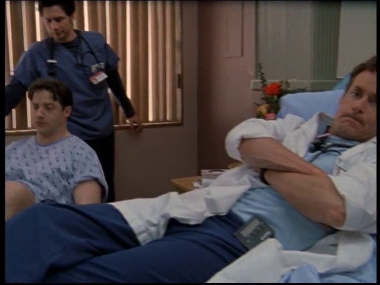
Table 4: Clustering results on Buffy. Episode BF-4 is used for learning parameters.
       Episodes            BF-1                BF-2                  BF-3                BF-4               BF-5                BF-6
 1      #tracks              630                779                  974                  668                646                 843
 2      #ideal               11                 15                   13                   15                 18                  18
       Measures      NC WCP OCI-k NC WCP OCI-k NC WCP OCI-k NC WCP OCI-k NC WCP OCI-k NC WCP OCI-k
                                                  Within scene clustering
 3    Baseline     537 1.000       537   697 1.000    697    852 1.000       852   567 1.000    567   584 0.999    585    761 1.000    761
 4 Proposed part-1 501 1.000       501   655 1.000    655    814 1.000       814   524 1.000    524   550 0.999    551    717 1.000    717
                                                   Full episode clustering
 5    Baseline     534 1.000       534   688 1.000    688    852 1.000       852   566 1.000    566   575 0.999    576    751 1.000    751
 6 Proposed part-2 466 1.000       466   598 1.000    598    730 1.000       730   494 1.000    494   507 0.998    508    643 1.000    643

  We have concentrated in this paper on clustering using                   [15] A. Kläser, M. Marszalek, C. Schmid, and A. Zisserman.
faces alone. However, since a scene forms a short and coher-                    Human focused action localization in video. In
ent story segment, it is justified to assume that the appear-                   International Workshop on Sign, Gesture, Activity, 2010.
ance (e.g. of hair, clothing, etc.) of the characters do not               [16] D. Lowe. Distinctive image features from scale-invariant
                                                                                keypoints. IJCV, 60(2):91–110, 2004.
change much within one scene. This can be used to assist
                                                                           [17] M. Marin-Jimenez, A. Zisserman, and V. Ferrari. “Here’s
the clustering, e.g. by relaxing distance thresholds or using                   looking at you, kid.” Detecting people looking at each other
appropriate weighting for different cues [21].                                  in videos. In Proc. BMVC., 2011.
                                                                           [18] J. Monaco. How to Read a Film: The World of Movies,
Acknowledgments                                                                 Media, Multimedia – Language, History, Theory. OUP
This work was supported by ERC grant VisRec no. 228180,                         USA, Apr 2000.
EU Project AXES ICT–269980, and a Royal Society Wolfson                    [19] O. M. Parkhi, K. Simonyan, A. Vedaldi, and A. Zisserman.
Research Merit Award.                                                           A compact and discriminative face track descriptor. In
                                                                                Proc. CVPR, 2014.
                                                                           [20] L. C. Pickup and A. Zisserman. Automatic retrieval of
9.   REFERENCES                                                                 visual continuity errors in movies. In Proc. CIVR, 2009.
 [1] B. Bhattarai, G. Sharma, F. Jurie, and P. Perez. Some                 [21] D. Ramanan, S. Baker, and S. Kakade. Leveraging archival
     faces are more equal than others: Hierarchical organization                video for building face datasets. In Proc. ICCV, 2007.
     for accurate and efficient large-scale identity-based face            [22] J. See and C. Eswaran. Exemplar Extraction Using
     retrieval. In ECCV Workshop, 2014.                                         Spatio-Temporal Hierarchical Agglomerative Clustering for
 [2] P. Bojanowski, F. Bach, I. Laptev, J. Ponce, C. Schmid,                    Face Recognition in Video. In ICCV, 2011.
     and J. Sivic. Finding actors and actions in movies. In Proc.          [23] G. Sharma, F. Jurie, and P. Perez. EPML: Expanded Parts
     ICCV, 2013.                                                                based Metric Learning for Occlusion Robust Face
 [3] R. G. Cinbis, J. J. Verbeek, and C. Schmid. Unsupervised                   Verification. In ACCV, 2014.
     metric learning for face identification in TV video. In Proc.         [24] J. Shi and C. Tomasi. Good features to track. In Proc.
     ICCV, 2011.                                                                CVPR, pages 593–600, 1994.
 [4] T. Cour, C. Jordan, E. Miltsakaki, and B. Taskar.                     [25] J. Sivic, M. Everingham, and A. Zisserman. “Who are
     Movie/script: Alignment and parsing of video and text                      you?” – learning person specific classifiers from video. In
     transcription. In Proc. ECCV, 2008.                                        Proc. CVPR, 2009.
 [5] T. Cour, B. Sapp, A. Nagle, and B. Taskar. Talking                    [26] T. J. Smith. An Attentional Theory of Continuity Editing.
     pictures: Temporal grouping and dialog-supervised person                   PhD thesis, University of Edinburgh, 2006. Unpublished
     recognition. In Proc. CVPR, 2010.                                          Doctoral Thesis.
 [6] T. Cour, B. Sapp, and B. Taskar. Learning from                        [27] M. Tapaswi, M. Bäuml, and R. Stiefelhagen. “Knock!
     ambiguously labeled images. In Proc. CVPR, 2009.                           Knock! Who is it?” Probabilistic Person Identification in
 [7] T. Cour, B. Sapp, and B. Taskar. Learning from partial                     TV Series. In Proc. CVPR, 2012.
     labels. J. Machine Learning Research, 2011.                           [28] M. Tapaswi, M. Bäuml, and R. Stiefelhagen. StoryGraphs:
 [8] M. Eichner and V. Ferrari. Better appearance models for                    Visualizing Character Interactions as a Timeline. In CVPR,
     pictorial structures. In Proc. BMVC., 2009.                                2014.
 [9] M. Everingham, J. Sivic, and A. Zisserman. “Hello! My                 [29] P. Wohlhart, M. Köstinger, P. M. Roth, and H. Bischof.
     name is... Buffy” – automatic naming of characters in TV                   Multiple instance boosting for face recognition in videos. In
     video. In Proc. BMVC., 2006.                                               DAGM-Symposium, 2011.
[10] M. Everingham, J. Sivic, and A. Zisserman. Taking the bite            [30] L. Wolf, T. Hassner, and I. Maoz. Face recognition in
     out of automatic naming of characters in TV video. Image                   unconstrained videos with matched background similarity.
     and Vision Computing, 27(5), 2009.                                         In Proc. CVPR, 2011.
[11] P. Felzenszwalb, D. Mcallester, and D. Ramanan. A                     [31] B. Wu, S. Lyu, B.-G. Hu, and Q. Ji. Simultaneous
     discriminatively trained, multiscale, deformable part model.               Clustering and Tracklet Linking for Multi-Face Tracking in
     In Proc. CVPR, 2008.                                                       Videos. In ICCV, 2013.
[12] P. F. Felzenszwalb, R. B. Grishick, D. McAllester, and                [32] B. Wu, Y. Zhang, B.-G. Hu, and Q. Ji. Constrained
     D. Ramanan. Object detection with discriminatively                         Clustering and Its Application to Face Clustering in
     trained part based models. IEEE PAMI, 2010.                                Videos. In CVPR, 2013.
[13] M. Guillaumin, J. Verbeek, and C. Schmid. Is that you?                [33] Y. Yusoff, W. Christmas, and J. Kittler. A Study on
     Metric learning approaches for face identification. In Proc.               Automatic Shot Change Detection. Multimedia
     ICCV, 2009.                                                                Applications, Services and Techniques, 1998.
[14] E. Khoury, P. Gay, and J.-M. Odobez. Fusing Matching
     and Biometric Similarity Measures for Face Diarization in
     Video. In ICMR, 2013.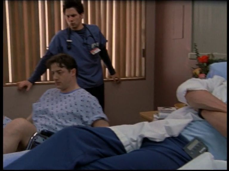

You can also read