Analysing and Maximising the Effectiveness of Test, Trace, and Isolate Strategies
←
→
Page content transcription
If your browser does not render page correctly, please read the page content below
Analysing and Maximising the
Effectiveness of Test, Trace, and Isolate
               Strategies
Machine Learning and the Physical World - Group Project

              Maleakhi Wijaya (maw219)
                   Chuan Tan (ct538)
                 Jakub Mach (jm2175)

        Department of Computer Science and Technology
                   University of Cambridge

                        January 2021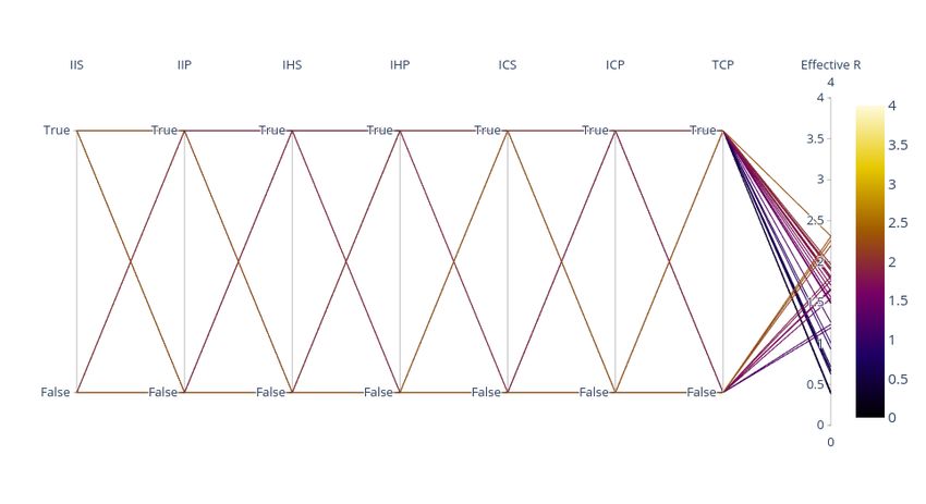
Abstract
The Test, Trace, and Isolate (TTI) explorer (tti-explorer) is a model used to sim-
ulate the spread of COVID-19 infection in the UK, given various TTI strategies and
non-pharmaceutical interventions (NPIs). This report seeks to analyse the mag-
nitude of effect of various TTI strategies and NPIs on the effective reproduction
number (effective R) of the disease and to derive optimal policies for containing
the outbreak. These objectives were achieved by employing sensitivity analysis
and optimisation methods on the tti-explorer simulator. Specifically, we used
global sensitivity analysis methods, amounting to grid and axis variations, to anal-
yse the impact of each factor in isolation; and the analysis of variance (ANOVA)
decomposition using the Gaussian process emulator, to examine the overall impact
of all factors, considering the interactions between them. We show that the Gaus-
sian process emulator enables rapid computation of ANOVA decomposition, thus
allowing us to present a more complete sensitivity analysis result that complement
prior work in the COVID-19 domain. Subsequently, we used random search, un-
constrained Bayesian optimisation, and constrained Bayesian optimisation to derive
an optimal policy for slowing the spread of the virus. We demonstrate the superi-
ority of Bayesian optimisation-based approaches over the random search, as they
obtained more optimal and sensible policies much faster.

                                     Codes
The codes written in Python is available at: https://github.com/maleakhiw/
gaussian-processes-tti-explorer.

                                         2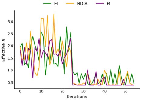
Contents
1   Introduction                                                                                                                                   4

2   Experimental Setup and Design Choices                                                                                                          4
    2.1 Simulator . . . . . . . . . . . . . . . . . . . . . . . . . . . . . . . . . . . . .                                                        4
    2.2 Sensitivity Analysis Factors . . . . . . . . . . . . . . . . . . . . . . . . . . . .                                                       5
    2.3 Policy Optimisation Factors . . . . . . . . . . . . . . . . . . . . . . . . . . . .                                                        6

3   Sensitivity Analysis                                                                                                                            7
    3.1 Grid and Axis Variation . . . . . . .          .   .   .   .   .   .   .   .   .   .   .   .   .   .   .   .   .   .   .   .   .   .   .    7
    3.2 Analysis of Variance Decomposition             .   .   .   .   .   .   .   .   .   .   .   .   .   .   .   .   .   .   .   .   .   .   .   13
         3.2.1 Background . . . . . . . . .            .   .   .   .   .   .   .   .   .   .   .   .   .   .   .   .   .   .   .   .   .   .   .   13
         3.2.2 Experiment Results . . . . .            .   .   .   .   .   .   .   .   .   .   .   .   .   .   .   .   .   .   .   .   .   .   .   13
    3.3 Causal Analysis . . . . . . . . . . .          .   .   .   .   .   .   .   .   .   .   .   .   .   .   .   .   .   .   .   .   .   .   .   16

4   Policy Optimisation                                                                                                                            17
    4.1 Unconstrained Optimisation .       .   .   .   .   .   .   .   .   .   .   .   .   .   .   .   .   .   .   .   .   .   .   .   .   .   .   18
         4.1.1 Random Search . . . .       .   .   .   .   .   .   .   .   .   .   .   .   .   .   .   .   .   .   .   .   .   .   .   .   .   .   18
         4.1.2 Bayesian Optimisation       .   .   .   .   .   .   .   .   .   .   .   .   .   .   .   .   .   .   .   .   .   .   .   .   .   .   19
    4.2 Ablation Studies . . . . . . . .   .   .   .   .   .   .   .   .   .   .   .   .   .   .   .   .   .   .   .   .   .   .   .   .   .   .   21
    4.3 Constrained Optimisation . . .     .   .   .   .   .   .   .   .   .   .   .   .   .   .   .   .   .   .   .   .   .   .   .   .   .   .   23

5   Conclusion                                                                                                                                     24

6   Appendices                                                                                                                                     25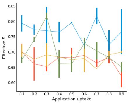
Machine Learning and the Physical World – Group Project

1     Introduction
The COVID-19 pandemic has presented a significant challenge to policymakers. The SARS-
CoV-2 virus is difficult to control due to its high reproduction rate, high asymptomatic rate, and
frequent unavoidable occurrences of super-spreading events [3, 8, 18]. During the initial stages
of the outbreak, policymakers could rely on standard, less strict strategies, such as test-trace-
isolate (TTI) strategies and COVID-19 health protocols [19, 27]. Nevertheless, the epidemic
continues to escalate, necessitating other strict non-pharmaceutical interventions (NPIs), such
as school closures and working from home. Studies have shown that despite the need for a strict
policy to slow the spread of the virus, such a policy may cause significant disruption to societies
(e.g., psychological distress and mental health problems [6, 13, 26]) and to the country’s econ-
omy [1]. Therefore, it is crucial for policymakers to develop policies that balance effectiveness
and strictness.
    This report has two primary objectives. Firstly, to evaluate the magnitude of effect of var-
ious TTI strategies and NPIs on the effective reproduction number (effective R) of the disease
– that is, the average number of secondary cases per infectious case in a population comprising
both susceptible and non-susceptible hosts [14]. Secondly, it aims to derive an optimal policy
that has the greatest effect on the reduction of effective R, while considering available resources
and restrictions (e.g., number of tests needed [7], the inability of essential workers to work from
home [4]). We implemented various global sensitivity analysis methods, amounting to grid and
axis variations that analyse factors in isolation, and analysis of variance (ANOVA) decomposi-
tion, which analyses factors while considering the interactions between them. Subsequently, we
implemented random search, unconstrained Bayesian optimisation, and constrained Bayesian
optimisation for the policy optimisation problem. Both sensitivity analysis and policy optimisa-
tion methods are applied on the simulator, tti-explorer [12,27], a model used to simulate the
spread of COVID-19 infection in the UK given various TTI strategies and NPIs as parameters.
    The remainder of the report is organised as follows. Section 2 describes the assumptions
and setup of the experiments. Section 3 discusses global sensitivity analysis and causal analysis
results. Section 4 presents optimal policies obtained by various optimisation methods. It then
compares the performance of different optimisation methods, identifying their strengths and
weaknesses. Finally, Section 5 summarises the main findings of the study.

2     Experimental Setup and Design Choices
This section describes tti-explorer and how it was adapted for the experiments. Subse-
quently, it lists and defines important factors considered in both the sensitivity analysis and
policy optimisation experiments.

2.1    Simulator
The simulator, tti-explorer was developed by Kucharski et al. [12] and He et al. [27] to
simulate the spread of COVID-19 in the UK, given various parameter configurations related
to different TTI strategies and NPIs as inputs. Each time a simulation is run, the simulator
performs three main steps, visualised in Figure 1.
    1. The first step involves generating initial cases. Each case describes an individual that can
       be under or over 18, COVID positive or negative, and with or without symptoms, based

                                                 4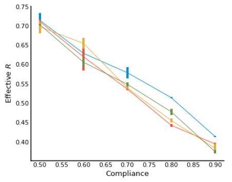
Machine Learning and the Physical World – Group Project

       on configured probability distributions. In the experiments, we generated 10,000 initial
       cases.
   2. The next step generates social contacts for each initial case. To select the number of con-
      tacts, the simulator samples the BBC Pandemic dataset [11], which contains the number
      of daily contacts in different situations collected from UK volunteers.
   3. Finally, given a particular strategy (e.g. test-based TTI with NPI of stringency level S3),
      each case is passed through the simulator, which computes various metrics, including
      the effective R, number of tests needed, number of app traces, number of manual traces,
      and number of person days quarantined1 . The results of each case are then collected and
      averaged to return the output of the simulator.
   The simulator is treated as a function that maps strategy inputs to the aforementioned output
metrics. These functions are then approximated using Gaussian process surrogate models for
several experiments described in Sections 3 and 4.

Figure 1: The three main steps of the simulation: generate cases, generate social contacts, and compute required
metrics given a particular strategy.

2.2     Sensitivity Analysis Factors
We identified 13 parameters that strongly influence the effective R and can be used to influence
decision-making and inform policies [9]. The parameters are grouped into general factors,
policy factors, and compliance factors (listed in Table 1).

General factors The general factors contain variables that provide an overarching view of the
simulation. These include the probability of being under 18 (p_under18) and secondary attack
rates (SARs) (home_sar, work_sar, other_sar). These provide insights into how the general
properties of a population affect the effective R.

Policy factors The policy factors are variables that can be influenced through policy-making.
They include the proportion of adults working from home (wfh_prob), maximum social con-
tacts (max_contacts), and quarantine length (quarantine_length). Policy factors provide
insights into the success of different policies at preventing the spread of the virus.
   1 Full   list of output metrics are described in [27].

                                                            5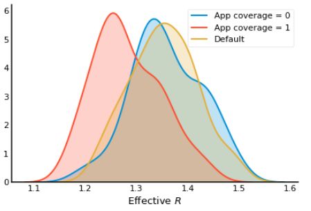
Machine Learning and the Physical World – Group Project

Compliance factors Finally, compliance factors are proxy variables that capture human be-
haviour, such as the level of compliance (compliance) and tracing application coverage (app_cov).
They provide an insight of policy limitations due to human behaviour.

                                                   Variables
                                                  p_under18
                                                   home_sar
                            General Factors
                                                   work_sar
                                                  other_sar
                                                   wfh_prob
                                              go_to_school_prob
                                                 max_contacts
                             Policy Factors   quarantine_length
                                                testing_delay
                                              manual_trace_delay
                                               app_trace_delay
                                                  compliance
                           Compliance Factors
                                                   app_cov
Table 1: Grouping of factors into three different groups: general, policy, and compliance factors. A detailed
description of each parameter is presented in Table 6.

2.3    Policy Optimisation Factors
For the optimisation task we selected all parameters influenceable through policymaking. In
total this was 14 policy parameters (set out in Table 2) that capture the functional essence of the
variable groups set out in Section 2.2. Notably, there are several parameters which cannot be
affected via policies. For example, SARs are more related to the infectiousness of a viral strain.
Consequently, these parameters are excluded.

                        Variables                                        Type
                   go_to_school_prob                              Float, range:[0,1]
                        wfh_prob                                  Float, range:[0,1]
             isolate_individual_on_symptoms                  Boolean, range: [True, False]
             isolate_individual_on_positive                  Boolean, range: [True, False]
             isolate_household_on_symptoms                   Boolean, range: [True, False]
             isolate_household_on_positive                   Boolean, range: [True, False]
              isolate_contacts_on_symptoms                   Boolean, range: [True, False]
              isolate_contacts_on_positive                   Boolean, range: [True, False]
               test_contacts_on_positive                     Boolean, range: [True, False]
                   do_symptom_testing                        Boolean, range: [True, False]
                   do_manual_tracing                         Boolean, range: [True, False]
                     do_app_tracing                          Boolean, range: [True, False]
                      max_contacts                              Integer, range: [1,20]

                                                     6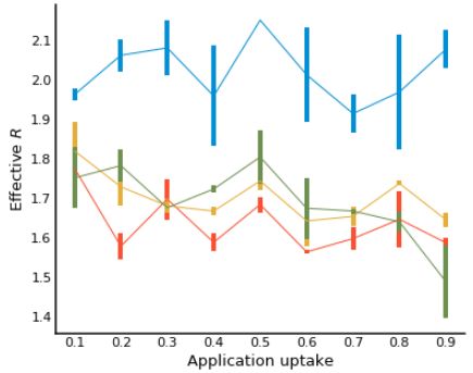
Machine Learning and the Physical World – Group Project

                         quarantine_length                            Integer, range: [0,14]
Table 2: List of variables used for optimisation in Section 4. A detailed description of each parameter is presented
in Table 7.

3     Sensitivity Analysis
This section details the global sensitivity analyses conducted to evaluate the magnitude of each
parameter effect on the effective R. We performed two sets of analysis: one analysing the effect
of each variable in isolation and another that included the interactions between them. In addition
to effective R, we measured the variables’ impacts on the number of tests needed, number of app
traces, number of manual traces, and number of person days quarantined. These analyses serve
as a basis for determining resources that could be limited in practice, thus helping to identify
factors to target during policy optimisation in Section 4. We also performed causal analysis by
intervening directly in the simulator to understand the causal relationships between variables.

3.1     Grid and Axis Variation
The grid and axis variation are two simple strategies that can be used to perform global sen-
sitivity analysis [17]. Grid variation refers to trying all possible combinations of parameters
in the group to determine their contributions. Conversely, axis variation refers to trying one
parameter at a time, while keeping all remaining parameters fixed. Both methods are used to
measure the impact of a parameter on a function in isolation, as they cannot detect interactions
between parameters [2]. Section 3.2 extends the experiments by considering more parameters,
while also considering the interactions between them.
     We selected several parameters to conduct sensitivity analysis, following the grouping and
reasoning discussed in Section 2. From Table 1, we selected nine parameters to vary in order
to analyse their impacts on the effective R: p_under18, home_sar, work_sar, other_sar,
wfh_prob, go_to_school_prob, max_contacts, compliance, and app_cov. The simula-
tions were conducted five times for each experiment and we reported the mean and 95% confi-
dence interval.

Age We varied p_under18 from 0.0 (all working adults) to 1.0 (all school-going children) to
investigate how age affects the effective R. The results are plotted in Figure 2. Generally, we
observed that age plays an important role in influencing the disease’ effective R. Specifically,
the higher the p_under18 (higher population of school-going children), the lower the effective
R. Further observation on the BBC Pandemic dataset suggests that this phenomenon is caused
by the vast difference in the number of social interactions of under 18 individuals compared to
working adults. Social interaction of individuals under 18 is primarily restricted to household
members and schoolmates, while working adults come into contact with more individuals, for
example when meeting clients, travelling for work, and socialising with friends. This relation-
ship holds for different strictness environments, suggesting that age is an important parameter.

Work from home We varied wfh_prob from 0.0 (all working adults work from the office) to
1.0 (all working adults work from home) to evaluate how a work from home policy impacts the

                                                         7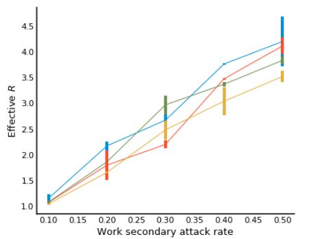
Machine Learning and the Physical World – Group Project

spread of COVID-19. Figure 2 shows a strong negative linear relationship between wfh_prob
and effective R at all five strictness levels of NPIs (S1-S5). Particularly, we observed a max-
imum reduction of 44% in the effective R, suggesting that a strict work-from-home policy is
effective at containing the pandemic.

Go to school Considering the previous result, it is unsurprising that go_to_school_prob
also affects the effective R. Indeed, Figure 2 depicts a positive linear relationship between
go_to_school_prob and the effective R. We observed a maximum increase of 17% in the
effective R. In Section 3.2, we observed that the hidden variable is the number of contacts with
which each individual comes into contact. Going to school increases the number of contacts,
which in turn results in a more drastic rise in the effective R.

Secondary attack rates We varied home_sar, work_sar, and other_sar from 0.0 (no sec-
ondary attack) to 0.5 (50% probability of secondary attacks given a positive case). Figure 3
shows a positive linear relationship between all SARs variables and the effective R for all five
levels of governmental measures (S1-S5). We observed that work_sar had the greatest effect,
followed by other_sar, and home_sar. The phenomenon makes sense as there are more social
contacts at work than at home or in other places.

Maximum contacts Since the previous analyses suggest that the number of social contacts
plays a large role in containing the virus, we varied the max_contacts from 2 to 20. We
observed a positive linear trend between it and the effective R, thus agreeing with the previous
analyses, as shown in Figure 4. Further analysis showing the importance of limiting contacts is
presented in Section 3.2.

Compliance Naturally, the more likely a person is to comply with rules and regulations, the
lower the effective R. Even in the least strict policy scenario (S1), we see that a 90% compliance
level helps reduce effective R by 25% in the absence of testing and tracing, as visualised in
Figure 4. This suggests that enacting fines and penalties to enforce compliance can significantly
help to reduce the effective R.

Application coverage We varied the app_coverage from 0.0 to 1.0, shown in Figure 4. We
observed that increasing application uptake slightly reduces the effective R, as tracing can be
carried out more quickly without delay. However, we noted that the difference between 0.0 and
1.0 app_coverage is minor, so this parameter is less significant than other parameters.

                                                8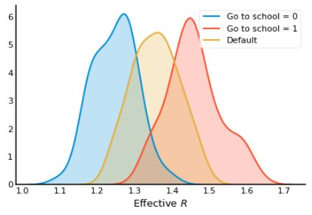
Machine Learning and the Physical World – Group Project

Figure 2: Left: Effect of varying the probability of under 18 on effective R. Middle: Effect of varying work from
home proportion on effective R. Right: Effect of varying go to school probability on effective R. Top to Bottom:
5 levels of governmental measures: S1-S5. The error bars are 95% confidence intervals.

                                                       9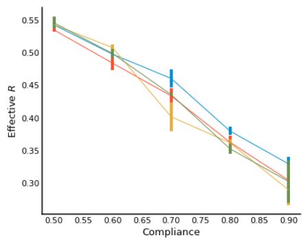
Machine Learning and the Physical World – Group Project

Figure 3: Left: Effect of varying the home secondary attack rate on effective R. Middle: Effect of varying the
work secondary attack rate on effective R. Right: Effect of varying the other secondary attack rate on effective R.
Top to Bottom: 5 levels of governmental measures: S1-S5. The error bars are 95% confidence intervals.

                                                       10
Machine Learning and the Physical World – Group Project
Figure 4: Left: Effect of varying the number of maximum contacts per day on effective R. Middle: Effect of
varying the compliance level on effective R. Right: Effect of varying the application coverage on effective R. Top
to Bottom: 5 levels of governmental measures: S1-S5. The error bars are 95% confidence intervals.
11Machine Learning and the Physical World – Group Project
We employed grid variation, varying the five levels of governmental measures (S1-S5) and
four TTI strategies: no TTI, trace on symptoms, trace on positive test and trace on positive
test with contacts testing. We observed their overall effects on the effective R, number of tests
needed, number of manual traces, number of app traces and number of total days quarantined.
The results are shown in Figure 5. The effective R plot demonstrates the benefits of TTI, through
a lower effective R compared to no TTI. Interestingly, the lowest effective R was achieved using
symptoms- and test-based TTI strategies, suggesting that trace on positive test with contacts
testing is not beneficial, despite its expense. From the other plots, we observed that the number
of traces and person days quarantined are significantly higher for the symptoms-based TTI
strategy than for other strategies. The overall high-level overview suggests that the test-based
TTI strategy is the most beneficial as it attains the minimum effective R with reasonable resource
requirements.
Figure 5: Impact on effective R and resource requirement of various TTI strategies across the five sets of gov-
ernmental measures, for 10,000 primary cases. The number of tests, manual traces, app traces, and person days
quarantined are in thousands.
12Machine Learning and the Physical World – Group Project
3.2 Analysis of Variance Decomposition
3.2.1 Background
Due to their simplicity, axis and grid variations cannot capture the interactions between vari-
ables. Consequently, we used the ANOVA decomposition method for a complete global sensi-
tivity analysis that can fully explore the input spaces, while considering the interactions between
parameters and nonlinear responses [24]. The ANOVA decomposition performs sensitivity
analysis by decomposing the variance of a target function into parts attributable to input param-
eters and their interactions. The magnitude of the effect of input to output is then calculated
relative to the variance in output caused by that input. More formally, the following equation
defines the ANOVA decomposition of the total variance into a combination of the variances of
the smaller functions, each representing the interactions between different inputs:
Var[g] = hg(x)2 i p(x) − hg(x)i2p(x)
= hg(x)2 i p(x) − g20
p p
= ∑ Var[gi(xi)] + ∑ Var[gi j (xi, x j )] + · · · + Var[g1,2,...,p(x1, x2, . . . , x p)]
i=1 i< j
The hg(x)i p(x) is the expectation of the function g(x) under the density p(x), which represents
the probability distribution of inputs we’re interested in. While gi (xi ) represent the impact of
a single variable, gi, j (xi , x j ) measures the effect of two variables interacting. It is common to
rescale the components with the total variance of the function; these rescaled components are
known as the Sobol indices:
var (g(x` )))
S` =
var (g(x))
Using the Sobol indices, we can evaluate the effect of each set of inputs on the output.
There are two metrics for quantifying these effects: main effects and total effects. The main
effects consider only summing the first-order Sobol indices to measure the magnitude of each
input. Conversely, the total effects also consider higher-order interaction terms of any order.
To compute both the main and total effects, we used Emukit [20]. We estimated the Sobol in-
dices using two methods: model-free Monte Carlo, which calculates these indices by sampling
the simulator directly [23], and model-based Monte Carlo, which calculates indices by sam-
pling a Gaussian process emulator [15]. For the experiments (see Section 3.2.2), we computed
10,000 evaluations for the model-free and model-based Monte Carlo approaches to estimate
the indices. Model-free Monte Carlo requires lengthy computation time, as each simulation run
takes around 1 second to complete, in total demanding over 10 hours of computation to estimate
the Sobol indices. Conversely, model-based Monte Carlo achieved comparable results within
a significantly shorter time of 15 minutes. This highlights the benefits of employing Gaussian
process emulator, which makes it feasible to employ variable-based sensitivity analysis meth-
ods.
3.2.2 Experiment Results
The ANOVA decomposition approach provided a nuanced understanding of the interaction be-
tween factors. We first included all 13 variables and analysed the variances. This provided a
13Machine Learning and the Physical World – Group Project
general insight into which variables play essential roles in influencing the effective R. We then
conducted further analysis to understand how variables in the three groups (Table 1) affect the
effective R.
All factors Figure 6 presents the results of the analysis of all variables. With everything
allowed to be varied, the maximum number of contacts of an individual has the greatest effect
on the effective R. Given that the effective R measures the spread of the pandemic throughout a
population, it makes sense that restricting the number of contacts each individual can have may
greatly limit the spread of the pandemic. Other important factors are quarantine_length
and testing_delay. Quarantine length limits the amount of time for which an individual
exposes themselves to the general population. Testing delay controls how quickly an individual
with symptoms is identified, thus affecting how quickly they can be quarantined. The analysis
suggests that while testing affects the effective R to a certain extent, the most effective solution
is to limit social contacts.
Figure 6: Total effects of all 13 variables on the effective R.
General factors Further analysis was conducted on the general factors. The results are shown
in Figure 7. We observed that work_sar makes the greatest contribution to the effective R
variance, followed by other_sar, p_under18, and home_sar. This is consistent with the
analysis detailed in Section 3.1.
14Machine Learning and the Physical World – Group Project
Figure 7: Total effects of all general factor variables on the effective R.
Policy factors We then analysed how different policy factors influence the effective R. The
results are shown in Figure 8. This confirms previous findings that limiting social contacts
would have the greatest impact on reducing the infection spread.
Figure 8: Total effects of all policy factor variables on the effective R.
Limiting the number of social contacts and increasing quarantine length are disruptive mea-
sures and difficult to enforce. Consequently, we investigated other measures that policymak-
ers can control in the absence of the aforementioned variables. This was done by removing
max_contacts and quarantine_length, and conducting sensitivity analysis on the remain-
ing variables. The results shown in Figure 9 show that in the absence of strict social distancing
and quarantine, the most influential variable for the effective R variance was wfh_prob. This
suggests that working from home is a viable strategy to implement for reducing the effective R.
15Machine Learning and the Physical World – Group Project
Figure 9: Total effects of go to school prob and wfh prob on the effective R.
Compliance factors Figure 10 illustrates the total effects of compliance variables on the ef-
fective R. We observed that the compliance level has a greater effect than app coverage. This
suggests the greater importance for individuals to comply with government policies than to
download the TTI app, a finding, which is consistent with the results of Section 3.1.
Figure 10: Total effects of compliance factor variables on the effective R.
3.3 Causal Analysis
Further extending sensitivity analysis, we conducted causal analysis to find direct causal vari-
ables of the effective R. This was done by directly intervening in the simulator and observing
any distribution changes in the value of effective R – a method proposed by Pearl and Macken-
zie [21]. We state that a variable T causally affects Y if intervening on T changes the distribution
of Y . Mathematically, this is captured by the following formula:
Pr(Y ) 6= Pr(Y |do(T ))
We selected the following nine parameters to vary from Table 1 based on the previous sensi-
tivity analyses: p_under18, home_sar, work_sar, other_sar, wfh_prob, go_to_school_prob,
16Machine Learning and the Physical World – Group Project
max_contacts, compliance, and app_cov. We intervened on a parameter, then conducted the
simulations 100 times to obtain the distribution of the effective R. To determine whether their
distribution differs, we applied the Kolmogorov-Smirnov statistical test [16] to compare the
original effective R distribution against the intervened distribution.
Figure 11 presents the distribution results for the nine considered variables. Overall, we
observed that with a 5% significance level (α = 0.05), we rejected the null hypothesis for all
variables, except for app_cov, suggesting that their distributions differ – implying causality for
all variables, except for the app_cov, under the definition provided by Pearl and Mackenzie
[21]. This is consistent with previous analyses, as the sensitivity analysis indicates that the
app_cov does not strongly impact the effective R.
(a) Age (b) WFH (c) Go to school
(d) Home SAR (e) Work SAR (f) Other SAR
(g) Max contacts (h) Compliance (f) App coverage
Figure 11: Kernel density estimate of the effective R distribution on the original and do-intervention settings for
all variables. We rejected the null hypothesis for all variables, except for the app cov.
4 Policy Optimisation
This section discusses various optimal policies found by different optimisation methods, in-
cluding random search and Bayesian optimisation. It comprises two main sections: the uncon-
17Machine Learning and the Physical World – Group Project
strained optimisation and constrained optimisation further detailed below.
4.1 Unconstrained Optimisation
The unconstrained optimisation problem aims to find the optimal set of parameters to minimise
the effective R, without any resource constraints. For this section, we implemented random
search and Bayesian optimisation methods on 14 input parameters (Table 2). These are all
parameters that can be influenced through policy, whether directly like quarantine length or
indirectly like max contacts.
Both random search and Bayesian optimisation methods were run for 50 iterations. We used
Emukit [20] and GPy [5] libraries for experimentation in this section.
4.1.1 Random Search
Random search explores different sets of possible policy parameters at random. The perfor-
mance of this algorithm is thus expected to be poorer than that of Bayesian optimisation, as it
does not learn from past searches to guide future searches. The random search is used as a com-
parison baseline in the experiments; the comparison between methods is further discussed in
Section 4.1.2. Overall, the experiment results were erratic, with the effective R varying between
1.0 and 3.5, shown in Figure 12.
Figure 12: The effective R across iterations for random search.
Random search was able to find a minimum effective R of 0.78, with the set of policy
parameters shown in Table 3. Several other policies found by the random search are displayed
in Table 8.
Policy Parameter Optimal Value
go_to_school_prob 0.440
wfh_prob 0.830
isolate_individual_on_symptoms True
isolate_individual_on_positive True
isolate_household_on_symptoms True
isolate_household_on_positive True
isolate_contacts_on_symptoms False
18Machine Learning and the Physical World – Group Project
isolate_contacts_on_positive False
test_contacts_on_positive True
do_symptom_testing False
do_manual_tracing True
do_app_tracing False
max_contacts 1
quarantine_length 7
Table 3: Set of optimal policy parameters found by random search.
4.1.2 Bayesian Optimisation
Bayesian optimisation [22] is a sequential decision-making approach to finding the optimum
value of an objective function that is expensive to evaluate. This approach is appropriate for our
task, as the simulator does not have an explicit functional form and is expensive to compute.
The main part of a Bayesian optimisation system is a loop that iteratively decides on new
locations for which the objective function should be evaluated. It comprises two main compo-
nents: the surrogate model and the acquisition function. The surrogate model approximates the
underlying objective function and is used to guide the search. The acquisition function then de-
cides where to sample next, balancing the exploration of regions where the model is uncertain,
and the exploitation of the model’s confidence about good areas of the input space.
We first built a surrogate model for approximating the simulator – multi-argument function
for computing the effective R (see Section 2). We adopted the expected improvement (EI)
function in the experiment, detailed in Section 4.2. After building the initial surrogate model,
the algorithm iterates the following steps 50 times:
1. Find the next point to evaluate the effective R using a numerical solver to optimise the
acquisition function.
2. Evaluate the effective R at that point.
3. Update the surrogate model using the new information gained.
Figure 13 shows the effective R found by the Bayesian optimisation over the iterations.
Comparing the results of Bayesian optimisation and random search (Figure 12) we observed the
superiority of Bayesian optimisation, as it obtained a 44% lower minimum, in a smaller number
of steps, than random search. We also noted the robustness of the method as it converges to the
optimum, while random search does not.
Policy Parameter Optimal Value
go_to_school_prob 0.0166
wfh_prob 0.996
isolate_individual_on_symptoms True
isolate_individual_on_positive True
isolate_household_on_symptoms True
isolate_household_on_positive False
isolate_contacts_on_symptoms False
19Machine Learning and the Physical World – Group Project
isolate_contacts_on_positive False
test_contacts_on_positive True
do_symptom_testing False
do_manual_tracing False
do_app_tracing False
max_contacts 2
quarantine_length 2
Table 4: Set of optimal policy parameters found by Bayesian optimisation.
Figure 13: The effective R across iterations for Bayesian optimisation with the expected improvement acquisition
function.
Bayesian optimisation was able to achieve a policy with an effective R of 0.38, as listed in
Table 4. The optimal policy agrees with the analyses discussed in Section 3, indicating that
limiting the amount of social contact is the most effective way to suppress the effective R,
followed by enforcing working from home. Several other policies evaluated by the Bayesian
optimisation are displayed in Table 9.
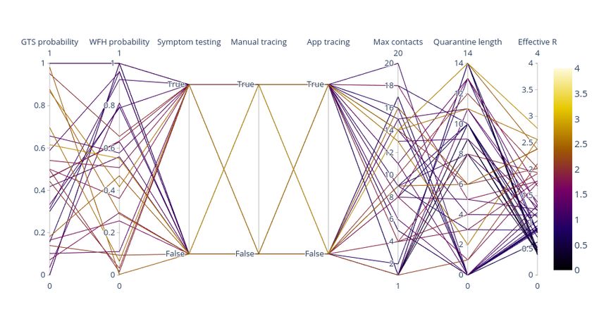
To gain an understanding of how different policy parameters affect the effective R, we plot-
ted the overall search results on a parallel coordinate plot, shown in Figure 14. Generally, we
observed that policies with lower effective R tend to enforce longer quarantine length, limit the
number of contacts, and advocate a work from home policy. We also plotted the overall search
results of isolation decision-related variables, showing that isolating individuals as soon as they
develop symptoms should be advocated for, rather than waiting for positive test results (Figure
15).
20Machine Learning and the Physical World – Group Project
Figure 14: Policy parameter search results on the effective R. Each line in the plots represents a single policy
configuration.
Figure 15: Isolation decision-related variables search results on the effective R. Each line in the plots represents a
single configuration. The columns are variables in the order presented in Table 2
4.2 Ablation Studies
This section discusses ablation test results on both the choice of acquisition functions and sur-
rogate models for the Bayesian optimisation routines.
21Machine Learning and the Physical World – Group Project
Acquisition functions To investigate how different acquisition functions perform we selected
three of them, namely the EI, the negative lower confidence bound (NLCB), and the probability
of improvement (PI). The definition of each function is as follows:
• Expected improvement: the EI [10], computes for each data point, how much it can
improve with respect to the current best observed location f (x∗). Then, it computes the
following equation:
E p( f |D) [max( f (x∗) − f (x), 0)].
where f (x∗) ∈ arg min{ f (x0 ), . . . , f (xn )}. Assuming p( f |D) to be a Gaussian, we can
compute EI in closed form by:
σ (x)(γ(x)Φ(γ(x))) + φ (γ(x))
where γ(x) = f (x?)−µ(x)
σ (x) , Φ is the cumulative distribution function (CDF), and φ is the
probability density function (PDF) of a standard normal distribution.
• Negative lower confidence bound: Based on the upper confidence bound bandit strategy,
the NLCB [25] maximised the following equation:
aLCB = −(µ(x) − β σ (x))
where β is a user-defined hyperparameter that controls exploitation and exploration.
• Probability of improvement: Finally, the PI [10] selects a data point with the highest
probability of improvement over the current best observed location f (x∗), following the
equation:
aPI (x) = Φ(γ(x))
f (x∗)−µ(x)
where γ(x) = σ (x) and Φ is the CDF of a standard normal distribution.
Figure 16(a) illustrates the behaviour of different acquisition functions over iterations. Gen-
erally, all three acquisition functions converged and obtained similar minima. The choice of
acquisition function did not have a large impact on the convergence of the optimisation routine.
Surrogate models We conducted an ablation study on the choice of surrogate models for the
Bayesian optimisation routine. We chose two different models to test, the Gaussian process
and random forest. Each model was tested similarly, with 50 epochs, 10 random initial data
points, and EI as the acquisition function. The result is shown in Figure 16(b), demonstrating
the superiority of the Gaussian process over random forest as a surrogate model.
22Machine Learning and the Physical World – Group Project
(a) Acquisition functions (b) Surrogate models
Figure 16: Left: The effective R across iterations for Bayesian optimisation with different acquisition functions.
Right: The effective R across iterations for Bayesian optimisation with different surrogate models.
4.3 Constrained Optimisation
The constrained optimisation problem aims to find the best set of parameters to minimise the
infection spread, with constraints, such as the number of tests and manual traces [7] reflecting
real-world resource contraints.
Correctly estimating the trade-off between saving lives and minimising disruption lies out-
side the scope of this report. Therefore, we describe two parameterized methods for taking
constraints into account, which can be tuned for practical use based on further research.
The first method is to constrain directly the sampled space, which we did by limiting the
number of testing kits used per day, with the results shown in Table 5. This set of policy
parameters yields an effective R of 0.56 with 0 testing kits. Intuitively, this policy suggests to
not test anyone, and instead enforce everyone to stay at home. This is because, while we have
limited the number of tests, we have not placed any limitations on social distancing or working
from home. To make this approach more practical, it is necessary to add a limit for each of
these measures.
Policy Parameter Optimal Value
go_to_school_prob 0.0166
wfh_prob 0.996
isolate_individual_on_symptoms True
isolate_individual_on_positive True
isolate_household_on_symptoms True
isolate_household_on_positive False
isolate_contacts_on_symptoms False
isolate_contacts_on_positive False
test_contacts_on_positive True
do_symptom_testing False
do_manual_tracing False
do_app_tracing False
23Machine Learning and the Physical World – Group Project
max_contacts 2
quarantine_length 2
Table 5: Set of optimal policy parameters found by Bayesian optimisation, constrained on the number of testing
kits limited to 25k per day.
The second method consists of constructing a different loss function by combining the orig-
inal objective function with penalty terms. We used a linear combination of effective R and all
quantities that increase cost or disruption.
L(x) = λ1 R + λ2 T + λ3 M
where L(x) represents the total loss function arising from the set of policy parameters x, R is
the effective R, T is the number of tests, and M is the number of manual traces. λ1 , λ2 , and λ3
are weights, which we empirically set as λ1 = 0.6, λ2 = 0.2, and λ3 = 0.2. Intuitively, we aim
to minimise the effective R as much as possible, while considering the available resources – the
number of tests and manual traces.
The resulting optimal policy parameters are shown in Table 11. The minimum effective R
found was 1.19. This optimal policy corresponds to 0 manual traces, but 90, 000 tests a day.
This policy seems to be rather lax, as it only requires 80% of the population to work from home
and students are required to attend school. Compared to the policy found by strictly constraining
the number of test kits per day, it seems that this policy might be better, as it demonstrates the
possibility to achieve a lower effective R with a lower number of test kits per day.
5 Conclusion
This report presents the results of comprehensive sensitivity analyses that investigate the effects
of various TTI strategies and NPIs factors on the effective R of COVID-19. On the bases of
these insights, optimisation methods were conducted to find optimal policies that can be used
to help policymakers contain the pandemic. Overall, sensitivity analyses, using axis and grid
variations, and ANOVA decomposition found that work from home, maximum contacts, and
quarantine length factors had the greatest impact on the effective R. Further causal analysis
indicated that these factors indeed directly influence the metric, suggesting that controlling
these factors is key to containing the outbreak. From a technical perspective, we observed the
benefits of employing the Gaussian process emulator, which enabled the fast computation of
ANOVA decomposition, thus allowing the presentation of a more complete sensitivity analysis
result that complement prior work in the COVID-19 domain.
In addition to analysing the effect of various variables on the effective R, we conducted
policy optimisation by using random search, unconstrained Bayesian optimisation, and con-
strained Bayesian optimisation to search for sensible optimal policies. We observed that the
optimal policies derived from all methods agreed with the sensitivity analysis results; that is
they include a strict working from home routine, limit the number of social contacts, and ad-
vocate for long quarantine lengths. While these measures may sound draconian, we have seen
that they effectively reduce the effective R. We also demonstrated the superiority of Bayesian
optimisation-based approaches over the random search, as they obtain better and more sensible
policy significantly faster.
24Machine Learning and the Physical World – Group Project
6 Appendices
Variables
Description
Probability that a person is under 18.
A person that is under 18 has a very
p_under18 different social profile to a person over 18.
A person under 18 is likely to be in school,
General Factors
and a person over 18 is likely to be a working adult.
Probability that home contact is infected,
given that the current individual is infected
home_sar
and interacts with the home contact
(e.g. family members).
Probability that work associate is infected,
work_sar given that the current individual is infected
and interacts with the work associate.
Probability that a person other than work associate
or home family members is infected,
other_sar
given that the current individual is infected and
interacts with that person.
wfh_prob Proportion of people working from home.
Proportion of school-aged children
go_to_school_prob
not going into schools.
Policy Factors A hard limit placed on the number of non-home,
max_contacts
non-work contacts a person has per day.
How long someone has to quarantine
quarantine_length
if they have COVID-19.
testing_delay Delay between test and result (in days).
Delay between a test result and
manual_trace_delay
notifying contacts manually (in days).
Delay between a test result and
app_trace_delay
notifying contacts via app (in days).
Probability that each person complies
with the regulations set out in the policy,
compliance
Compliance Factors such as work from home, quarantine,
and limit social contact.
Percentage of a population using the app
app_cov
to track and trace, and submitting locations.
Table 6: Descriptions of each factor in the groupings discussed in Section 2.
25Variables Description Type
go_to_school_prob Fraction of school children attending school. Float, range:[0,1]
wfh_prob Proportion of the population working from home. Float, range:[0,1]
Isolate the individual after they
isolate_individual_on_symptoms Boolean, range: [True, False]
present with symptoms.
Isolate the individual after they
isolate_individual_on_positive Boolean, range: [True, False]
test positive.
Isolate the household after individual
isolate_household_on_symptoms Boolean, range: [True, False]
present with symptoms.
Isolate the household after individual
isolate_household_on_positive Boolean, range: [True, False]
test positive.
Isolate the contacts after individual presents
isolate_contacts_on_symptoms Boolean, range: [True, False]
with symptoms.
Isolate the contacts after an individual tests
isolate_contacts_on_positive Boolean, range: [True, False]
positive.
Test contacts of a positive case immediately,
test_contacts_on_positive Boolean, range: [True, False]
or wait for them to develop symptoms.
do_symptom_testing Test symptomatic individuals. Boolean, range: [True, False]
do_manual_tracing Perform manual tracing of contacts. Boolean, range: [True, False]
do_app_tracing Perform app tracing of contacts. Boolean, range: [True, False]
max_contacts Limit on the number of contacts per day. Integer, range: [1,20]
Length of quarantine imposed on COVID cases
quarantine_length Integer, range: [0,14]
(and household).
Table 7: Policy optimisation variables, their descriptions and types.GTS WFH Symptom Manual App Max Quarantine
IIS IIP IHS IHP ICS ICP TCP Effective R
Probability Probability Testing Tracing Tracing Contacts Length
0.440 0.830 True True True True False False True False True False 1.0 7.0 0.767
0.146 0.842 True True False True False False False False False True 2.0 3.0 0.771
0.295 0.644 True False False True False True True False False True 3.0 3.0 1.044
0.779 0.331 False True True True True False False True True False 17.0 2.0 1.739
0.288 0.453 False False False False True True True False True True 20.0 13.0 1.921
Table 8: Five selected policy parameters obtained by random search. The columns are variables in the order go to school prob, wfh prob, iso-
late individual on symptoms, isolate individual on positive, isolate household on symptoms, isolate household on positive, isolate contacts on symptoms, iso-
late individual on positive, do symptoms testing, do manual tracing, do app tracing, max contacts, quarantine length, and effective R.
GTS WFH Symptom Manual App Max Quarantine Effective
IIS IIP IHS IHP ICS ICP TCP
Probability Probability Testing Tracing Tracing Contacts Length R
0.0 1.0 True True True False True False True False True True 1.0 14.0 0.383
0.0 1.0 True True True True True True False True True False 1.0 8.0 0.44
0.0 1.0 True False False False True True True True True True 9.0 10.0 0.838
0.0 1.0 True True True False False False True True False True 20.0 0.0 1.027
0.165 0.256 True True False True False False False False False False 8.0 13.0 1.68
Table 9: Five selected policy parameters obtained by unconstrained Bayesian optimisation. The columns are variables in the order go to school prob, wfh prob,
isolate individual on symptoms, isolate individual on positive, isolate household on symptoms, isolate household on positive, isolate contacts on symptoms, iso-
late individual on positive, do symptoms testing, do manual tracing, do app tracing, max contacts, quarantine length, and effective R.GTS WFH Symptom Manual App Max Quarantine Days
IIS IIP IHS IHP ICS ICP TCP
Probability Probability Testing Tracing Tracing Contacts Length Quarantined
0.264 0.095 False False False True False False True False False False 15.0 0.0 0.000
0.278 0.338 False False False True False False True False False True 14.0 3.0 51.048
0.926 0.992 False True False True False False False True False True 20.0 2.0 53.112
0.247 0.477 False True False False False True True True False True 20.0 2.0 68.496
0.144 0.401 False False False True True True False False False False 6.0 6.0 110.088
Table 10: Five selected policy parameters obtained by unconstrained Bayesian optimisation optimising on person days quarantined. The columns are variables in
the order go to school prob, wfh prob, isolate individual on symptoms, isolate individual on positive, isolate household on symptoms, isolate household on positive,
isolate contacts on symptoms, isolate individual on positive, do symptoms testing, do manual tracing, do app tracing, max contacts, quarantine length, and person
days quarantined (in thousands).
GTS WFH Symptom Manual App Max Quarantine Weighted Effective
IIS IIP IHS IHP ICS ICP TCP
Probability Probability Testing Tracing Tracing Contacts Length Combination R
1.0 0.8 True False True False False False False False False True 1.0 14.0 1.154 1.187
1.0 0.8 True False True False False False False False False True 1.0 14.0 0.718 1.197
1.0 0.8 True False True False False False False False False True 1.0 14.0 1.055 1.508
0.279 0.154 False True False False True True True True False True 7.0 7.0 1.17 1.702
0.945 0.671 True True False True False True True True False True 9.0 8.0 1.424 2.127
Table 11: Five selected policy parameters obtained by constrained Bayesian optimisation optimising the weighted loss function. The columns are variables in the
order go to school prob, wfh prob, isolate individual on symptoms, isolate individual on positive, isolate household on symptoms, isolate household on positive, iso-
late contacts on symptoms, isolate individual on positive, do symptoms testing, do manual tracing, do app tracing, max contacts, quarantine length, weighted combi-
nation, and effective R.Machine Learning and the Physical World – Group Project
References
[1] Abel Brodeur, David M Gray, Anik Islam, and Suraiya Bhuiyan. A literature review of
the economics of covid-19. 2020.
[2] Veronica Czitrom. One-factor-at-a-time versus designed experiments. The American
Statistician, 53(2):126–131, 1999.
[3] Nicholas G Davies, Adam J Kucharski, Rosalind M Eggo, Amy Gimma, W John Ed-
munds, Thibaut Jombart, Kathleen O’Reilly, Akira Endo, Joel Hellewell, Emily S Nightin-
gale, et al. Effects of non-pharmaceutical interventions on covid-19 cases, deaths, and
demand for hospital services in the uk: a modelling study. The Lancet Public Health,
2020.
[4] Jonathan I Dingel and Brent Neiman. How many jobs can be done at home? Technical
report, National Bureau of Economic Research, 2020.
[5] GPy. GPy: A gaussian process framework in python. http://github.com/
SheffieldML/GPy, since 2012.
[6] Yan Guo, Chao Cheng, Yu Zeng, Yiran Li, Mengting Zhu, Weixiong Yang, He Xu, Xiao-
hua Li, Jinhang Leng, Aliza Monroe-Wise, et al. Mental health disorders and associated
risk factors in quarantined adults during the covid-19 outbreak in china: cross-sectional
study. Journal of medical Internet research, 22(8):e20328, 2020.
[7] Josh Halliday. Coronavirus home test kits ’run out’ in england and scotland, 2020.
[8] Agus Hasan, Hadi Susanto, Muhammad Firmansyah Kasim, Nuning Nuraini, Bony
Lestari, Dessy Triany, and Widyastuti Widyastuti. Superspreading in early transmissions
of covid-19 in indonesia. Scientific reports, 10(1):1–4, 2020.
[9] Bobby He, Sheheryar Zaidi, Bryn Elesedy, Michael Hutchinson, Andrei Paleyes, Guy
Harling, Anne Johnson, and Yee Whye Teh. Technical document 3: Effectiveness and
resource requirements of test, trace and isolate strategies. 2020.
[10] Donald Jones, Matthias Schonlau, and William Welch. Efficient global optimization of
expensive black-box functions. Journal of Global Optimization, 13:455–492, 12 1998.
[11] Petra Klepac, Stephen Kissler, and Julia Gog. Contagion! the bbc four pandemic–the
model behind the documentary. Epidemics, 24:49–59, 2018.
[12] Adam J Kucharski, Petra Klepac, Andrew Conlan, Stephen M Kissler, Maria Tang, Han-
nah Fry, Julia Gog, John Edmunds, CMMID COVID-19 Working Group, et al. Effective-
ness of isolation, testing, contact tracing and physical distancing on reducing transmission
of sars-cov-2 in different settings. medRxiv, 2020.
[13] Jia Jia Liu, Yanping Bao, Xiaolin Huang, Jie Shi, and Lin Lu. Mental health considerations
for children quarantined because of covid-19. The Lancet Child & Adolescent Health,
4(5):347–349, 2020.
[14] Elisabeth Mahase. Covid-19: What is the r number? BMJ, 369, 2020.
29Machine Learning and the Physical World – Group Project
[15] Amandine Marrel, Bertrand Iooss, Beatrice Laurent, and Olivier Roustant. Calculations
of sobol indices for the gaussian process metamodel. Reliability Engineering & System
Safety, 94(3):742–751, 2009.
[16] Frank J Massey Jr. The kolmogorov-smirnov test for goodness of fit. Journal of the
American statistical Association, 46(253):68–78, 1951.
[17] James M Murphy, David MH Sexton, David N Barnett, Gareth S Jones, Mark J Webb,
Matthew Collins, and David A Stainforth. Quantification of modelling uncertainties in a
large ensemble of climate change simulations. Nature, 430(7001):768–772, 2004.
[18] Hiroshi Nishiura, Tetsuro Kobayashi, Takeshi Miyama, Ayako Suzuki, Sung-mok Jung,
Katsuma Hayashi, Ryo Kinoshita, Yichi Yang, Baoyin Yuan, Andrei R Akhmetzhanov,
et al. Estimation of the asymptomatic ratio of novel coronavirus infections (covid-19).
International journal of infectious diseases, 94:154, 2020.
[19] World Health Organization et al. Protocol for assessment of potential risk factors for
coronavirus disease 2019 (covid-19) among health workers in a health care setting, 23
march 2020. Technical report, World Health Organization, 2020.
[20] Andrei Paleyes, Mark Pullin, Maren Mahsereci, Neil Lawrence, and Javier González. Em-
ulation of physical processes with emukit. In Second Workshop on Machine Learning and
the Physical Sciences, NeurIPS, 2019.
[21] Judea Pearl and Dana Mackenzie. The book of why: the new science of cause and effect.
Basic Books, 2018.
[22] B. Shahriari, K. Swersky, Z. Wang, R. P. Adams, and N. de Freitas. Taking the human out
of the loop: A review of bayesian optimization. Proceedings of the IEEE, 104(1):148–175,
2016.
[23] Ilya M Sobol. Global sensitivity indices for nonlinear mathematical models and their
monte carlo estimates. Mathematics and computers in simulation, 55(1-3):271–280, 2001.
[24] Il’ya Meerovich Sobol’. On sensitivity estimation for nonlinear mathematical models.
Matematicheskoe modelirovanie, 2(1):112–118, 1990.
[25] Niranjan Srinivas, Andreas Krause, Sham M Kakade, and Matthias Seeger. Gaussian
process optimization in the bandit setting: No regret and experimental design. arXiv
preprint arXiv:0912.3995, 2009.
[26] Fang Tang, Jing Liang, Hai Zhang, Mohammedhamid Mohammedosman Kelifa, Qiqiang
He, and Peigang Wang. Covid-19 related depression and anxiety among quarantined re-
spondents. Psychology & health, pages 1–15, 2020.
[27] The DELVE Initiative. Test, trace, isolate. Technical report, 2020.
30You can also read