Adversarial Active Learning for Sequence Labeling and Generation - IJCAI
←
→
Page content transcription
If your browser does not render page correctly, please read the page content below
Proceedings of the Twenty-Seventh International Joint Conference on Artificial Intelligence (IJCAI-18)

           Adversarial Active Learning for Sequence Labeling and Generation

                         Yue Deng1 , KaWai Chen2 , Yilin Shen1 , Hongxia Jin1
                      1
                    AI Center, Samsung Research America, Mountain View, CA, USA
        2
          Department of Electrical and Computer Engineering, University of California, San Diego
                {y1.deng, yilin.shen, hongxia.jin}@samsung.com, w0chen@eng.ucsd.edu

                          Abstract                                      certainty measures can be defined from various perspectives
                                                                        including probabilistic confidence [Culotta and McCallum,
     We introduce an active learning framework for gen-                 2005], margin value [Scheffer et al., 2001], entropy [Deng et
     eral sequence learning tasks including sequence la-                al., 2016], fisher information [Sutton and McCallum, 2006;
     beling and generation. Most existing active learn-                 Bao et al., 2017] and a score voted by several base mod-
     ing algorithms mainly rely on an uncertainty mea-                  els [Seung et al., 1992; Deng et al., 2017b]. While these
     sure derived from the probabilistic classifier for                 active learning algorithms work well for data classification
     query sample selection. However, such approaches                   tasks, they are unfortunately not easily extended to solving
     suffer from two shortcomings in the context of se-                 sequence learning problems due to the complexity of the la-
     quence learning including 1) cold start problem and                bel space. Consider a label sequence with p tokens and each
     2) label sampling dilemma. To overcome these                       token can belong to k possible classes, then there are k p pos-
     shortcomings, we propose a deep-learning-based                     sible combinations of the label sequence. This complexity
     active learning framework to directly identify query               can grow exponentially with the length of the output.
     samples from the perspective of adversarial learn-
     ing. Our approach intends to offer labeling prior-                    We consider two major challenges faced by existing active
     ities for sequences whose information content are                  learning approaches in handling sequence learning tasks: 1)
     least covered by existing labeled data. We ver-                    cold start problem and 2) label-sampling dilemma. The first
     ify our sequence-based active learning approach                    cold-start challenge is mainly due to the complexity of the
     on two tasks including sequence labeling and se-                   learning system for structured prediction. Unlike classifica-
     quence generation.                                                 tion tasks that just need a simple probabilistic classifier, the
                                                                        predictor for sequences are configured within a complex re-
                                                                        current structure, e.g. a LSTM. Training a structured predic-
1   Introduction                                                        tor with very limited labeled sequence can easily lead to a bi-
Active learning (AL) is a traditional approach to solve su-             ased estimation. If the predictor itself is seriously biased, how
pervised learning problems without sufficient labels. While             can we trust the uncertain measure derived from it? This cold
there have been many existing AL works proposed for clas-               start problem easily happens during the initial steps of active
sification problems [Settles, 2010; Scheffer et al., 2001;              learning when there are only insufficient labeled samples in
Deng et al., 2013], active learning algorithms for sequences            hand. The second label sampling dilemma is ascribed to the
are still not widely discussed. With the growing interests in           inability of the full enumeration of all possible sequence la-
AI research, many newly emerged problems are exactly de-                bels. In detail, when calculating an uncertainty score e.g.,
fined in the scope of sequence learning including image cap-            the entropy, for a sequence, all possible label combinations
tioning [Vinyals et al., 2015], machine translation [Luong et           should be taken into account (see Eq. 3) that can become
al., ] and natural language understanding [Dong and Lapata,             impossible when the output sequences are too long. There-
2016]. Compared with classification tasks that only need one            fore, only approximated uncertainty measures can be used as
label for a sample, sequence learning tasks require a series            a surrogate for sequence-based active learning.
of token-level labels for a whole sequence. Precise annota-                To overcome the aforementioned limitations, we propose
tions for sequences are not only labor-consuming but may                a new active learning framework for sequences inspired by
also require very specific domain knowledge [Dong and Lap-              adversarial learning. Our approach alleviates the demands
ata, 2016] that are not easily accomplished by crowd-sourcing           on the structured predictor for query sample selection. The
workers. This apparent difficulty in sequence labeling exactly          proposed adversarial active learning framework incorporates
motivates our explorations of more effective active learning            a neural network to explicitly assert each sample’s informa-
approaches for sequences.                                               tiveness with regard to labeled data. The easily-induced ac-
   Existing active learning strategies mainly rely on some un-          tive score avoids heavy computations in sampling the whole
certainty measures derived from a classifier for query sam-             label space and can improve the active learning efficiency by
ple selection [Cohn et al., 1994; Settles, 2010]. These un-             more than 100 times on some large datasets.

                                                                 4012
Proceedings of the Twenty-Seventh International Joint Conference on Artificial Intelligence (IJCAI-18)
2 Preliminaries sample, where xL is the input data that can be of any type
2.1 Active Learning for Sequences including images, speeches and texts depending on different
learning tasks; and y L is the targeted output sequence com-
In this part, we review some existing active learning ap- posed of p tokens y L = {y1L ...ypL }. A feature encoder M ()
proaches for sequence learning [Settles and Craven, 2008].
is established to map the input xL to a latent representation
The first widely used uncertainty measure defined from the
z L = M (xL ). M () can be a convolution neural network for
probabilistic classifier is the least confidence (LC) score:
image data or a recurrent neural network for speeches and
ψLC (xU ) = 1 − P (y ∗ |xU ), (1) texts. Then, a decoder C() adopts z L as a conditional input
∗ U
and sequentially predicts each token in y P :
where y is the most likely label sequence and x is an unla-
beled sample. While this measure is intuitive, the calculation P (y p = {y1P ...yqP }|x)
of the most likely label sequence is not easy. It requires the T (5)
= P (y1p |z L = M (xL )) p
P (ytp |y1p ...yt−1 , z L ),
Q
dynamic programming to find the Viterbi parse. Similarly, t=1
the margin term can also be used to define the uncertainty for
an unknown sample: The above generative probability can be well modeled by a
recurrent neural network, e.g., a LSTM [Deng et al., 2017a].
ψM (xU ) = P ((y2∗ |xU )), −P (y1∗ |xU ), (2) The encoded latent representation z L is used as the ‘start-
ing key’ at step zero. Then, it sequentially outputs each to-
where y1∗ and y2∗ are the first and second best label sequences,
ken yt based on the tth step’s input and the memory vector
respectively.
maintained by the recurrent neural network [Sutskever et al.,
The sequence entropy term is also widely used as an un-
2014]. The training loss of this sequence learning part is ob-
certainty score [Settles and Craven, 2008]:
tained by counting the differences between the predicted se-
quence y P and the ground truth labels y L :
X
ψEN (xU ) = − P (y p |xU ) log P (y p |xU ) (3)
yp Ls (X L , Y L ) = L(y L , y P )
P
L L L L
(6)
where y p ranges over all possible label sequences for input (x ,y )∼(X ,Y )
xU . We have also noted that the number of possible labeling We noted that both y L is the labeled sequence; and predicted
grows exponentially with the desired output sequence length. sequence y P is generated by a function of xL (see Eq.5) ; L
For the ease of computation, we follow previous work to em- can be arbitrary losses defined over two sequences such as the
ploy an approximated N-best sequence entropy (NSE) [Kim prevalent cross-entropy. Here, we just briefly introduced this
et al., 2006], encoder-decoder framework and interested readers are refer-
eed to [Sutskever et al., 2014; Xu et al., 2015] for details.
X
ψN SE (xU ) = − P (y p |xU ) log P (y p |xU ) (4)
y p ∈N
3 Adversarial Active Learning for Sequences
N = {(y 1 )p , ..., (y N )p } corresponds to N most likely parses.
3.1 ALISE Model
These N most likely parses can obtained through beam search
[Koehn, 2004]. The labeling priority should be given to sam- It is conceivable that sequence learning model requires a huge
ples with high entropy (corresponding to low confidence). amount of labeled data for robust training. We hence consider
While the definition of these terms are different, they are all developing an active learning algorithm to facilitate the whole
closely related to the structured predictor. The calculations of labeling process. In our approach, we consider defining an ac-
these uncertainty scores are also not trivial and may require tive score based on the informativeness of an unlabeled sam-
some algorithmic explorations such as the dynamic program- ple xU with respect to all labeled samples X L :
ming or the beam search. When the candidate samples’ quan-
s(xU ) = sim(xU , X L ) (7)
tity is large, the calculation of such complexity uncertainty
measures can take a quite long while in scoring all individual where X L is the set containing all labeled samples and
samples from the data pool. These obvious shortcomings mo- sim(·, ·) defines a similarity score between a point xU and
tivate us to design more efficient and advanced active learn- a training set X L composed of labeled samples. The score in
ing strategies for sequence learning. In this work, we propose Eq.7 helps to rank unlabeled samples based on their inherent
such a desired framework from adversarial learning [Deng et informativeness similarity to existing labeled data. A small
al., 2017c]. The active learning strategy in our model is not similarity score implies the certain unlabeled sample is not
related to the structured output predictor and hence can con- related to any labeled samples in training set and vice versa.
duct query samples scoring in light on very large dataset. The labeling priority is offered to samples with low similarity
scores.
2.2 Encoder-decoder Framework We take image captioning as an intuitive instance to ex-
Before going to the details about our active learning model, plain the rational behind our active scoring approach. In the
we will first review the prevalent encoder-decoder framework training set, most images and their corresponding descrip-
for sequence learning. This generic encoder-decoder model tions are about human sports such as skating, running and
serves as the basic building block of our active learning sys- swimming. Then, we have access to two extra unlabeled im-
tem. We denote (xL , y L ) ∼ (X L , Y L ) as a pair of labeled ages that are respectively related to “swimming” and “a plate
4013Proceedings of the Twenty-Seventh International Joint Conference on Artificial Intelligence (IJCAI-18)
M () intends to fool the discriminator to regard all latent rep-
resentations (z L and z U ) as already labeled. Mathematically,
it encourages the discriminator D to output a score 1 for both
z L and z U . The corresponding loss is modeled by the cross-
entropy in the first two terms of the following equation:
min LM = −ExL ∼X L [(log D(M (xL )]
(8)
−ExU ∼X U [log D(M (xU ))] + λLs (X L , Y L ),
In addition to the cross-entropy loss defined on the discrimi-
nator side, the above equation also takes the supervised loss
Figure 1: An overview of Adversarial Active Learning for sequences in Eq.6 into consideration, i.e., in the third term. In all, the
(ALISE). The black and blue arrows respectively indicate flows for learning objectives of the feature encoder M are concluded
labeled and unlabeled samples. as two-fold: 1) fool the discriminator and 2) improve the fit-
. ting quality on labeled data. These two learning objectives
are balanced by a hyper-parameter λ.
of food”. With those annotated images in hand, which unla- The learning objective of the discriminator D goes against
beled image should be labeled first? There is no doubt that to the objective in Eq. 8. The discriminator is trained to cor-
the image about ‘food’ should be sent out for captioning by rectly assign z L = M (xL ) to labeled category (D(Z L ) = 1)
human. This is because there are already some swimming and z U = M (xU ) to unlabeled class (D(Z U ) = 0). The
images in the existing training pool and adding another sim- corresponding learning objective of D is also defined by the
ilar image may not offer too much ‘new’ knowledge to the cross-entropy:
learning system. On the contrary, the image about food is
min LD = −ExL ∼X L [(log D(M (xL )]
not covered in existing training set and its captions can bring (9)
more valuable complementary information. −ExU ∼X U [log(1 − D(M (xU )))]
However, the problem still remains in how to quantitatively This adversarial discriminator D exactly serves the pur-
evaluate the informativeness similarity between an unlabeled pose of distribution comparisons between two set of sam-
sample with the labeled data pool. For sequence data, the sim- ples. In GAN work [Deng et al., 2017c], it is indicated that
ilarity calculation itself is a difficult problem due to the vari- the adversarial discriminator implicitly compares the gener-
ations in sequence lengths. Existing approaches mainly play ative distributions between real data and fake data. Here,
kernel tricks to map the original sequences into a kernel space we borrowed the same adversarial learning idea to compare
with fixed-length feature representations [Settles and Craven, the distributions between labeled and unlabeled samples. In
2008]. However, the selection of an appropriate kernel re- GAN (resp. our ALISE model), the discriminator outputs
quires sophisticated domain knowledge and the best kernel low scores for those fake (resp. unlabeled) samples that are
can vary from task to task. For instance, the best kernels for mostly not similar to real images (resp. labeled data). There-
Chinese and French sentences are obviously not the same. fore, the score from this discriminator already serves as an
In this work, we propose a new adversarial active learning informativeness similarity score that could be directly used
model for sequences (ALISE). In our ALISE, we consider de- for Eq.7. The feature encoder M , sequence decoder C and
signing a discriminator network D(·) to directly outputs the adversarial discriminator D can all be trained in an alterna-
informativeness similarity scores for unlabeled samples. In tive manner by iteratively optimizing the objectives in Eq.8
Fig. 1, we pass both a labeled sample xL and an unlabeled and Eq.9. We have detailed the learning steps in Algorithm 1.
sample xu trough the same feature encoder M (shared pa-
rameters), then we get z L = M (xL ) (latent representation
3.2 Active Scoring
for labeled data) and z U = M (xU ) (latent representation for After well training, we can pass all unlabeled samples
unlabeled data). These two latent representations are further through M and D to get their corresponding score by ALISE
fed into the discriminator network (D), which is trained to framework, i.e.,
classify whether the certain data is sampled from labeled or
s(xU ) = D(M (xU )) ∈ (0, 1), ∀xU ∈ X U (10)
unlabeled data pool. The output of the D is a sigmoid func-
tion that indicates how likely the certain sample is from the The score s = 1 (resp. s = 0) means the information content
labeled pool. of the certain unlabeled sample is most (resp. least) covered
The learning objectives of M and D are involved in an ad- by the existing labeled data. Apparently, those samples with
versarial process. From the aspect of encoder M , it intends lowest scores should be sent out for labeling because they
to map all data to a latent space where both labeled and unla- carry most valuable information in complementary to the cur-
beled data can follow very similar probabilistic distributions. rent labeled data.
In the most ideal scenario that if z L and z U follow exactly the It is noted that our ALISE approach does not rely on the
same generative probability, then the decoder C trained with structured predictor (i.e. the decoder C) for uncertainty mea-
z L should also seamlessly work on latent representations z U sure calculation. However, we can still consider incorporat-
obtained from unlabeled sample xU . Therefore, the encoder ing existing predictor-dependent uncertainty scores into our
4014Proceedings of the Twenty-Seventh International Joint Conference on Artificial Intelligence (IJCAI-18)
Algorithm 1: ALISE Learning
Input : A data pool composed of labeled and unlabeled
data X = {X L , X U }; X L are paired with
sequence label Y L = {y1L ...ypL };
Initialization: Initialize parameters in encoder network M and
decoder network C by training an
encoder-decoder framework with available
training samples (X L , Y L ); Initialize
parameters in the discriminator network D
randomly.
1 for epoch=1...K do
2 for all mini-batches (xL , y L ) ∼ (X L , Y L ) and xU ∼ X U
do
3 Minimize the loss LM in Eq.8 to update parameters in
the encoder network M and decoder network C
4 Minimize the loss LD in Eq.9 and update parameters
in discriminator network D
5 end
6 end
Output : The well trained M, C and D
Figure 2: Slot filling F-score of different active learning approaches.
.
framework. Because the ALISE framework has already been
built with a probabilistic decoder C(), then the calculations
of uncertainty measures from it is natural and convenient. In same length. This part of experiments were mainly conducted
such a combinational setting, we can first select K top sam- on the ATIS (Airline Travel Information Systems) dataset
ples selected by the adversarial discriminator. Then, within [Hemphill et al., 1990]. We obtained ATIS text corpus that
these K samples, we further calculate their sequence-based was used in [Liu and Lane, 2016] and [Deoras and Sarikaya,
uncertainty scores ψ(xU ) (e.g. the sequence entropy) as in- 2013] for active learning. For instance, an input sentence in
troduced in Section 2.1. The top k samples with highest ATIS xL = {business, class, fare,from, SF, to, LA} can be
uncertainty scores are selected as query samples for label- parsed as a label sequence y L = {B-class-type, I-class-type,
ing. These candidate query samples are mainly determined O, O, B-from-loc, B-to-loc}. This studied dataset contains
by the adversarial discriminator and the probabilistic decoder 5138 utterances with annotated slot labels.
only provides auxiliary information for fine-grained selec- We follow the same implementation in [Liu and Lane,
tion. Moreover, the complexity for sequence-based uncer- 2016] to use a bi-directional LSTM as the encoder network
tainty measure computations have also been reduced. This is M in Fig.1. This bidirectional LSTM read the input sentence
because the uncertainty measure is only required to be com- in both forward and backward directions and their hidden
puted on K candidate samples selected by ALISE rather than states at each step were concatenated as the long vector. We
the whole pool of unlabeled samples. choose 128 for word embedding layer and 64 hidden states
While there are some early works that also use the ‘buz- for the encoder LSTM. To this end, we have obtained 128
zwords’ adversarial active learning, they are totally different dimensions for the latent representation z. The decoder C
from our ALISE. First, the work in [Zhu and Bento, 2017] in Fig.1 is implemented by either a standard LSTM decoder
used the GAN model to generate fake images and then label- [Sutskever et al., 2014] or a more advanced attention model
ing those fake images to augment training set. ALISE does [Liu and Lane, 2016]. Both of them are widely used in ex-
not generate any fake sample and just borrows the adversarial isting literatures. The adversarial network D is configured by
learning objective for sample scoring. The work in [Miller three dense-connected layers with 128 (input layer), 64 (in-
et al., 2014] is totally none related to adversarial learning. It termediate layer) and 1 (output layer) units, respectively. The
just uses traditional active learning approach to solve the ad- output layer is further connected with a sigmoid function for
versarial attract problem in security domain. probabilistic conversion. We use relu activation among all
other layers. Each token of the output sequence is coded as
4 Experiments a one-hot vector with the hot entry indicating the underly-
ing cateogory of the token. The whole deep learning system
In this part, we investigate the performances of ALISE on was trained by ADAM [Kingma and Ba, 2014]. Among all
two sequence learning tasks including slot filling and image labeled training samples, we further randomly select 10% of
captioning. them as validation samples. The whole training process is ter-
minated when the loss on the validation set does not decrease
4.1 Slot Filling or when the optimization reaches 100 epochs.
Slot filling is a basic component of spoken language under- We consider comparing our ALISE approach with existing
standing. It can be viewed as a sequence labeling problem, sequence-based active learning algorithms. The competitors
where both the input and output label sequences are of the include random sampling, least confidence score (see Eq.2),
4015Proceedings of the Twenty-Seventh International Joint Conference on Artificial Intelligence (IJCAI-18)
N-best sequence entropy (NSE, see Eq.4). Moreover, we fur-
ther consider the combinational scoring approach as intro-
duced in Section 3.2 that we combine both ALISE scores and
NSE scores for query sample selection. To make fair com-
parisons, the number of optimal decoding parses (N) is cho-
sen as five for both NSE approach and our ALISE+NSE ap-
proach. In active sequence learning, we randomly select 2130
sequences as testing samples. The remaining 3000 sequences
are used for model training and active labeling.
In detail, among these 3000 data, p = 300 samples are
randomly chosen as initial labeled data. Then, we train the
ALISE model with these p = 300 samples and conduct ac-
tive learning based on the remaining 3000 − p non-testing
samples. k = 300 top samples returned by different active
learning methods are selected for label query. After labeling,
these k samples will be merged with the existing p labeled
samples as the new labeled pool. The ALISE and other ac-
tive learning models will be trained with this new labeled set Figure 3: Image captioning results by active learning.
and the trained model will be used to select another k unla- .
beled samples for the next round. Such query sample selec-
tion, labeling approach and model retraining processes will
be iteratively conducted. We only report results until we have ground truth captions. In our active learning setting, the query
get 2700 training samples because it is the limitation for ac- sample selection is mainly conducted at the image level. It
tive selection. When all 3000 points are used, there are no means that if one image has been selected for labeling, its cor-
distinctions among different active learning algorithms. The responding five ground-truth captions are all accessible. We
active learning results with different training sample sizes are follow Karpathy et al.[Karpathy and Fei-Fei, 2015] to pre-
reported in Fig.2, where both the LSTM and attention model porcess the sentences, where all the words are converted to
are respectively used as the decoder C for sequence label pre- lower-case, and all non-alphanumeric characters are discards.
diction. In the figure, we do the random splitting process for We discarded all words that appear less than twice in all cap-
five times and the average F-score with standard deviations tions.
are reported. Here, we choose the F-score as the accuracy in- We consider all 82,783 training set as the basic data pool
dicator because it is widely used in existing works [Liu and for active learning and query selection. We increase the la-
Lane, 2016][Deoras and Sarikaya, 2013] beled samples’ rate from 0.2 to 0.8 with 0.2 as an incremen-
From the results, we have observed that our ALISE model tal step. Among the first 0.2× 82,783 samples, half of them
and its combinational extension (ALISE+NSE) both outper- are randomly chosen as the initial labeled set and the remain-
form existing sequence learning approaches. When the la- ing are selected by different active learning algorithms. The
beled number size is small, the improvements of two ALISE active selection and learning processes are iteratively con-
models are more significant. The ALISE+NSE model fur- ducted by adding k =0.2× 82,783 new labeled samples to
ther improves the performances of ALISE. However, when the labeled pool in each round. These extra k samples are
the number of sample sizes is relatively large, the differences selected by different active learning algorithms. The perfor-
between ALISE and ALISE+NSE are minor. However, these mances of ALISE are compared with other active learning
two ALISE methods are still better than other sequence learn- approaches in Fig.3. For result evaluations, we follow exist-
ing approaches. Meanwhile, we have observed that using at- ing works to report BLEU-4 and METEOR as the accuracy
tention model as the sequence decoder is much better than the indicator. These two accuracy measures can be easily calcu-
LSTM model. lated by the MSCOCO API. We repeat the aforementioned
active learning process for 5 times with average and standard
4.2 Image Captioning deviation reported in Fig.3. We have observed from quanti-
We further apply ALISE model for the sequence generation tative evaluation that ALISE models (the original ALISE and
task of image captioning. In this task, the input data is an im- ALISE+NSE) beat all existing active learning models based
age and the corresponding label is a caption sentence describ- on these two scores. Meanwhile, the performance of ALISE
ing the content of the input image. We follow the same con- can be further enhanced by combining NSE score as auxiliary
figuration and parameter settings in the work [Xu et al., 2015] indicator (ALISE+NSE).
to implement the encoder-decoder learning framework. The To better understand differences among various active
structure of the adversarial discriminator in ALISE is kept learning approaches, we provide some captioning results as
the same as in the slot filling experiment. This part of ac- intuitive instances in Fig.4. All these image captioning mod-
tive learning experiments are mainly conducted on MSCOCO els are trained with 80% data points from the training set.
dataset [Lin et al., 2014], which consists of 82,783 images Nevertheless, these same amount of training samples are
for training, 40,504 for validation, and 40,775 for testing. We selected by different active learning methods. In the fig-
noted that each image in MSCOCO dataset is paired with 5 ure, we provide the captioning results by NSE, ALISE and
4016Proceedings of the Twenty-Seventh International Joint Conference on Artificial Intelligence (IJCAI-18)
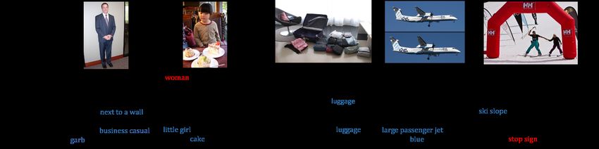
Figure 4: Image captioning results in the active learning setting by ALISE, ALISE+NSE and NSE-based approaches. The novel plausible
descriptions are annotated with blue color while wrong descriptions are colored in red.
.
ALISE+NSE because these three algorithms outperform oth- Slot Filling Captioning
ers in Fig.3. From these intuitive results, we have observed LC 173s 2182s
that the two ALISE models tends to use more complex sen- NSE 245s 3956 s
tence structures for image descriptions. Moreover, these two
ALISE models can cover more details about the visual infor- ALISE 1.7s 6.9 s
mation. It is mainly because the ALISE approach can ac- ALISE+NSE 11.3s 67.4 s
tively build up a training set covering diverse information.
However, there is still small chance that the ALISE model Table 1: The active selection costs for different algorithms
over-explains the image with wrongly recognized objects.
As shown in the rightest sub-figure in Fig.4, ALISE+NSE
model mistakenly describes the red finishing line as a stop and image captioning datasets, respectively. The correspond-
sign. However, the captioning results of ALISE model are ing costs of different algorithms are reported in ??. Here, we
still much better than the NSE approach in producing precise omit the complexity of random sampling because it can be
captioning sentences in a more natural manner. finished in real time.
We have found that ALISE methods are much faster than
4.3 Computational Complexity existing sequence-based active learning approaches. This is
because the calculation of the LC and NSE scores require the
We also reported the computational costs of ALISE. We have Viterbi parsing and beam search over the whole output space.
observed that the computational costs of ALISE are almost Therefore, their costs are significant higher when the sam-
the same as the original baseline model. In detail, we respec- ple size is large (as in the image captioning dataset). How-
tively report the training costs on the slot filling and image ever, the scoring mechanism in ALISE method just requires
captioning tasks for references. The ALISE training in slot passing all samples through a trained neural network (i.e. the
filling task (with 2700 samples) can be accomplished in just adversarial discriminator D in Fig.1). Therefore, the corre-
74 seconds with 16 GPUs (Tesla K80) parallelized in opti- sponding active scoring cost can be minor. The ALISE+NSE
mization. The original Attention-based encoder-decoder slot- can also be efficiently implemented because it just performs
filling model costs 53 seconds when trained with the same N-best sequence entropy calculations on a selected number
amount of data [Liu and Lane, 2016]. For the image cap- of samples filtered by ALISE model. Therefore, its computa-
tioning task, the baseline attention model [Xu et al., 2015] tional costs are a bit higher than ALISE but are still far more
and ALISE respectively spends an average of 2.7 hours and less than other approaches.
3.2 hours in total on 66,000 images. From these two tasks,
the training cost of ALISE is not that different than the cor-
responding baseline encoder-decoder model. This is because 5 Discussions
ALISE has only introduced an auxiliary adversarial discrim- We introduced a sequence-based active learning model
inator in the model and this discriminator neural network ex- ALISE from the perspective of adversarial learning. It con-
hibits very simple structures (just a multi-layer neural net- ducts query sample selections based on a well trained dis-
work with a 64 nodes intermediate layer and a 1 node output criminator. Therefore, ALISE is much more efficient than ex-
layer.). isting predictor-dependent active learning approaches. More-
However, the active learning complexity of different meth- over, our model accomplishes both the tasks of active learn-
ods can vary significantly, especially when the candidate un- ing and sequence learning into a joint framework that is end-
labeled pool size is large. We report the query sample selec- to-end trainable. Therefore, it is seamlessly applied to di-
tion costs on the aforementioned two datasets, that include verse learning tasks across different domains. Experimental
2,400 (i.e., the first data point in Fig.2) and 66,000 ( i.e., the verifications show that ALISE can greatly improve the per-
first data point in Fig.3) candidate samples on the slot filling formances and speed of existing models in the early active
4017Proceedings of the Twenty-Seventh International Joint Conference on Artificial Intelligence (IJCAI-18)
learning stages with insufficient training samples. [Koehn, 2004] Philipp Koehn. Pharaoh: a beam search
decoder for phrase-based statistical machine translation
References models. In Association for Machine Translation in the
[Bao et al., 2017] Feng Bao, Yue Deng, Mulong Du, Zhi- Americas, pages 115–124. Springer, 2004.
quan Ren, Qingzhao Zhang, Yanyu Zhao, Jinli Suo, [Lin et al., 2014] Tsung-Yi Lin, Michael Maire, Serge Be-
Zhengdong Zhang, Meilin Wang, and Qionghai Dai. Prob- longie, James Hays, Pietro Perona, Deva Ramanan, Pi-
abilistic natural mapping of gene-level tests for genome- otr Dollár, and C Lawrence Zitnick. Microsoft coco:
wide association studies. Briefings in bioinformatics, page Common objects in context. In ECCV, pages 740–755.
bbx002, 2017. Springer, 2014.
[Cohn et al., 1994] David Cohn, Les Atlas, and Richard Lad- [Liu and Lane, 2016] Bing Liu and Ian Lane. Attention-
ner. Improving generalization with active learning. Ma- based recurrent neural network models for joint intent de-
chine learning, 15(2):201–221, 1994. tection and slot filling. Interspeech, 2016.
[Culotta and McCallum, 2005] Aron Culotta and Andrew [Luong et al., ] Minh-Thang Luong, Hieu Pham, and
McCallum. Reducing labeling effort for structured pre- Christopher D Manning. Effective approaches to
diction tasks. In AAAI, volume 5, pages 746–751, 2005. attention-based neural machine translation.
[Deng et al., 2013] Yue Deng, Qionghai Dai, Risheng Liu, [Miller et al., 2014] Brad Miller, Alex Kantchelian, Sadia
Zengke Zhang, and Sanqing Hu. Low-rank structure Afroz, Rekha Bachwani, Edwin Dauber, Ling Huang,
learning via nonconvex heuristic recovery. IEEE TNNLS, Michael Carl Tschantz, Anthony D Joseph, and J Doug
24(3):383–396, 2013. Tygar. Adversarial active learning. In Artificial Intelligent
[Deng et al., 2016] Yue Deng, Feng Bao, Xuesong Deng, and Security Workshop, pages 3–14. ACM, 2014.
Ruiping Wang, Youyong Kong, and Qionghai Dai. Deep [Scheffer et al., 2001] Tobias Scheffer, Christian Decomain,
and structured robust information theoretic learning for and Stefan Wrobel. Active hidden markov models for in-
image analysis. IEEE TIP, 25(9):4209–4221, 2016. formation extraction. In International Symposium on In-
[Deng et al., 2017a] Yue Deng, Feng Bao, Youyong Kong, telligent Data Analysis, pages 309–318. Springer, 2001.
Zhiquan Ren, and Qionghai Dai. Deep direct reinforce- [Settles and Craven, 2008] Burr Settles and Mark Craven.
ment learning for financial signal representation and trad- An analysis of active learning strategies for sequence la-
ing. IEEE TNNLS, 28(3):653–664, 2017. beling tasks. In Proceedings of the conference on empiri-
[Deng et al., 2017b] Yue Deng, Zhiquan Ren, Youyong cal methods in natural language processing, pages 1070–
Kong, Feng Bao, and Qionghai Dai. A hierarchical fused 1079. Association for Computational Linguistics, 2008.
fuzzy deep neural network for data classification. IEEE [Settles, 2010] Burr Settles. Active learning literature sur-
TFS, 25(4):1006–1012, 2017. vey. University of Wisconsin, Madison, 52(55-66):11,
[Deng et al., 2017c] Yue Deng, Yilin Shen, and Hongxia Jin. 2010.
Disguise adversarial networks for click-through rate pre- [Seung et al., 1992] H Sebastian Seung, Manfred Opper, and
diction. In IJCAI, pages 1589–1595. AAAI Press, 2017. Haim Sompolinsky. Query by committee. In Proceedings
[Deoras and Sarikaya, 2013] Anoop Deoras and Ruhi of the fifth annual workshop on Computational learning
Sarikaya. Deep belief network based semantic taggers theory, pages 287–294. ACM, 1992.
for spoken language understanding. In Interspeech, pages [Sutskever et al., 2014] Ilya Sutskever, Oriol Vinyals, and
2713–2717, 2013. Quoc V Le. Sequence to sequence learning with neural
[Dong and Lapata, 2016] Li Dong and Mirella Lapata. Lan- networks. In NIPS, pages 3104–3112, 2014.
guage to logical form with neural attention. ACL, 2016. [Sutton and McCallum, 2006] Charles Sutton and Andrew
[Hemphill et al., 1990] Charles T Hemphill, John J Godfrey, McCallum. An introduction to conditional random fields
and George R Doddington. The atis spoken language sys- for relational learning, volume 2. Introduction to statisti-
tems pilot corpus. In Speech and Natural Language Work- cal relational learning. MIT Press, 2006.
shop, 1990.
[Vinyals et al., 2015] Oriol Vinyals, Alexander Toshev,
[Karpathy and Fei-Fei, 2015] Andrej Karpathy and Li Fei- Samy Bengio, and Dumitru Erhan. Show and tell: A neu-
Fei. Deep visual-semantic alignments for generating im- ral image caption generator. In CVPR, pages 3156–3164,
age descriptions. In CVPR, pages 3128–3137, 2015. 2015.
[Kim et al., 2006] Seokhwan Kim, Yu Song, Kyungduk [Xu et al., 2015] Kelvin Xu, Jimmy Ba, Ryan Kiros,
Kim, Jeong-Won Cha, and Gary Geunbae Lee. Mmr-based Kyunghyun Cho, Aaron Courville, Ruslan Salakhudinov,
active machine learning for bio named entity recognition. Rich Zemel, and Yoshua Bengio. Show, attend and tell:
In NAACL, pages 69–72. Association for Computational Neural image caption generation with visual attention. In
Linguistics, 2006. ICML, pages 2048–2057, 2015.
[Kingma and Ba, 2014] Diederik Kingma and Jimmy [Zhu and Bento, 2017] Jia-Jie Zhu and Jose Bento. Genera-
Ba. Adam: A method for stochastic optimization. tive adversarial active learning. arXiv, 2017.
arXiv:1412.6980, 2014.
4018You can also read