JAC : A Journal Of Composition Theory
←
→
Page content transcription
If your browser does not render page correctly, please read the page content below
JAC : A Journal Of Composition Theory                                                                        ISSN : 0731-6755

             A Comprehensive Study on Robust Market Prediction on
                Cryptocurrency Using RNN and LSTM Algorithms

                                                  Raghavendra Yangal
                           Software developer, Innovacx Tech Labs Pvt. Ltd. Hyderabad, Telangana

      Abstract
                        This study is concerned with finding out if it is possible to accurately anticipate the direction
        of the price of Ethereum in U.S. dollars. The pricing data is retrieved from the Ethereum Price Index. A
        hybrid network featuring a recurrent neural network (RNN) and long short-term memory (LSTM) is used to
        solve the problem. Also, a circulating market cap of $275.16B Ethereums equates to an overall market cap of
        $311.52B. This means there will be no "printing out" of more Ethereums, which will lead to inflation. With
        Ethereum, secure transactions are solved by implementing a blockchain, or ledger, which records the whole
        history of every transaction. This is done in such a way that transaction information remains secret and
        transparent. Following the success of Ethereum, as a consequence, Ethereum has turned into a very
        lucrative investment, and as a result, this paper aims to help in investment decision-making by predicting
        the price of Ethereum. Our team utilized Supervised Learning for training a prediction model and estimating
        future market prices using Machine Learning. When we first train, we begin with Linear Regression models
        and utilize numerous important characteristics as part of the training process; afterward, we utilize
        Recurrent Neural Networks (RNN) with Long Short Term Memory (LSTM) cells training process. Using
        Google's Tensor Flow software library, all code is developed in Python. While achieving an accuracy of 52%,
        the LSTM also has an RMSE of 8%. Deep learning models are applied as a contrast to the ARIMA model for
        time series forecasting. A nonlinear deep learning approach beats an ARIMA method. Finally, training both
        deep learning models on a GPU and a CPU results in a 67.7% speedup on the GPU.

          Index Terms—Ethereum, Deep Learning, GPU, Recurrent Neural Network, Long Short Term Memory.

          INTRODUCTION

      The Ethereum blockchain is open source and decentralized, making it an ideal tool for implementing smart
      contracts. Ether (a type of virtual money called Ethereum) is native to the platform. Ethereum is the second-
      largest cryptocurrency by market capitalization, having passed both Ripple and Bitcoin Cash. [1] It may be
      asserted that Ethereum is the most widely utilized distributed ledger technology (DLT). [2]

      Vitalik Buterin, a programmer, proposed Ethereum in 2013. Development was sponsored through a
      crowdfunding campaign in 2014, and the network was launched on July 30, 2015, with an initial supply of 72
      million tokens. [4] [5] [6] [7] Developers can design and run decentralized apps on the platform, and
      consumers may engage with them. [8] [9] Decentralized finance apps offer a wide range of financial activities,
      including lending and borrowing, without traditional intermediaries, like banks, brokerages, or exchanges.
      This lowers the barrier to entry for anyone who wants to participate in cryptocurrencies. [10] NFTs, which
      are non-interchangeable tokens associated with digital works of art or other real-world things, may be
      created and exchanged on Ethereum. The cryptocurrency markets have seen many additional projects launch
      tokens built on top of the Ethereum blockchain as ERC-20 tokens.

      An insecure third-party application named The DAO was hacked in 2016, leading to the theft of $50 million in
      Ether.

Volume XIV, Issue VII, JULY 2021                                                                                    Page No: 22
JAC : A Journal Of Composition Theory ISSN : 0731-6755
Ethereum users responded by hard-forking the Blockchain to undo the theft, and as a consequence, Ethereum
Classic (ETC) was formed.
Ethereum is developing a set of enhancements known as Ethereum 2.0, and among these is the move to proof
of stake and the sharding implementation that seeks to boost transaction throughput.
The forecast of mature financial markets such as the stock market has been extensively investigated[3],[4].
Ethereum has an intriguing analog to this, as it is a prediction issue for time series in a market still in its
transitional stage. Traditional prevention approaches for time series, such as Holt Winter, rely on linear
assumptions for exponential smoothing models and require data broken down to be useful for trends,
seasons and noise[5]. This sort of approach is better appropriate for tasks such as forecasting sales when
there are seasonal influences. Because of the absence of seasonality and significant volatility of the Ethereum
market, these approaches are not particularly useful for this purpose. Given the problem's difficulty, deep
learning is a technologically appealing option based on its performance in related fields. Due to the temporal
structure of Ethereum data, the recurrent neural network (RNN) and long-term memory (LSTM) are
preferred over the usual multiplayer perceptron (MLP).
This article aims at examining the accuracy of the price of Ethereum with machine learning and comparing
the processes of parallelization performed in multi-core and GPU settings. This study adds: Only 7 (only at the
time of writing) pertain to machine learning for prediction, among 653 articles published on Ethereum[6]. A
time series ARIMA model is also constructed to compare more traditional techniques in financial forecasting
to contrast performance with neural network models.
The independent variable is the closing price of Ethereum in U.S. dollars derived from the Coindesk Ethereum
Price Index. We use the average price from five major Ethereum Exchanges instead of concentrating on a
particular exchange: Bitstamp, Bitfinex, Coinbase, OkCoin, and itBit. If we were to carry out transactions
based on the indications, focusing on one exchange would be helpful. We utilize the root average squared
error (RMSE) of the closing price to assess model models and further encode the price forecast into a
categorical variable that reflects: price up, down or no changes. This final phase enables an additional
performance measures beneficial to a trader in developing a trading strategy: accuracy, specificity, sensitivity
and precision. The factors reliant on this article are available on the website of Coindesk and Blockchain.info.
In addition to the closing price, the daily great, daily low and Blockchain data, i.e., mining difficulty and the
hash rate, are also provided. The characteristics developed (as indications of technical analysis [7]) are two
simple moving averages (SMA) and a de-noised closing price.
I. RELATED WORK
There is especially a dearth of research on forecasting the price of Bitcoin using machine learning algorithms.
[8] A latent source model, created by [9] to forecast the Bitcoin price with a return of 89 percent in 50 days,
with a Sharpe ratio of 4.1, was deployed. Text data from social media sites and other sources were also used
to forecast Bitcoin values.
[10] examined sentiment analysis using support vector machines paired with the frequency and hash rates of
Wikipedia views. [11] The Bitcoin price, tweets, and Bitcoin views relate to Google Trends.
[12] adopted a similar technique except that they forecasted the trade volume with Google Trends views
instead of forecasting the Bitcoin price. However, one disadvantage of such research is the frequently tiny
sample and the risk of misinformation spreading through other (social) media channels, such as Twitter or
messaging boards like Reddit. [13]. Liquidity in the Bitcoin markets is severely constrained. This leads to a
greater danger of manipulation on the market. For this reason, social media sentiment is not further
examined.
Volume XIV, Issue VII, JULY 2021 Page No: 23JAC : A Journal Of Composition Theory ISSN : 0731-6755
[14] analyzed Bitcoin's Blockchain for Bitcoin's prediction of price accuracy using a 55 percent regular ANN
utilizing support Vector Machines (SVM) and artificial neural networks (ANN). They determined that
Blockchain data alone has little predictability. [15] also utilized Blockchain data for SVM, Random Forests and
Binomial (generalized linear model), which noted prediction accuracy above 97 percent without, however,
cross-validating their models, restricting the generalizability of their results. Wavelets were also used to
forecast Bitcoin prices, with [16], [17] noticing favorable connections between search engine views, network
hazards and Bitcoin price difficulties in mining. Based on these results, the Blockchain statistics, especially the
hash rate and difficulty, are incorporated in the analyses and the essential exchange data given by CoinDesk.
Predicting Bitcoin price may be comparable to other prediction problems such as F.X. and stock prediction in
the financial time series. Several research institutions have developed the Stock Prediction MultiLayer
Perceptron (MLP)[4][18]. However, only one observation is being analyzed at a time by the MLP[19]. On the
other hand, the output of each layer is stored in a recurring neural network (RNN), which is then looped in
with the output of the following layer. In this way, the network develops a kind of memory in contrast to the
MLP. The network length is called the time window length. [20] emphasizes that the series' temporal
relationships are directly shaped by internal states that significantly contribute to model effectiveness. [21]
this technique was successfully used in forecasting stock returns combining an RNN with a genetic network
optimization algorithm.
The Long Short Term Memory (LSTM) network is another kind of RNN. They vary from Elman RNN because
they have a memory and pick which data they need to remember and which data they may forget depending
on the weight and relevance of that characteristic. [22] conducted an LSTM time series prediction challenge,
which found that both the LSTM and RNN accomplished this task. This model type is also implemented here.
The many calculations needed is a restriction in training both RNN and LSTM. For instance, a 50-day network
is similar to the training of 50 different MLP models. The development of applications that make use of the
highly parallel capacities of the GPU, including machine learning, has increased substantially since the
creation of the CUDA framework by NVIDIA in 2006. [23] claimed on a GPU rather than a CPU three times
quicker training and testing of its ANN model. Likewise, [24] an increase in classification time to the
magnitude of eighty times when an SVM is implemented on a GPU via an alternate SVM algorithm running on
a CPU. In addition, the training time for CPU implementation was nine times larger. [25] also obtained speeds
forty times quicker to build a deep neural image recognition network using a GPU rather than a CPU. Because
of the apparent advantages of using a GPU, both the CPU and the GPU implement our RNN and LSTM models.
II. METHODOLOGY
This article uses the CRISP approach for data mining. 1 The CRISP-DM rationale for the more conventional
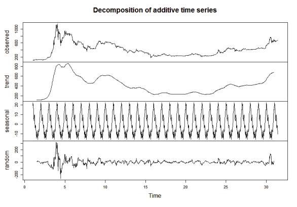
KDD [26] focuses on the prediction task's business setting. The data set utilized by Bitcoin varies from August
19, 2013, to July 19, 2016. Figure 1 gives a time series plot of this. Data from before August 2013 have been
omitted since it no longer depicts the network correctly. Besides CoinDesk's Open, High, Low, Close (OHLC)
statistics, the Blockchain's difficulty and hash rate is taken away. The data have also been standardized for a
mean of 0 and a standard deviation of 1. Standardization was selected over standardization because it best
matches the activation functions of the deep learning models.
Volume XIV, Issue VII, JULY 2021 Page No: 24JAC : A Journal Of Composition Theory ISSN : 0731-6755
Figure 1: Decomposition of the Bitcoin Time Series Data
Evaluation of Feature Engineering and Feature
Feature engineering is the technique of identifying functional patterns from data to facilitate learning their
predictions for machine models. One of the essential elements of data mining may be regarded to obtain good
results in predictive tasks[27],[28]. Several reports have incorporated the Simple Moving Average (SMA)
indicators for machine learning tasks in recent years [29], [30]. A suitable technical indicator example is an
SMA that records the average price over the preceding x days and is also provided.
Boruta (a wrapper constructed around the random method for forest classification) was used to choose
which characteristics to include. This is an ensemble approach in which the voting of many classifications is
carried out. The method is based on a notion similar to that of the random forest classification. It introduces
randomness to the model, gathers data from the random sample collection to evaluate the characteristics, and
offers a clear overview of the critical qualities [31]. All characteristics were judged necessary for the random
forest model, with five days and ten days (by SMA) among the averages evaluated the highest relevance. One
of the essential variables was the de-noised closing price.
III. IMPLEMENTATION
a. RNN
The first argument was the time duration window. As shown by literature support [34], these networks can
struggle with gradient-based optimization to learn long-term dependencies. For the closing price series, an
autocorrelation function (ACF) was used to analyze the connection between the current closing prices and
previous and future closing prices. Although this is no assurance of this predictive power, it was a better
option than a random one. In many cases, the closing price is associated with a delay of up to 20 days, with
individual occurrences of 34, 45 and 47 days. The grid search for the time frame was thus tested from 2 to 20,
34, 45 and 47. More substantial intervals of up to 100 days have also been explored using increments of five
to guarantee a thorough search. The most efficient time frame was 24.
The accuracy of neural network models is a marginal increase over the chances of a binary classification job,
i.e., 50 percent. The RNN has not been used for 50 days while utilizing a temporal length. In contrast, with 100
days generating optimum results, the LSTM performed better in 50 to 100 days.
Table 1: Performance Comparison
Mode
l Epochs CPU GPU
RNN 50 56.71s 33.15s
LSTM 50 59.71s 38.85s
RNN 500 462.31s 258.1s
LSTM 500 1505s 888.34s
RNN 1000 918.03s 613.21s
Volume XIV, Issue VII, JULY 2021 Page No: 25JAC : A Journal Of Composition Theory ISSN : 0731-6755
3001.69 1746.87
LSTM 1000 s s
Table II analyses several models to evaluate the training of the models. The CPU was a 2.6GHz Intel Core. The
GPU utilized was a 940M 2GB NVIDIA GeForce. Both were installed on an SSD on Ubuntu 14.04 LTS. For
comparison, both RNN and LSTM were selected for the identical batch size and period of 50. The GPU
outpaced the CPU significantly. The GPU learned 67.7 percent quicker than the CPU in terms of overall
training time for both networks. The RNN trained on the GPU 58.8% quicker, while the LSTM trained on the
GPU 70.7% faster. The CPU spreads the process over seven threads from monitoring performance in Glances.
The GPU contains 384 CUDA cores that make it more parallel. These models were relatively modest in terms
of two-layer data. For deeper models with more layers or substantial data sets, the advantages of GPU
implementation are higher.
The LSTM takes longer than the RNN with the same network parameters to train due to a higher number of
activation functions and an increase in LSTM equations. This raises the utility of employing an LSTM versus
an RNN due to the additional calculation. Small margins may make all the difference in financial market
predictions. The usage of an LSTM is therefore justified. In other domains, the modest improvement in the
performance of the calculation is not justifiable.
Besides the time window, several hyperparameters also need to be tuned: Learning rate is the parameter that
directs the stochastic descent (SGD), that is to say, how the network learns. Similarly, dynamic updates the
learning rate to prevent the model from slipping into an (error) local minimum and trying to move to a global
bug function minimum [35]. The RMSprop optimizer has been used to enhance SGD, as it maintains a running
average of the recent gradients and is more potent against information loss[36]. According to Heaton[37], the
great majority of nonlinear functions may be approximated by a hidden layer. Two hidden layers were also
investigated and selected since the validation error was more minor. Heaton also suggests the number of
hidden nodes between input and output. Less than 20 nodes per layer led to poor performance in this
scenario.
Good performance was tested for 50 and 100 nodes. But too many nodes might raise the likelihood of
overfitting and considerably increase the time required to train the network. As 20 nodes performed well
enough, the final model was picked. A nonlinear step-by-step equation, which transmits signals across layers,
is also needed. Tanh, ReLu and Sigmoid were the alternatives considered. Tanh did the best, although the
differences were not considered. The final selection criteria are batch size and the number of training periods.
Batch size has minimal influence on accuracy but significantly affects training time in this situation when
utilizing smaller batches.
The number of periods examined ranged from 10 to 10,000, although overfitting can result in too many
training stages. As stated above, dropouts have been incorporated to decrease the danger of overfitting.
Optimal 0.1 to 1 dropout was searched for both layers with 0. 5 dropouts for both layers of the optimum
solution. A Keras callback mechanism was also utilized to terminate training the model if its validation data
performance did not improve after five periods to prevent overfitting. In general, the RNN converged with an
early halt between 20 and 40 epochs.
B. LSTM The LSTM is significantly better at learning long-term dependence in terms of time. This meant that
choosing a lengthy window was less damaging to the LSTM. This technique followed a procedure similar to
the RNN, where the autocorrelation lag was utilized as a guide. The LSTM did not work well in lower window
sizes. Its most effective length was 100 days, and two buried layers of LSTM were selected. Two layers are
Volume XIV, Issue VII, JULY 2021 Page No: 26JAC : A Journal Of Composition Theory ISSN : 0731-6755
adequate to identify nonlinear connections between the data for a time series. Twenty hidden nodes have
also been selected for the RNN model for both layers. The Hyper as Library2 was used to optimize the
network settings in Bayesia. The optimizer looked for the best model regarding how much discontinuation
per layer and what optimizer to apply. RMSprop did the best for this assignment again. Activation functions
have not altered in the LSTM model since the LSTM has a specific sequence of tanning and sigmoid activation
functions for the distinct cell doors.
LSTM models converged with an early halt between 50 and 100 epochs. Similar to the RNN, batch size has a
more significant influence than accuracy on runtime. This might be because the dataset is relatively tiny.
C. Comparison of Models
The ratios of true/false and positive/negative classifications are derived using a confusion matrix. Accuracy
can be defined as the total number of predictions properly categorized (price up, down, and no change). The
sensitivity, specificity and accuracy of measurements are also examined to fight imbalance of classes (bitcoin
price predominately increases). Sensitivity shows how well a model is a positive detection. The specificity
shows how well the model is to avoid false alarms. Finally, precision shows how many forecasts that were
positively categorized were relevant. Root Mean Square Error (RMSE) is utilized for the precise regression
assessment and comparison. An 80/20 holdout validation technique is used to evaluate models.
We have constructed (and optimized) an ARIMA model to allow a comparison of deep learning approaches
with more traditional methods since they were widely utilized in pricing prevision issues (e.g. [38], [39]). The
ARIMA prognosis was developed by dividing the data into five periods and then forecasting the future for 30
days. Before fitting with multiple ARIMA models, the data were differentiated. Auto. Arima from the R
forecast package identified the best fit.
CONCLUSION
Deep learning models such as RNN and LSTM successfully predict Bitcoin with LSTM more capable of
recognizing longer-term relationships. However, such a high variance job makes transpiring this into
outstanding validation findings hard. This remains a challenging process. There's a thin line between
overfitting a model and inhibiting proper learning. Dropout is helpful to help improve this. Despite utilizing
Bayesian optimization to optimize dropout selection, it could not ensure good validation results. Despite
sensitivity, specificity and accuracy measures showing high performance, ARIMA's actual error-based
prediction performance was considerably more flawed than the neural network models. The LSTM
outperforms RNN somewhat, but not much.
LSTM, however, takes much longer to train. The performance benefits of parallelizing machine learning
algorithms on a GPU are evident with a 70.7 percent speed boost for training the LSTM model. Looking at the
problem from a purely perspective categorization, more excellent outcomes can be achieved. The research
drawback is that the model was not deployed in a practical or real-time context to forecast the future instead
of learning what has already happened. Also, the capacity to anticipate utilizing streaming data could enhance
the model. Sliding window validation is not implemented here, although it can be studied as future work. One
difficulty that will occur is that noise naturally hides the data. The difficulty and hash rate variables might be
evaluated for trimming, depending on an examination of the model's weights. Deep learning models require
much data to train successfully. If data granularity were adjusted to every minute, this would give 512,640
data points each year. Such data is not accessible for the past but is being collected daily from CoinDesk for
future use. Finally, algorithm parallelization isn't confined to GPU devices. Field Programmable Gate Arrays
(FPGA) are an exciting alternative to GPU devices, and machine learning models have been proven to perform
better on FPGA than on GPU[40].
Volume XIV, Issue VII, JULY 2021 Page No: 27JAC : A Journal Of Composition Theory ISSN : 0731-6755
REFERENCES
[1] S. Nakamoto, "Bitcoin: A peer-to-peer electronic cash system," 2008.
[2] M. Briere,` K. Oosterlinck, and A. Szafarz, "Virtual currency, tangible return: Portfolio diversification
with bitcoins," Tangible Return: Portfolio Diversification with Bitcoins (September 12, 2013), 2013.
[3] I. Kaastra and M. Boyd, "Designing a neural network for forecasting financial and economic time
series," Neurocomputing, vol. 10, no. 3, pp. 215–236, 1996.
[4] H. White, "Economic prediction using neural networks: The case of IBM daily stock returns," in
Neural Networks, 1988., IEEE International Conference on. IEEE, 1988, pp. 451–458.
[5] C. Chatfield and M. Yar, "Holt-winters forecasting: some practical issues," The Statistician, pp. 129–
140, 1988.
[6] B. Scott, "Bitcoin academic paper database," suitpossum blog, 2016.
[7] M. D. Rechenthin, "Machine-learning classification techniques for the analysis and prediction of high-
frequency stock direction," 2014.
[8] D. Shah and K. Zhang, "Bayesian regression and bitcoin," in Communication, Control, and Computing
(Allerton), 2014 52nd Annual Allerton Conference on. IEEE, 2014, pp. 409–414.
[9] G. H. Chen, S. Nikolov, and D. Shah, "A latent source model for non-parametric time series
classification," in Advances in Neural Information Processing Systems, 2013, pp. 1088–1096.
[10] I. Georgoula, D. Pournarakis, C. Bilanakos, D. N. Sotiropoulos, and G. M. Giaglis, "Using time-series and
sentiment analysis to detect the determinants of bitcoin prices," Available at SSRN 2607167, 2015.
[11] M. Matta, I. Lunesu, and M. Marchesi, "Bitcoin spread prediction using social and web search media,"
Proceedings of DeCAT, 2015.
[12] ——, "The predictor impact of web search media on bitcoin trading volumes."
[13] B. Gu, P. Konana, A. Liu, B. Rajagopalan, and J. Ghosh, "Identifying information in stock message
boards and its implications for stock market efficiency," in Workshop on Information Systems and Economics,
Los Angeles, CA, 2006.
[14] A. Greaves and B. Au, "Using the bitcoin transaction graph to predict the price of bitcoin," 2015.
[15] I. Madan, S. Saluja, and A. Zhao, "Automated bitcoin trading via machine learning algorithms," 2015.
[16] R. Delfin Vidal, "The fractal nature of bitcoin: Evidence from wavelet power spectra," The Fractal
Nature of Bitcoin: Evidence from Wavelet Power Spectra (December 4, 2014), 2014.
[17] L. Kristoufek, "What are the main drivers of the bitcoin price? evidence from wavelet coherence
analysis," PloS one, vol. 10, no. 4, p. e0123923, 2015.
[18] Y. Yoon and G. Swales, "Predicting stock price performance: A neural network approach," in System
Sciences, 1991. Proceedings of the Twenty-Fourth Annual Hawaii International Conference on, vol. 4. IEEE,
1991, pp. 156–162.
Volume XIV, Issue VII, JULY 2021 Page No: 28JAC : A Journal Of Composition Theory ISSN : 0731-6755
[19] T. Koskela, M. Lehtokangas, J. Saarinen, and K. Kaski, "Time series prediction with a multilayer
perceptron, fir and elman neural networks," in Proceedings of the World Congress on Neural Networks.
Citeseer, 1996, pp. 491–496.
[20] C. L. Giles, S. Lawrence, and A. C. Tsoi, "Noisy time series prediction using recurrent neural networks
and grammatical inference," Machine learning, vol. 44, no. 1-2, pp. 161–183, 2001.
[21] A. M. Rather, A. Agarwal, and V. Sastry, "Recurrent neural network and a hybrid model for prediction
of stock returns," Expert Systems with Applications, vol. 42, no. 6, pp. 3234–3241, 2015.
[22] F. A. Gers, D. Eck, and J. Schmidhuber, "Applying lstm to time series predictable through time-window
approaches," pp. 669–676, 2001.
[23] D. Steinkraus, P. Y. Simard, and I. Buck, "Using gpus for machine learning algorithms," in Proceedings
of the Eighth International Conference on Document Analysis and Recognition. IEEE Computer Society, 2005,
pp. 1115–1119.
[24] B. Catanzaro, N. Sundaram, and K. Keutzer, "Fast support vector machine training and classification
on graphics processors," in Proceedings of the 25th international conference on Machine learning. ACM, 2008,
pp. 104–111.
[25] D. C. Ciresan, U. Meier, L. M. Gambardella, and J. Schmidhuber, "Deep, big, simple neural nets for
handwritten digit recognition," Neural computation, vol. 22, no. 12, pp. 3207–3220, 2010.
[26] U. Fayyad, G. Piatetsky-Shapiro, and P. Smyth, "The KDD process for extracting useful knowledge
from volumes of data," Communications of the ACM, vol. 39, no. 11, pp. 27–34, 1996.
[27] T. Dettmers, "Deep learning in a nutshell: Core concepts," NVIDIA Dev blogs, 2015.
[28] D. K. Wind, "Concepts in predictive machine learning," in Maters Thesis, 2014.
[29] Y. Wang, "Stock price direction prediction by directly using prices data: an empirical study on the
kospi and hsi," International Journal of Business Intelligence and Data Mining, vol. 9, no. 2, pp. 145–160, 2014.
[30] S. Lauren and S. D. Harlili, "Stock trend prediction using simple moving average supported by news
classification," in Advanced Informatics: Concept, Theory and Application (ICAICTA), 2014 International
Conference of. IEEE, 2014, pp. 135–139.
[31] M. B. Kursa, W. R. Rudnicki et al., "Feature selection with the boruta package," 2010.
[32] F. Chollet, "Keras," https://github.com/fchollet/keras, 2015.
[33] J. Snoek, H. Larochelle, and R. P. Adams, "Practical bayesian optimization of machine learning
algorithms," in Advances in neural information processing systems, 2012, pp. 2951–2959.
[34] Y. Bengio, "Learning deep architectures for ai," Foundations and Trends R in Machine Learning, vol. 2,
no. 1, pp. 1–127, 2009.
[35] L. Yu, S. Wang, and K. K. Lai, "A novel nonlinear ensemble forecasting model are incorporating glar
and ann for foreign exchange rates," Computers And Operations Research, vol. 32, no. 10, pp. 2523–2541,
2005.
Volume XIV, Issue VII, JULY 2021 Page No: 29JAC : A Journal Of Composition Theory ISSN : 0731-6755
[36] G. Hinton, N. Srivastava, and K. Swersky, "Lecture 6a overview of mini-batch gradient descent,"
Coursera Lecture slides https://class. Coursera. org/neural nets-2012-001/lecture,[Online.
[37] J. Heaton, "Introduction to the neural network for java, Heaton research," Inc. St. Louis, 2005.
[38] J. Contreras, R. Espinola, F. J. Nogales, and A. J. Conejo, “Arima models to predict next-day electricity
prices,” IEEE transactions on power systems, vol. 18, no. 3, pp. 1014–1020, 2003.
[39] P.-F. Pai and C.-S. Lin, "A hybrid Arima and support vector machines model in stock price
forecasting," Omega, vol. 33, no. 6, pp. 497–505, 2005.
[40] M. Papadonikolakis, C.-S. Bouganis, and G. Constantinides, "Perform-ance comparison of GPU and
FPGA architectures for the SVM training problem," Field-Programmable Technology, 2009. FPT 2009.
International Conference on. IEEE, 2009, pp. 388–391.
Volume XIV, Issue VII, JULY 2021 Page No: 30You can also read