A Hidden Markov Model-Based Acoustic Cicada Detector for Crowdsourced Smartphone Biodiversity Monitoring
←
→
Page content transcription
If your browser does not render page correctly, please read the page content below
A Hidden Markov Model-Based Acoustic Cicada Detector for
                    Crowdsourced Smartphone Biodiversity Monitoring

                        Davide Zilli, Oliver Parson, Geoff V Merrett, Alex Rogers
              Electronics and Computer Science, University of Southampton, Southampton, UK
                           {dz2v07,op106,gvm,acr}@ecs.soton.ac.uk

                          Abstract
     Automated acoustic recognition of species aims
     to provide a cost-effective method for biodiversity
     monitoring. This is particularly appealing for de-
     tecting endangered animals with a distinctive call,
     such as the New Forest cicada. To this end, we pur-
     sue a crowdsourcing approach, whereby the mil-
     lions of visitors to the New Forest will help to mon-
     itor the presence of this cicada by means of a smart-
     phone app that can detect its mating call. However,           Figure 1: Cicadetta montana. Photograph by Jaroslav Maly,
     current systems for acoustic insect classification are        reproduced with permission.
     aimed at batch processing and not suited to a real-
     time approach as required by this system, because
                                                                   due to climate change or land-use change, is an important
     they are too computationally expensive and not ro-
                                                                   question for UK biodiversity research.
     bust to environmental noise. To address this short-
                                                                      Today, traditional approaches to searching for rare species
     coming we propose a novel insect detection algo-
                                                                   typically call for trained ecologists to perform detailed man-
     rithm based on a hidden Markov model to which
                                                                   ual surveys. However, the obvious costs of such work have
     we feed as a single feature vector the ratio of two
                                                                   led to significant recent research into automated approaches
     key frequencies extracted through the Goertzel al-
                                                                   whereby animals and plants can be classified remotely with-
     gorithm. Our results show that this novel approach,
                                                                   out requiring that trained experts be in the field. In the
     compared to the state of the art for batch insect clas-
                                                                   case of insects, this is most often performed by deploy-
     sification, is much more robust to noise while also
                                                                   ing fixed sensors with sensitive microphones that record the
     reducing the computational cost.
                                                                   sounds that the insects emit [MacLeod, 2007]. These record-
                                                                   ings are then analysed later to automatically identify the in-
                                                                   sects whose calls were heard. The algorithms to do so typ-
1   Introduction                                                   ically range from those that operate solely in the time do-
Biodiversity is a key measure of the health of an ecosystem,       main, such as time domain signal coding [Chesmore, 2004;
and as land-use and climate change impact on the natural en-       Chesmore and Ohya, 2004], to those inspired by the litera-
vironment, many countries are increasingly seeing the need to      ture of human speech recognition. The latter typically use
monitor and protect it. For example, the UK has formalised         a hidden Markov model (HMM) for classification [Leqing
this within the UK Biodiversity Action Plan (UK BAP) and           and Zhen, 2010], and perform a number of pre-processing
has established a priority species list to focus work on a small   stages, often taken directly from the human speech recogni-
number of critically important species [Joint Nature Conser-       tion literature, to extract features from the raw recording. For
vation Committee, 2010]. One of these, of particular interest      example, [Chaves et al., 2012] present a state-of-the-art ap-
in this paper, is the New Forest cicada (cicadetta montana s.      proach that pre-processes the recorded sound to remove un-
str., see Figure 1); the only native cicada known to the UK,       sounded periods where no insect call is detected, that maps
which was first identified in the New Forest, a national park      the raw frequencies to the mel scale, which better represents
on the south coast of England, in 1812. Despite being well         human hearing; then it converts it back into a pseudo-time do-
studied at a number of sites in the 1960s, there has been no       main, called the cepstrum, by calculating a number of mel fre-
confirmed observation of the New Forest cicada in the last 20      quency cepstral coefficients (MFCC), that are used as features
years [Pinchen and Ward, 2002]. Understanding whether this         for the HMM classification with just one state per species.
is simply due to the migration of the cicada to as yet undis-         The use of automatic acoustic recognition is particularly
covered sites, or whether the cicada is now extinct in the UK      appealing in the case of the New Forest cicada, since this in-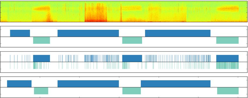
sect has a particularly loud high-pitched mating song which,        tection and recognition of insects (and specifically, the New
while being close to the upper frequency limit of a normal          Forest cicada) on computationally constrained smartphones.
adult hearing range, can easily be detected by conventional         Rather than calculating a number of mel frequency cepstral
microphones. However, the use of fixed sensors to collect           coefficients, as above, we use the Goertzel algorithm — an
these recordings for later analysis is less compelling. The         efficient method for approximating individual terms of a dis-
New Forest covers 600 km2 , and, to exhaustively survey it for      crete Fourier transform (DFT) [Goertzel, 1958] — to calcu-
potential cicada breeding sites, would require tens of thou-        late the magnitude of two specific frequency bands; one cen-
sands of sensors. Therefore, in our work, we are pursuing           tred at 14 kHz, corresponding the central frequency of both
a different approach, and are seeking to exploit the 13 mil-        the insects’ calls, and one centred at 8 kHz, which is far from
lion day visits to the New Forest that occur each year by the       both general background noise and the insects’ call. We use
general public to crowdsource the search for the New Forest         the ratio of these magnitudes as a single feature, which iden-
cicada. In particular, in this paper, we describe a HMM-based       tifies the song of either the bush cricket or the New Forest ci-
detection algorithm that runs within a smartphone app, to be        cada. Then, we use a four-state hidden Markov model that ex-
used by these visitors, that can automatically detect the mat-      plicitly represents both the idle, un-sounded period between
ing call of the male cicada, identify it as such to the user in     insect calls, and also the short pauses between the chirps
real-time, and prompt the user to make a recording that can         of the bush cricket’s song. Hence, rather than attempting
be uploaded for further analysis once the smartphone has an         to recover the time domain information lost while removing
acceptable Internet connection. A similar approach to crowd-        un-sounded periods through heuristic methods, we explicitly
sourcing for sustainability problems using mobile phones was        capture this in the HMM, as this approach can be readily ex-
employed by Quinn et al. [2011], however it has not yet been        tended to cover insect calls of more complexity, all within the
applied to crowdsourcing biodiversity using acoustics.              same principled framework. We then use the Viterbi algo-
   The requirements of the automatic detection algorithm that       rithm to identify the most likely sequence of insect calls at
will run on these smartphones are somewhat different to those       any point in time, as in Sun et al. [2009].
that have been previously proposed for post recording analy-            We evaluate our approach using recordings made by the au-
sis of insect calls. Firstly, we must be aware of the limited       thors with an Apple iPhone 4S of both the New Forest cicada
computational resources available on some lower-end mobile          (recorded in Slovenia where the same species is still abun-
devices. The algorithms described above are typically de-           dant) and the dark bush cricket (recorded in the New For-
signed to run on high-end servers, and thus, are relatively         est). Unlike standard library recordings, our trial dataset rep-
unconstrained by both memory and processor speed. Sec-              resents the quality of crowdsourced data that we are likely
ondly, we note that the algorithms above are designed to run        to encounter, exhibiting significant noise (including, among
in batch-mode on existing recordings, whereas in our appli-         others, handling noise, background road traffic, human voice
cation, we require that the algorithms provide real-time feed-      and noise generated by the wind), and insect calls of varying
back to the user as to the identification of the insect being       amplitude depending on the proximity of the recording device
heard; firstly, so that if it is not a cicada we do not force the   to the specimen.
user to upload unnecessary recordings1 , and conversely, if a           We show how our approach is capable of identifying the ci-
cicada is detected, so that we can prompt the user to collect       cada call in normal environmental noise more accurately than
the best quality recording possible and keep them engaged in        the state-of-the-art batch classification algorithms described
the search. Finally, the pre-processing approaches described        earlier. In particular, we achieve an F1 score of 0.955 for the
above may actually impair detection in certain cases. In par-       detection of the cicada on a large data set of over 30 calls,
ticular, while often insects can easily be classified by differ-    recorded with a smartphone, while the method proposed by
ences in the frequencies of their song, we demonstrate that         Chaves et al. [2012] only scores F1 = 0.126 due to the con-
these methods fail to distinguish between the song of the           fusion with the cricket’s calls. Our efficient feature extraction
New Forest cicada (which sings continuously at 14 kHz),             procedure is robust to noise and decreases the computational
and that of the dark bush cricket, common in the New For-           complexity of the detection process, providing the capability
est (that chirps intermittently at 14 kHz). This is because         for real time classification.
the conversion of the raw frequency domain data into mel                The remainder of this paper is organised as follows. In
frequency cepstral coefficients fails to generate any distin-       Section 2, we describe our proposed approach, highlighting
guishing features in the frequency-domain (since the mel fre-       the different techniques used. In Section 3 we analyse its per-
quency conversion has poor resolution at high frequencies,          formance in comparison to a state-of-the-art model for batch
being intended for the much lower frequencies which con-            classification, providing the relevant accuracy metrics. We
stitute typical human speech), while the automatic removal          conclude in Section 4 along with an overview of future work.
of un-sounded periods from the recording also removes the
time-domain features which would have differentiated them.          2   Real-Time Insect Detection Using Hidden
   Thus, to address these shortcomings, in this paper we
present an algorithm specifically intended for real-time de-
                                                                        Markov Models
                                                                    We now give a description of our proposed approach for real-
   1
    A 60s mono recording at 44,100 samples per second, is about     time insect detection. We first describe a method by which
5MB; a significant file to upload in areas with poor mobile phone   we efficiently extract individual terms of a DFT from the raw
reception where connection rates may be down to 100kbps or less.    audio recordings using the Goertzel algorithm. We then de-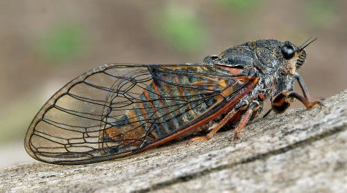
z1         z2           z3                         zT

                                                                          x1         x2           x3                         xT

                                                                    Figure 3: A hidden Markov model. Unshaded square nodes
Figure 2: Spectrogram and waveform of a New Forest cicada           represent observed discrete variables, while shaded circular
call (recording by Jim Grant, 1971 and courtesy of the British      nodes represent hidden continuous variables.
Library, wildlife sounds collection).

                                                                       In terms of computational complexity, this approach shows
scribe how two of these terms can be combined to produce a          a considerable benefit compared to the single-bin DFT. An
feature that is robust to noise. Last, we show how this feature     efficient algorithm to compute the latter, the fast Fourier
is used to classify periods of a recording to a particular insect   transform (FFT), has a complexity of O(N logN ), while the
using a four-state HMM.                                             Goertzel algorithm is only computed in order O(N ), where
2.1   Feature Extraction Using Goertzel Algorithm                   N is the number of samples per window. Moreover, the sam-
                                                                    ple update described in equation 5 can be processed in real-
For the purposes of our system, it was observed that the call       time, eliminating the need for an independent background
of the New Forest cicada displays a strong frequency compo-         thread on the smartphone app.
nent centred around 14 kHz (see Figure 2). This frequency is
sufficiently distant from any common background noise, such         2.2    Feature Combination Using Filter Ratio
as wind noise, road traffic or people speaking, to be a reliable    The magnitude of the frequency component at 14 kHz is a
identifier of the presence of the cicada. An efficient approx-      good indicator of the presence of a New Forest cicada, ro-
imation of the magnitude of this given frequency can be cal-        bust against generic background noise. However, it may be
culated using the Goertzel algorithm, a method that evaluates       sensitive to white noise that covers the entire frequency spec-
individual terms of a DFT, implemented as a second order            trum, such as handling noise. Therefore, in order to reduce
infinite impulse response (IRR) filter.                             this sensitivity, we divide the magnitude of this feature by the
   An efficient implementation of the Goertzel algorithm re-        magnitude observed around 8 kHz, also computed with the
quires two steps. The first step produces a coefficient that can    Goertzel algorithm described above. This band is outside the
be pre-computed and cached to reduce CPU cycles:                    range of both the cicada call and environmental noise. Hence,

                                    2πf
                                                                   this ratio will be high in the presence of a cicada and tend to
                        c = 2 cos                             (1)   zero when either no sound is detected in the cicada range or
                                     fs
                                                                    if sound is present across both bands. The ratio of the se-
where f is the central frequency in question and fs the sam-        quences of these two terms mf,1 , . . . , mf,T , computed over
pling rate of the recording.                                        time T , results in the feature vector x = x1 , . . . , xT such
   The second step consists of iteratively updating the values      that:
                                                                                                     m14
of a temporary sequence y with any incoming sample s such                                       x=                               (6)
that:                                                                                                m8
           yn = hamming(s) + (c · yn−1 ) − yn−2            (2)         Once the ratio between the 14 kHz and 8 kHz frequencies
                                                                    has been calculated, this can be used as a single feature vec-
where the samples are passed through a Hamming filter, given
                                                                    tor, x, for our classification model. In order to obtain real-
by:
                                               2πs
                                                                   time computationally efficient insect identification, we adopt
         hamming(s) = 0.54 − 0.46 cos                      (3)      a HMM based approach to classification.
                                             N −1
and the length of the sequence of samples N determines the          2.3    Classification Using Four-State HMM
bandwidth B of the Goertzel filter, such that:                      A HMM consists of a Markov chain of discrete latent vari-
                                  fs                                ables and a sequence of continuous observed variables, each
                           B=4                             (4)      of which is dependent upon one discrete variable’s state
                                  N                                 [Blasiak and Rangwala, 2011]. Figure 3 shows the graphical
   A sequence length N yields larger bandwidth, at the cost of      structure of a HMM, where the discrete, hidden variables (the
a noisier output. In practice, we use multiples of 64 samples       singing states) are represented by the sequence z1 , . . . , zT ,
to match a typical smartphone’s buffer size. For example, a         and the continuous, observed variables (the song feature) are
block size N = 128 samples gives a bandwidth of just under          represented by the sequence x1 , . . . , xT . The value of each
1.4 kHz. The magnitude m of the frequency band centred at           discrete variable zt corresponds to one of K states, while each
f and with bandwidth B is then given by:                            continuous variable can take on the value of any real number.
                   q                                                   The behaviour of a hidden Markov model is completely de-
                       2 + y2
            mf = yN           N −1 − c · yN · yN −1        (5)      fined by the following three parameters. First, the probability
0.12 Log-normal emission B
probabilities
Probability Density Function
0.10 Empirical data for
cicada call BC BSP
0.08
0.06
0.04 I C
0.02
0.00
0 10 20 30 40 50 Figure 5: Four-state finite state machine. BC represents the
Feature Value (xt )
bush cricket’s chirp, BSP represents the short pause between
Figure 4: Log-normal distribution of the extracted feature for chirps, I represents the idle state and C represents the ci-
the cicada call cada’s song.
of each state of the hidden variable at t = 1 is represented by C B
the vector π such that:
πk = p(z1 = k) (7)
Figure 6: Two-state finite state machine. C represents the
Second, the transition probabilities from state i at t − 1 to cicada’s song and B represents the cricket’s chirp.
state j at t are represented by the matrix A such that:
Ai,j = p(zt = j|zt−1 = i) (8) cricket is chirping (BC ) and a short pause in between the
Third, the emission probabilities that describe the observed dark bush cricket’s chirps (BSP ). The model parameters µ
feature, x, given parameters φ, follow a log-normal distribu- and σ 2 are learned empirically for each state k using:
tion such that: PT PT
t=1 ln(xt ) 2 (ln(xt ) − µ)2
xt |zt , φ ∼ ln N (µzt , σz2t ) (9) µk = , σk = t=1 (11)
T T
where φ = {µ, σ 2 }, and µzt and σz2t are the mean and vari- The transition matrices describing the dynamics of a
ance of the Gaussian distribution for state zt . Figure 4 shows Markovian process can be represented graphically using fi-
a histogram of data generated by a cicada’s song, along with nite state machines. Figure 5 shows the four states described
our log-normal distribution fitted to the data. Despite the dis- above and all possible transitions, where those with non-zero
tribution’s long tail, it still has poor support for data of un- probability are represented by arrows connecting two states.
usually high magnitude, as are often generated by handling Our model explicitly represents the silence between the dark
noise. In order to prevent the model from strongly favouring bush cricket song, which is essential information for distin-
a certain state when a data point is in the extreme of the log- guishing between the two insects’ songs. This is in contrast
normal distribution, we add a uniform term over all emission to the model used by Chaves et al. [2012], in which each in-
probabilities, with small probability, to capture cases where sect is represented by a single state, as shown by Figure 6.
our data are likely to be poorly represented. Having presented our model, we now go on to compare its
Equations 7, 8 and 9 can then be used to calculate the joint performance to the more complex system for batch process-
likelihood of a hidden Markov model: ing proposed by Chaves et al. [2012]. This system mimics a
T T
standard speech recognition model based on HMMs.
Y Y
p(x, z|θ) = p(z1 |π) p(zt |zt−1 , A) p(xt |zt , φ) (10)
t=2 t=1 3 Empirical Evaluation Using Smartphone
where the model parameters are defined by θ = {π, A, φ}. Recordings
We use the Viterbi algorithm to infer the most likely se- We compare our approach, as described in Section 2, to the
quence of hidden states given the features described. Despite state-of-the-art approach used by [Chaves et al., 2012]. In the
the fact that the number of possible paths grows exponentially latter, the signal is firstly stripped of un-sounded areas and
with the length of the chain, this algorithm efficiently finds segmented to extract individual calls. It is then pre-processed
the most probable sequence by maximising Equation 10, with by removing the DC offset, dividing it into frames, empha-
a cost that grows only linearly with the length of the chain. sising high frequencies, and passing it through a windowing
function. The windows are then run through a FFT and con-
2.4 Finite State Model of Insect Call verted into the mel frequency scale, from which the mel fre-
We propose a four-state HMM for cicada detection, in which quency cepstral coefficients are generated. These are used as
the states consist of: an idle state in which no insect is singing individual features for a simple HMM. For the recording in
(I), a cicada singing state (C), a state where the dark bush analysis, this consists of two states, one for the cicada and one20
Freq (kHz)
15
(a) 10
5
0
Ground Truth
B
(b) I
C
Chaves 2012
B
(c) I
C
B
Our Model
(d) I
C
0 50 100 150 200 250 300
Time(s)
Figure 7: The proposed model, run on a recording with several dark bush cricket’s calls and three cicada songs. I, C and B
represent the idle, cicada and cricket states respectively, as in Figure 5. B encompasses both the cricket’s chirping (BC ) and
short pause (BSP ) states.
for the bush cricket, with a feature vector of 24 cepstral co- reintroduced in the output for the sake of comparison. On the
efficients, each assumed to be normally distributed. No state plot they are marked as idle, although the model itself does
for silence is considered, as this has been removed during the not account for an idle state. Since the comparison is focused
pre-processing stage. on the discernment of the two insects rather than the detec-
tion of sounded and un-sounded areas we manually label the
To evaluate the accuracy of our approach, we collected
sounded and un-sounded areas. Finally, Figure 7d shows the
recordings of the New Forest cicada from a known habitat
output of the model proposed in this paper. The two states
in Slovenia and the dark bush cricket from the New Forest
used to identify the dark bush cricket’s call are merged into
using an Apple iPhone 4S. In contrast to existing recording
one, again as represented in Figure 5. It is immediately appar-
libraries, this data set represents the quality of crowdsourced
ent how closely our proposed approach matches the ground
data that we are likely to encounter, exhibiting significant
truth in comparison to Chaves et al. [2012].
noise (including, among others, handling noise, background
road traffic, human voice and noise generated by the wind), It emerges clearly that removing silence between calls also
and insect calls of varying amplitude depending on the prox- removes the time domain features crucial at discerning these
imity of the recording device to the specimen. two insects. The output of the HMM in Figure 7c, displays
confusion between the chirping call and the prolonged call
Figure 7 shows a comparison of the two approaches us-
and is unable to identify them correctly. The visual intuition
ing a concatenation of three cicada calls and several instances
is confirmed by the accuracy measures described below and
of the dark bush cricket call intertwined. Figure 7a shows
reported in Table 1. On the contrary, our proposed model is
a spectrogram with the time domain on the x-axis, and the
able to take advantage of the clear time-domain feature and,
frequency domain on the y-axis, with the magnitude of the
despite the emission probabilities of the two sounded and the
frequency bins varying with the colour of the plot. The three
two un-sounded states being identical, the transition proba-
cicada calls can be identified as the prolonged strong compo-
bilities ensure that prolonged periods of silence are classi-
nent in the high frequency band. The chirping calls are visi-
fied as the idle state. To this extent, the backward pass of
ble as thin vertical bars on the top half of the spectrum. Note
the Viterbi algorithm ensures that any mistakes due to a state
that the different recordings, merged together into this data
having the highest local probability are corrected to provide
set, have varying background noise, identifiable particularly
the most likely overall path. Furthermore, this approach can
as high magnitude components at the bottom of the spectrum.
be readily extended to calls of more complexity by further
Figure 7b shows the ground truth, labelled manually, i.e. the
increasing the number of sub-states attributed to each insect.
correct classification of the different insects. The states are
labelled as in Figure 5, where I represents the un-sounded We assess the accuracy by which each approach can cor-
idle state, C represents the cicada’s song and B represents rectly classify the cicada using the standard precision, recall
both the bush cricket’s chirping and short pause states. Figure and F1 score metrics. The precision represents the fraction
7c shows the output of the model from Chaves et al. [2012]. of time slices in which the approach detected the cicada as
For this approach, areas identified as idle have been removed singing when it was in fact singing, while the recall represents
from the feature by the pre-processing stage, but have been the fraction of time slices in which the cicada was singing thatApproach Precision Recall F1 -score
Our approach 1.000 0.914 0.955
Chaves et al. [2012] 0.563 0.071 0.126
Table 1: Accuracy metrics of cicada detection
were correctly detected. Precision and recall are defined as:
tp
precision = (12)
tp + f p
tp
recall = (13)
tp + f n
where tp represents the number of correct cicada song de-
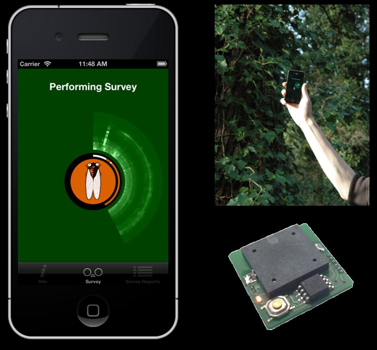
tections, f p represents the number of cicada song detections Figure 8: Prototype app interface showing the real-time feed-
when it was actually not singing, and f n represents the num- back presented to the user during a 60 second survey, indicat-
ber of cicada songs which were not detected. In this work, ing the detection of a cicada song, and the electronic cicada
we are not concerned by the accuracy of the cricket’s detec- that replicates the sound of the cicada, used for user testing.
tion. We also use the F1 score, which represents a weighted
combination of precision and recall, defined as:
precision · recall execution times of both approaches were evaluated on a mid-
F1 = 2 · (14) range modern computer (Intel Core 2 Duo CPU, 2.4 GHz,
precision + recall 8 GB RAM), with the software entirely written in Python.
Table 1 shows the precision, recall and F1 score metrics
both for the approach described in this paper and that used by 4 Conclusions
Chaves et al. 2012 over a much larger data set of over 30 dif-
In this paper we have presented a novel automated insect de-
ferent cicada songs. It is clear that the approach proposed by
tection algorithm that, to the best of our knowledge, is the first
Chaves et al. [2012] fails to distinguish between the cicada’s
targeted at real-time identification of selected species. We
song and the bush cricket’s chirp, resulting in poor precision
have shown that with a careful analysis of the call to be de-
and recall statistics. Conversely, both the precision and recall
tected, key features can be extracted at minimal cost, greatly
metrics for our proposed approach are close to 1, as a result
simplifying the identification process. We compared our ap-
of our model’s ability to use the periods between the bush
proach with a state-of-the-art technique, and identified sce-
cricket’s chirps to differentiate between the two songs. Fur-
narios where such a technique would fail to distinguish two
thermore, the vastly greater precision and recall metrics for
given calls in a smartphone recording.
our proposed approach have resulted in a greater F1 score.
Our results show that the proposed system achieves an ac-
Our approach’s F1 score can be interpreted as a suitable trade
curacy of F1 = 0.955 on a data set of recordings taken with
off between false detections and missed detections.
an Apple iPhone 4S at 44,100 kHz in their original sound-
It is also worth comparing the computational efficiency of
scape, which includes various forms of background noise and
the approach used by Chaves et al. [2012] to the approach
different animal calls, as well as human voice, interfering
described in this paper. In the Chaves et al. [2012] model,
with the signal. Rather than focusing on batch processing
the two most costly operations, namely the sound detection
of large data sets of species, our approach aims at identifying
algorithm and the computation of the cepstral coefficients,
a small number of species in real time.
both require an order O(N logN ) to compute, with N being
With the development of the robust acoustic classifier com-
the number of samples in the recording. In comparison, the
plete, we have integrated the technology into the prototype
entire feature extraction process in our proposed model only
smartphone app shown by Figure 8. We are currently carry-
requires O(N ) operations. This complexity corresponds to
ing out user testing of the app through the use of an electronic
a computation time of 537s for the Chaves et al. [2012] ap-
cicada, a stand-alone circuit board and speaker that replicates
proach, while our approach takes 45s to process the record-
the sound of the New Forest cicada’s song. The project will
ing of length 311s, shown in Figure 7. Since the Chaves et
launch publicly in June 2013, and will constitute the first live
al. [2012] method takes longer to run than the length of the
crowdsourced system to search for an endangered species of
recording, clearly it is not efficient enough to run in real-time.
insect of national importance.
In comparison, our approach processed the whole recording
in one seventh of the recording time, and therefore is suitable
to run in real-time. These values, although dependent on im- Acknowledgements
plementation details, corroborate the hypothesis that the for- This research was supported by an EPSRC Doctoral Training
mer model has a considerably higher computational complex- Centre grant (EP/G03690X/1) and by the ORCHID Project,
ity, as shown in Section 2. This, together with the increased www.orchid.ac.uk (EP/I011587/1). Many thanks to Dr Tomi
robustness to noise shown by the accuracy metrics, allows us Trilar and Prof Matija Gogala for their field guidance in
to conclude that our model is better suited to real-time de- Slovenia and to Dr David Chesmore for his original sugges-
tection than the state of the art for insect classification. The tion and ongoing support.References [Blasiak and Rangwala, 2011] S. Blasiak and H. Rangwala. A hidden markov model variant for sequence classifica- tion. In Proceedings of the Twenty-Second International Joint Conference on Artificial Intelligence, pages 1192– 1197. Barcelona, Catalonia, Spain, 2011. [Chaves et al., 2012] V. A. E. Chaves, C. M. Travieso, A. Ca- macho, and J. B. Alonso. Katydids acoustic classification on verification approach based on MFCC and HMM. Pro- ceedings of the 16th IEEE International Conference on Intelligent Engineering Systems (INES), pages 561–566, 2012. [Chesmore and Ohya, 2004] E. D. Chesmore and E. Ohya. Automated identification of field-recorded songs of four British grasshoppers using bioacoustic signal recogni- tion. Bulletin of Entomological Research, 94(04):319– 330, 2004. [Chesmore, 2004] E. D. Chesmore. Automated bioacoustic identification of species. Anais da Academia Brasileira de Ciências, 76(2):436–440, 2004. [Goertzel, 1958] G. Goertzel. An algorithm for the evalua- tion of finite trigonometric series. The American Mathe- matical Monthly, 65(1):34–35, 1958. [Joint Nature Conservation Committee, 2010] Joint Nature Conservation Committee. UK priority species pages Ci- cadetta montana (New Forest Cicada). Technical report, 2010. [Leqing and Zhen, 2010] Z. Leqing and Z. Zhen. Insect Sound Recognition Based on SBC and HMM. In Inter- national Conference on Intelligent Computation Technol- ogy and Automation (ICICTA), volume 2, pages 544 –548, 2010. [MacLeod, 2007] Norman MacLeod. Automated Taxon Identification in Systematics: Theory, Approaches and Ap- plications. CRC Press, 2007. [Pinchen and Ward, 2002] B. J. Pinchen and L. K. Ward. The history, ecology and conservation of the New Forest Ci- cada. British Wildlife, 13(4):258–266, 2002. [Quinn et al., 2011] J. Quinn, K. Leyton-Brown, and E. Mwebaze. Modeling and monitoring crop disease in developing countries. In Proceedings of the Twenty-Fifth Conference of the Association for the Advancement of Artificial Intelligence. San Francisco, CA, USA, 2011. [Sun et al., 2009] X. Sun, T. Matsuzaki, D. Okanohara, and J. Tsujii. Latent variable perceptron algorithm for struc- tured classification. In Proceedings of the Twenty-First International Joint Conference on Artificial Intelligence, pages 1236–1242. Pasadena, California, USA, 2009.
You can also read