A continuous-time Markov process for mobility in the labor market: the impact of breast cancer diagnosis in the case of French females
←
→
Page content transcription
If your browser does not render page correctly, please read the page content below
A continuous-time Markov process for mobility in the labor
        market: the impact of breast cancer diagnosis in the case of
                            French females*

      Vanessa BASCETTO1,2,3; Jean-Paul MOATTI1,2,3; Alain PARAPONARIS1,2,3; Luis SAGAON TEYSSIER1,2,3,4

1
    INSERM, U912 (SE4S), Marseille, France
2
    Université Aix-Marseille, IRD, UMR-912, Marseille, France
3
    ORS PACA, Observatoire Régional de la Santé Provence Alpes Côte d’Azur Marseille France
4
    GREQAM, CNRS Research Unit 6579, Marseille

                                                       Abstract
This article investigates whether a cancer event might be transformed into a permanent loss in employment
conditions. For this, we re-evaluate the impact of cancer on labor market conditions using comparative transition
matrices between occupational states. We obtain a set of statistics based on estimations using continuous-time
Markov transition processes, and we employ these to study and compare labor market dynamics in two
populations: individuals diagnosed with cancer and their counterparts in the general population matched with
propensity score. The consequences of cancer diagnosis were measured by a significant deviation in the
transition matrix for cancer survivors as compared to a prior matrix standardized based on the general
population. Data were stratified by social class, first to allow for a clear separation with regard to cancer-specific
impacts, and second to take into account other stigmas in the labor market that are inherent to the subpopulations
we examined. We also consider systematic differences in socioeconomic status and the ability to return to work.

Keywords Breast cancer survivors, mobility in the labor market, Markov modeling

* The authors thank the members of the Cancer Study Group (Groupe d’Etude ALD Cancer) : Guy-Robert Auleley (Caisse
nationale du RSI, Paris), Pascal Auquier (Université de la Méditerranée, Marseille), Philippe Bataille (Université Lille 3,
Lille), Nicole Bertin (CNAMTS, Paris), Frédéric Bousquet (HAS, Paris), Anne-Chantal Braud (Institut Paoli-Calmettes,
Marseille), Chantal Cases (IRDES, Paris), Sandrine Cayrou (Toulouse),Claire Compagnon (Paris), Paul Dickes (Université
Nancy 2 - GRAPCO - LABPSYLOR, Nancy), Pascale Grosclaude (Registre du cancer du Tarn, Albi), Anne-Gaëlle Le
Corroller-Soriano (INSERM 912, Marseille), Laëtitia Malavolti (INSERM 912, Marseille), Catherine Mermilliod (DREES,
Paris), Jean-Paul Moatti (Université de la Méditerranée & INSERM 912, Marseille), Nora Moumjid-Ferdjaoui (GRESAC -
Université Lyon 1, Lyon), Marie-Claude Mouquet (DREES, Paris), Lucile Olier (DREES, Paris), Frédérique Rousseau
(Institut Paoli-Calmettes, Marseille), Gérard Salem (InCa, Paris),Christine Scaramozzino (Ligue Nationale contre le Cancer,
Paris), Florence Suzan (Institut de Veille Sanitaire, Saint-Maurice), Vincent Van Bockstael (CCMSA, Paris), Alain Weill
(CNAMTS, Paris). The Cancer Study has been realized with the joining efforts of the Department for Research, Studies,
Assessment and Statistics (DREES) of the French Health Ministry, the Inserm Research Unit 912 (Economic & Social
Sciences, Health Systems & Societies), the three major sickness funds and their medical department (CNAMTS, CCMSA and
Caisse Nationale du RSI) and the Ligue Nationale contre le Cancer. They also thank Sophie Eichenbaum-Voline (INSERM
912, Marseille) for research assistance.
Grant from the program Workplace position and careers of cancer survivors financed by the French National Cancer Institute
(Institut National du Cancer, InCa) and the National Agency for Research (ANR) within the program Vulnerabilities: the
articulation of health and social is greatly acknowledged.
Correspondence should be sent to: luis.sagaon_teyssier@etumel.univmed.fr (Luis SAGAON TEYSSIER)

                                                                                                                         1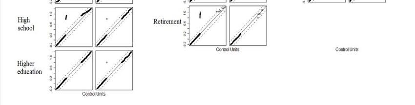
Introduction

The importance of cancer in general public health, as well as in the day-to-day lives of many
among us, is self-evident. During the last 20 years, breast is the most frequent localization of
mortal cancers for females in France. At the same time, the mortality rate of cancer has
declined of almost 1.5 percentage point between 1990 and 2002 (the mortality rate passed
from 34.5% to 33%). Moreover, in the recent years, deaths occur relatively more in late-age
categories. These features reflect the improvement of the diagnosis procedures, the prevention
methods and a better care providing which extend the life expectancies of diagnosed females.
Consequently, an increasing number of cancer survivors return to work after their treatment or
while they are being treated. However, during and after these treatments, patients face
physical and psychological after-effects that likely impact many aspects of their day-to-day
lives, including their professional lives.

Previous studies have shown that a change of job or employer, a shift to part-time work,
unemployment, and early retirement are common among cancer survivors (Short et al., 2005).
Meanwhile, a return to work after treatment is associated with a better quality of life
(Hoffman, 1999; Spelten et al., 2002; Bloom et al., 2004). In addition, the previous research
points to a number of ways in which cancer may affect employment, including physical
limitations (Chirikos et al., 2002; Bradley and Bednarek, 2002), emotional problems
(Greaves-Otte et al., 1991), difficulties with concentration and memory (Schagen et al., 1999)
and changing personal priorities (Maunsell et al., 1999; Hoffman, 2005). Negative
interactions with co-workers (Greaves-Otte et al., 1991; Maunsell et al., 1999) and employers
are also an ongoing concern. A recent paper (Short et al., 2005) concluded that “efforts to
quantify employment problems associated with cancer survival have been hampered by small
sample sizes, lack of longitudinal data, and an inability to account for differences by cancer
site”.

In this paper, we propose statistics based on estimations generated using continuous-time
Markov transition processes. The method for estimating probabilities of transitions’ matrices
closely follows the work of Fougère and Kamionka (1992). Our analysis is also enriched by
two matched databases: individuals diagnosed with cancer and a control group sampled from
the general population. Propensity scores are used for matching. This method makes possible
two new contributions to the literature:

   •   The capacity to account for the role of cancer diagnosis in explaining differences in
       returning to work among the non-employed. One of the main goals of the paper is that
       we take into account transitions not only from employment to non-employment, but
       also among various states.
   •   We use our estimations to simulate the probabilities of staying employed after the
       diagnosis, or leaving employment. At the same time the simulation of the job loss is
       made taken into account two possible exits towards non-employment or towards
       retirement. These simulations give an idea of the consequences that the breast cancer
       diagnosis has in the long-run.

The paper is organized as follows. Section 2, presents the data and the matching strategy used
to link cancer survivors to their counterparts taken from a general survey on employment. The
section 3, is devoted to the presentation of the continuous-time Markov model. The results
about the impact of cancer upon mobility are presented in the section 4 by taking into account
the role of the SES. Finally, we discuss our results in the section 5.

                                                                                              2
2. The data and the propensity score matching process: reduction of the sample bias
between the cancer survivors and the general population
In this paper, we use two databases. The first database was collected by the French Health
Ministry in late 2004 and includes information about the living conditions of adult patients
diagnosed with cancer between September and October 2002. The second database is the
employment survey (ES) conducted by the National Institute of Statistics and Economic
Studies (INSEE by its initials in French). As commented above, this paper focuses on whether
cancer survivors’ trajectories in the labor market are impacted by illness. This kind of study
requires the existence of a reference group. In other words, we are trying to isolate the
differences between the transition patterns of two groups, namely individuals diagnosed with
cancer (diagnosed group) and individuals without cancer (non-diagnosed group). Both groups
include individuals aged from 18 to 57 years at the first interview who are both employed and
non-employed. Additionally, we have removed all cancer survivors who are in a sick-leave
period at the time of the interview (2004).
The existence of significant differences among the characteristics of the samples introduces a
large sample bias that could compromise the inferences based on our estimations. In table 1,
we observe contrasted differences concerning the selected socio-demographic characteristics.
The cancer group is formed by females relatively more aged than the group issued from the
general population. Important differences are observed in the professional status at the time of
the first observation (time of diagnosis for the breast cancer survivors): for example, the
proportion of females searching for a job (unemployed) is higher on the side of the general
population (7,6%) than on the side of the cancer group (5,5%). Other differences concern the
SES groups. There are relatively more breast cancer survivors belonging to the high SES1
(80%) than females issued from the general population (62,5%). The mobility patterns
between the different states of the labor market cannot be compared without treating the
sample bias between the diagnosed and the non-diagnosed groups. For assessing the impact of
the breast cancer diagnosis on the labor market trajectories it is necessary to reduce the
differences between the two groups. That is, the cancer and the general population groups
have to be balanced in that concerning the observed characteristics: comparing two groups
with similar characteristics could offer more “realistic” information about the effect of being
diagnosed of breast cancer on the mobility patterns into the labor market.
There are many methods for reducing the bias of these differences in order to reduce the
differences between the diagnosed and non-diagnosed groups; for a review of matching
methods, see Becker and Ichino (2002). One particularly refined method first creates a
propensity score to represent the relationship between multiple characteristics and an outcome
as a single score and then generates matching data on that single score.
To make comparable the diagnosed and non-diagnosed groups, we apply the propensity score
case-control technique. Thus, we firstly estimate a probit of being in the cancer sample: in
fact, we estimate the probability that an individual appears in the cancer-diagnosed group
according to different socio-demographic characteristics. We estimated this probability
(propensity score) on age, a dummy variable for female having at least 1 child aged less than
18 years, education level, the professional status (with the inactivity as reference group), the
socioeconomic status, the size of the urban area. It is important to recall that the matching
1 The low SES category includes: farmers, artisans, factory workers, and drivers. The high SES category
includes: top executives, intermediate professionals, and white-collar.
3procedure is not the main methodology of this study and it is used only for preparing the data.
Thus, the details on the propensity score case-control technique are showed in the appendix 1.
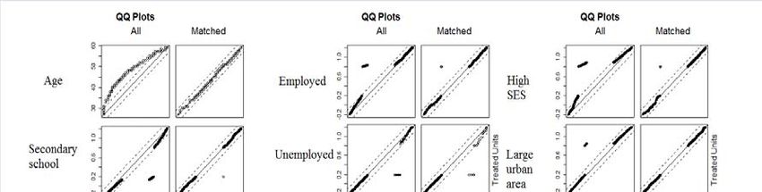
Table 2 shows the after-matching samples which constitute together a sample of 998 females.
The importance of this technique can be illustrated by the professional status at the first
observation (time of diagnosis for cancer survivors) and the professional status two years
after. Only the proportions of the former are similar with around 85% of employed females in
both cancer and general population groups. In addition the proportions of inactive and retired
females are quite similar between the two samples. Although the similar proportions between
groups give account of the effectiveness of the propensity score case-control technique for
balancing the samples, in the figures of the appendix 2a-b we clearly observe that the sample
bias was reduced: we show for example the Quantil-Quantil differences (Q-Q plot in appendix
2a) indicating that the empirical distribution created after the matching procedure is the same
between the diagnosed and the non-diagnosed samples. In fact the Q-Q plots show that the
most part of the points lie on the 45° diagonal. Similarly the figure in the appendix 2b shows
the distribution of the samples before and after the matching process: in fact in the middle of
the figure it is clear to observe that the samples are well balanced.
The proportions observed for the professional status two years after the first interview (or two
years after the diagnosis for breast cancer survivors), show important differences between
groups: there are about 10 percentage points more employed females in the general population
sample (77,6%), whereas on the side of the cancer sample the proportion of the unemployed,
retired and inactive females is relatively more important. These observed differences after the
matching process are, in fact, the phenomenon in which we are interested: the comparison of
the similar groups (in term of the socio-demographic characteristics) suggests that the cancer
diagnosed females move more towards unemployment, inactivity and retirement than their
counterparts in the general population. The remaining question is whether the temporary
separation of the employment (towards unemployment or inactivity) after the breast cancer
diagnosis is more probable than the definitive separation (retirement). In fact, the
improvement of the diagnosis procedures, the prevention methods and the better care
providing extending the life expectancies in that concerning breast cancer make us expect that
the employment separations in the cancer group are mostly temporary. From this perspective,
two emerging questions are: whether the mobility patterns are different between the cancer
survivors and the general population groups; and whether belonging to low or high SES
modifies these patterns.
4Table 1. Individual characteristics comparison before the matching process
Cancer survey Employment survey
N (%) N (%)
Total 595 10211
Age
Mean (sd) 47,8 (6,809) 42,1 (8,74)
25th percentile 44 35
50th percentile 49 42
75th percentile 53 49
Married = 1 415 69,7 7063 69,2
At least one child aged of less than 18 years 192 32,7 5105 50
Education level
Without diploma-primary school 132 22,2 1797 17,6
Secondary school 202 33,9 4802 47
High school 116 19,5 1385 13,6
Higher educationa 145 24,4 2491 21,8
Professional Status at first interview (time of
diagnosis for cancer survivors)
Employed 462 77,6 6960 68,2
Unemployed 33 5,5 778 7,6
Retired 23 3,9 120 1,2
Inactive 77 12,9 2353 23
Professional Status two years later
Employed 365 61,3 6987 68,4
Unemployed 55 9,2 614 6
Retired 49 8,2 216 2,1
Inactive 126 21,2 2393 23,4
SES
Low SES 99 20,0 1701 37,5
High SESb 476 80,0 6384 62,5
Urban size
=100 000 habitants 267 44,9 3971 38,9
a
This category is formed by the following levels: bachelor, master, professional graduate studies, and Ph.D or more.
b
The low SES category includes: farmers, artisans, factory workers, and drivers. The high SES category includes: top executives,
intermediate professionals, and white-collar.
5Table 2. Individual characteristics comparison after the matching process
Cancer survey Employment survey
N (%) N (%)
Total 499 499
Age
Mean (sd) 47,5 (6,67) 47,5 (6,64)
25th percentile 43,0 43,0
50th percentile 49,0 49,0
75th percentile 53,0 53,0
Married = 1 350 70,1 349 69,9
At least one child aged of less than 18 years 161 32,3 162 32,5
Education level
Without diploma-primary school 109 21,8 115 23,0
Secondary school 184 36,9 185 37,1
High school 83 16,6 82 16,4
Higher educationa 123 24,6 122 24,4
Professional Status at first interview (time of
diagnosis for cancer survivors)
Employed 425 85,2 422 84,6
Unemployed 14 2,8 18 3,6
Retired 4 ,8 4 ,8
Inactive 56 11,2 55 11,0
Professional Status two years later
Employed 336 67,3 387 77,6
Unemployed 37 7,4 20 4,0
Retired 25 5,0 15 3,0
Inactive 101 20,2 77 15,4
SES
Low SES 96 19,2 98 19,6
High SESb 403 80,8 401 80,4
Urban size
=100 000 habitants 287 57,5 287 57,5
a
This category is formed by the following levels: bachelor, master, professional graduate studies, and Ph.D or more.
b
The low SES category includes: farmers, artisans, factory workers, and drivers. The high SES category includes: top executives,
intermediate professionals, and white-collar.
63. A continuous-time Markov model for estimating the trajectories in the labor market
In this study where the trajectories of French females are observed in a two-year span, one of
the most important obstacles is that the information between two visits is not available. This is
not an exclusive feature of our data. In fact, labor market surveys are often confronted to
incomplete information (i.e. intermittent follow-up, censored episodes, etc.) It is also difficult
to know the exact history of individuals in the labor market. In order to deal with the obstacles
imposed by the data and assuming that the evolution of the professional status of females only
depends on the state in which they were observed the first time (or at the time of diagnosis for
cancer survivors), we use the continuous-time Markov process estimation.
In a recent work, Bosch and Maloney (2007) use average transition matrices and derivative
statistics to identify and establish stylized facts about labor force dynamics. These authors use
a multi-state model in which individuals can move among five states within the labor market.
A more commonly-used model is the “illness-death” model, with three states that represent
health, illness, and death. In this study, we use an analogous three-state model (see figure 1)
with employment, non-employment (formed by unemployment and inactivity), and retirement
as the three possible states within the labor market2. The final state also acts as the absorbing,
or “death” state. In fact, we assume that individuals in the retirement state never change their
status, which is verified by the data we use.
Figure 1. "Illness-death" model
Employed Non Employed
Retired
Using the Markov chains, we assume that the future evolution only depends on the current
state. If is a homogenous Markov process defined over a discrete state-space equal to
1, … , , where is the number of possible states that a worker could occupy, then the
discrete-time transition matrix is:
, Pr | 0,1,2, … 0,1,2 … (1)
The last equation represents the probability of moving from the state to state in one period
( ). The next state to which the individual moves and the time of the change are governed by
a set of transition intensities , for individual characteristics that do not vary with time,
2 Initially, we specified a model with four states (employment, unemployment, inactivity, and retirement), but
the small number of observations in the inactivity state prevented convergence at the time of the estimation.
Thus, we have decided to merge unemployment and inactivity states in a single state named “non-employment.”
7captured by the variable . The transition intensity matrix is formed by the
instantaneous risk of moving from state to state :
|
, (2)
The two main restrictions are first that the rows of the matrix sum to zero, and second that
its diagonal entries are defined by ∑ . Thus, if ⁄ , the solution is
given by:
(3)
In order to estimate the matrix , Kalbfleisch and Lawless (1985) used a quasi-Newton
algorithm. Their maximum likelihood procedure approach establishes that the inference will
be not reliable if the matrix is not embeddable. In this case, standard asymptotic theory does
not apply3. However, many conditions have been proposed to verify the embeddability of -
matrices. Unfortunately, for multi-state models with more than two states, only the necessary
conditions for the embeddability of are known4. Following Fougère and Kamionka (1992),
once we estimate , we then verify the following properties:
, 1,2,3, ̂ 0; allows 3 values , , , real, positive, different, such as
| | 1, 1,2,3 where are the diagonal entries of the matrix; there is a unique
solution to the equation (3).
Given the objective of this paper, which is to study the impact of a chronic disease on the
mobility between employment, non-employment and retirement, we will introduce a non-
time-varying explanatory variable . The transition intensity matrix elements depend on in
the following way:
exp (4)
The new matrix is then used to determine the statistical likelihood5.
The delta method used in the estimation by maximum of the log-likelihood allows us to
estimate the asymptotic standard errors for the intensity matrix6. However, for , the delta
method cannot be used to obtain standard errors. Additionally, the asymptotic standard errors
are expected to be underestimates of the true standard errors; that is, they act as Cramer-Rao
lower bounds. Therefore, we estimate the different matrices using the bootstrap technique,
3 In practice, there are two main problems in the estimation of the continuous time transition matrix, namely the
aliasing and the embeddability problems. The former implies the impossibility of finding a unique solution for
the equation (3). That means the possible existence of more than one underlying continuous matrix that generates
the observed discrete-time matrix. Secondly, the embeddability problem is in fact the incompatibility between
the theoretical model and the solutions obtained for the matrix ; the elements of the latter must satisfy the
restrictions enumerated above. See singer and Spilerman (1976) and Geweke et al. (1986) for a detailed list of
necessary conditions for the embeddability of .
4 The only necessary and sufficient condition that has been proposed for two-state -matrices is as follows: the
estimation of the transition probability matrix is compatible if and only if the trace of is strictly greater than
one.
5 See the work of Marshall and Jones (1995) for further information about the covariates specification.
6 The estimated variance-covariance matrix is derived by applying the multivariate version of the delta theorem
(Kalbfleisch and Lawless, 1985).
8calculating the bootstrap standard error (Bosch and Maloney, 2007). For that purpose, we
replicate the estimation 10,000 times.
4. Results
In this section we describe the continuous-time Markov process estimations that generated
transition matrices for different groups. First, we present the transition matrix including as
covariate a dummy variable indicating whether the female has or not been diagnosed with
breast cancer. The second part or our results is made using a twice-stratified sample. We first
distinguish diagnosed females from those who are not. Then, we stratify according the low
and high socioeconomic status groups (by SES). Given the objective of this study, in this
section we only present the estimations of the probability transition matrices.
4.1 The impact of the breast cancer diagnosis on the mobility in the labor market
Table 3 shows the estimated probability transition matrices for both diagnosed and non-
diagnosed groups. First of all, we observe that remaining employed within the observed two-
year period is more likely for individuals without cancer. In fact, the probability of being
employed two years after the first observation is around 90% for the non-diagnosed females,
while the chances to remain employed at the end of the observation period is only 78,6% for
females surviving to the breast cancer. In fact, the breast cancer diagnosis seems to induce the
females to leave their employment mostly towards the NE state: the probability of the E-NE
transition two years after the diagnosis is more than 2 times higher than the one observed for
non-diagnosed females. These results suggest that the breast cancer does not induce females
to leave definitively the labor market by the way of the retirement, although retiring is more
probable for diagnosed females (4%) than for non-diagnosed (1,3%). In that concerning the
access into employment, the NE-E transition appears slightly more probable for the females
without breast cancer (8%) than for those diagnosed (5,6%). Nevertheless, the most important
feature concerns the decision of going towards retirement from non-employment (NE-R
transition). Our estimations reveal that the breast cancer diagnosis is not at the origin of an
increase of the probability of retiring. In fact, it is relatively more probable to go towards
retirement for non-diagnosed females (6,8% versus 5% for diagnosed females). The
remaining question is whether the estimated probabilities evolve beyond the 2 years of
observation.
9Table 3. Transition probability matrices for both non-diagnosed and diagnosed females
(Balanced samples: N=998)
No cancer diagnosed Cancer diagnosed
(n=499) (n=499)
Final state 2 years after the first observation
Initial state E NE R E NE R
E 0,904 0,083 0,013 E 0,786 0,173 0,040
0,001 0,001 0,000 0,001 0,001 0,000
NE 0,080 0,851 0,068 NE 0,056 0,894 0,050
0,001 0,002 0,001 0,001 0,002 0,002
R Absorbing state R Absorbing state
Standard errors are in italics.
E: employment, NE: non employment, and R: retirement.
Our bootstrap estimations are based on 10000 replications.
Non employment includes unemployment and inactivity.
One of the advantages of the continuous-time Markov method is that we can use the
estimations based in the observed period to predict the probabilities for future periods.
Assuming that the future social and economic conditions are similar to those at the observed
period, we estimate the transition probabilities for different time’s point in the future. We
carry out this simulation in order to observe ceteris paribus the evolution of the different
transition probabilities for both diagnosed and non-diagnosed groups of individuals.
Figure 2 shows the probabilities of moving between the states considered in this study. The
first column of figures represents the transitions from the employment (E), whereas in the
second column of figures the state of origin is the non-employment (NE). In these figures, the
gap between the lines represents the impact of the breast cancer diagnosis on the different
types of mobility. The probability of remaining employed decreases for both diagnosed and
non-diagnosed groups: in fact, the breast cancer seems to accelerate this reduction. The
situation is similar for the probability of remaining into non-employment although the highest
probabilities are associated to the females diagnosed with breast cancer. The transitions
between E and NE in both directions show similar patterns although the access into
employment is more probable for non-diagnosed females, whereas becoming non-employed is
more probable for females diagnosed with breast cancer. Nevertheless, the transitions between
of the type E-NE show an important feature. The simulated probabilities are increasing until a
given point in time, and then decreases. It seems that in the long run, the breast cancer
survivors and the non-diagnosed females experience similar probabilities of moving between
employment and non-employment. In that concerning the transitions towards retirement, we
observe that two years after diagnosis the probability is similar between both diagnosed and
non-diagnosed groups. Nevertheless, the slope of the curve representing the diagnosed
females becomes more pronounced. That is, the probability of becoming retired is relatively
high for cancer survivors.
Summarizing, the simulated probabilities suggest that the impact of the breast cancer
diagnosis persists in the long run for remaining employed or non-employed as well as for
moving towards retirement: the gap between the corresponding curves persist as the time goes
by. On the contrary, it seems that the effect of the breast cancer diagnosis tends to disappear
in the long run particularly for the E-NE transition. Although the simulated probabilities show
well the impact of the breast cancer diagnosis on the mobility across the different states, it
10seems that the described patterns are mostly related with the socio-demographic
characteristics of individuals. It is important to take into account that the mean age of both the
diagnosed and the non-diagnosed groups is 47,5 years. The simulated probabilities involve an
ageing effect that seems to be dominating the described patterns. These last seems to be
mostly reflecting the life cycle of females in the labor market: that is, the probability of
remaining employed or non-employed converges to zero (individuals leaving the labor
market), and we could expect that the movements between E and NE in both directions will
result in an inverse U-shaped form showing that the labor market becomes less dynamic after
a given point in time. This is confirmed by the pattern of the probabilities of going towards
retirement, which increases monotonically. Our results in this part of the analysis showed that
the breast cancer diagnosis has a negative impact for remaining employed and for returning to
work. Nevertheless, several studies including the one of Spelten et al., (2002) argue that
effectuating manual and physical-demanding activities (low SES) are at the origin of weak
probabilities for remaining employed or for returning to work. From this perspective, we
could expect that belonging to a high SES attenuates the effects of the breast cancer diagnosis
on the probabilities of moving across the considered states (or remaining in the same state).
But, is the effect of high SES enough to erase the one of the breast cancer diagnosis? The
estimations in the next sub-section will shed some light about this fact.
Figure 2. Evolution of the probabilities of moving between employment, non-
employment and retirement
114.2 Breast cancer diagnosis vs. socio-economic status
The table 4 shows the probability matrices estimation for both diagnosed and non-diagnosed
groups stratified according low and high SES. Comparing the groups horizontally, we find the
expected order indicating that the females in the low-SES category are less likely to remain
employed than those in the high-SES category. Nevertheless, the effect of the SES is more
pronounced among the breast cancer diagnosed: the probability of remaining employed for
those in high-SES is 8 percentage points more important than the one for low-SES workers
(within the non-diagnosed groups the difference is only of around 4 percentage points). It is
surprising to observe, on one hand, that the access into employment probability is quite
similar for both low and high SES groups among the cancer diagnosed (around 5,5%). On the
other hand, leaving the employment by recalling into unemployment or inactivity (NE) is
more probable for low-SES workers particularly those diagnosed with breast cancer: for these
last, the probability of effectuating a transition of the type E-NE is 10 percentage points
higher than the one estimated for the diagnosed females in high-SES.
The vertical comparison of the groups in the table 4 shows that the effect of the cancer
diagnosis remains important even by stratifying the samples by SES. Within the low-SES
group, the diagnosed females are much less likely to remain employed (with a probability of
71,6%), than their non-diagnosed counterparts (whose probability is 86,3%). On the contrary,
the former are much more likely to go towards non-employment (26%) than the latter (13%).
In that concerning the non-employed at the initial observation, the cancer diagnosis effect
seems not very important among the low-SES workers. The vertical comparison for the high-
SES group offer similar features.
12Table 4. Transition probability matrices for both non-diagnosed and diagnosed females
(Balanced samples: N=998)
Low SES no cancer diagnosed High SES no Cancer diagnosed
(n=98) (n=401)
Final state 2 years after the first observation
E NE R E NE R
Initial state
E 0,863 0,130 0,007 E 0,908 0,078 0,014
0,003 0,003 0,000 0,001 0,001 0,000
NE 0,067 0,874 0,059 NE 0,099 0,808 0,093
0,003 0,004 0,003 0,003 0,004 0,003
R Absorbing state R Absorbing state
Low SES breast cancer diagnosed High SES breast cancer diagnosed
(n=96) (n=403)
Final state 2 years after the first observation
E NE R E NE R
Initial state
E 0,716 0,261 0,023 E 0,796 0,165 0,039
0,005 0,005 0,002 0,001 0,001 0,001
NE 0,057 0,895 0,048 NE 0,054 0,858 0,088
0,004 0,006 0,004 0,001 0,005 0,004
R Absorbing state R Absorbing state
Standard errors are in italics.
E: employment, NE: non employment, and R: retirement.
Our bootstrap estimations are based on 10000 replications.
Non employment includes unemployment and inactivity.
Although our estimations show that the effect of the SES is the expected one: high-SES
workers remains more into employment and go less towards non-employment, it is difficult to
observe the extent in which the SES attenuates the impact of the cancer diagnosis. In order to
observe this, the figure 3 shows the simulated probabilities for the different groups. First of all
we observe that the most vulnerable group in that concerning the mobility between E and NE
in both directions (and staying in them) is the one of diagnosed females in the low-SES. The
females diagnosed in low-SES are the most (less) likely to remain employed (non-employed).
In that concerning the mobility between the E and NE in both directions, these females
(diagnosed in low-SES) are still the most vulnerable of the labor market. Similarly, the
females not diagnosed in high-SES appear as the group with the best position in the labor
market: easier access to employment, less separation from employment and high (low)
probabilities of remaining employed (non-employed). For remaining employed and moving
from NE to E the cancer diagnosis seems to be the dominating effect. Nevertheless, for
remaining non-employed and moving from E to NE the SES seems to be modifying the effect
of the breast cancer diagnosis. For these cases, the probabilities of diagnosed females but in
high-SES are similar to those of non-diagnosed females but in low-SES. This result points out
that the breast cancer diagnosis is a degrading factor of the situation of high-SES females:
these last are as likely as the low-SES females (not diagnosed) for leaving employment and
for remaining non-employed. Finally, we observe at the bottom of the figure 4 an asymmetric
pattern between the employment and the non-employment in that concerning the transition
13towards retirement. On one hand, the cancer diagnosis effect dominates the one of the SES:
females are more likely to go towards the retirement when the initial state is the employment.
On the other hand, the SES is the dominating effect: the high-SES individuals are more likely
to become retired when the initial state is the non-employment. This result proves that the
breast cancer diagnosis accelerates the process of early retirement for employed survivors.
Figure 3. Evolution of the probabilities of moving between employment, non-
employment and retirement for low and high SES groups
Discussion
In this study, we examined the impact of breast cancer on transitions between employment,
non-employment and retirement two years after diagnosis. Among breast cancer survivors
who were employed at the time of diagnosis, 80% remain at work two years later, which is in
line with previous studies (Maunsell et al. (2004), Bloom et al. (2004), Bushunow et al.
(1995)). This can be explained by the fact that female affected by breast cancer recover a
good health status relatively quickly. This is confirmed by our data which show that the
relative prognosis at the time of diagnosis of breast cancer is 72 (in a scale from 0 to 100).
This is a high relative prognosis if we consider that the one for other types of cancer is from
29 (for lung cancer) to 64 (for prostate cancer). Women diagnosed with breast cancer show
higher transition probabilities of moving from employment to non-employment or retirement
14than females without cancer. Our results are in line with Taskila et al. (2005), who noticed
that unemployment or early retirement was common among people with breast cancer two or
three years after diagnosis; even if the labor situation is worst for those with a highly
disabling cancer of poor prognosis.
We identified some studies using a control group to study unemployment of breast cancer
patients (Taskila et al., (2005); Maunsel et al., (2004); Bradley et al., (2005); Carlsen et al.,
(2008)). However, except the work of Bradley et al., (2005), the case-control matching is
based on two or three individuals’ characteristics. One of the main innovations of this study is
the use of many control variables to create the comparison group. In fact, the introduction of
more socio-demographic characteristics as the criteria to match the two samples increases the
robustness of the final results. Specificity is the use of the continuous-time Markov chains in
this context.
The study of the mobility in the labor market of breast cancer diagnosed females also revealed
that those non-employed at the time of diagnosis were only 4 percentage points more likely to
be in the same state two years after than the non-diagnosed females. These results are in
agreement with the findings of Bradley et al. (2005) who studied persistence of
unemployment among female diagnosed with breast cancer. Nevertheless, the most important
effect of the breast cancer diagnosis among French females is observed on the probability of
remaining employed two years after. This situation persists after distinguishing between low
and high SES particularly for the former.
Our results also show that there is an important incentive for old patients of leaving the labor
force by appealing to their right of early retirement. Nevertheless, the access to the early
retirement reveals an asymmetrical pattern according to the initial state. Employed females
are more likely to retire when they are breast cancer survivors, whereas those non-diagnosed
females are more likely to retire when they are non-employed. The illness event seems to
induce patients to leave the work force especially for high-SES workers. This decision could
either improve or worsen health. In fact, the opinions are divergent: for some authors, early
retirement leads to a better health condition (J.R. Wolfe (1985)), although « physical and
intellectual stimuli of job may improve health » (Mc Garry (2004)). The reason to take early
retirement, as reported by many studies, is explained by poor health. As this explanation is
based on self-reported answers, some authors refer to the "justification bias", i.e. individuals
justify retirement by a health problem because it’s a more socially acceptable explanation,
even if it’s untrue (Campbell and Campbell (1976), J. R. Wolfe (1985)). Early retirement is a
crucial decision because of the financial difficulties coming with the illness. The income loss
is especially increased because breast cancer represents an unexpected change in health.
Without anticipation, the beneficiary will receive a lower retirement income compared with
the one who has planed his early departure and adapted his savings to compensate the future
shortfall (Mc Garry (2004)). Thus early retirement has economical, societal and physical
implications.
Given the importance of socioeconomic status with regard to the probability of job loss,
Taskila-Abrandt et al. (2004) found the largest differences in employment rates among people
working in mining and agriculture, forestry, fishery, transport, and communication, all of
which are mostly manual jobs, as compared with other types of work. This is consistent with
our results. However, we note the difficulty in disentangling whether these observed
systematic differences along socioeconomic statuses are illness-related (such as cancer sites or
severity of the illness) or job-related (such as physical demands). Thanks to our methodology,
15the main contribution of this paper is that a decomposition of both sources of heterogeneity is
now possible. It is well know that the ability to return to work or remaining employed has an
epidemiological basis. Nevertheless, our study contributes principally by demonstrating that
the differences between diagnosed and non-diagnosed females have also an economic
explanation. The probability of being employed two years after diagnosis is the weakest for
low-SES females. This is a net measurement of the relative disadvantage of manual workers
and farmers in returning to work after cancer in contrast to high-SES individuals. In addition
we showed with our estimations that the breast cancer diagnosis is a deteriorating factor of the
conditions that high-SES workers have in the labor market. There are many explanations for
the differences between the SES groups according to their health status –in this case the breast
cancer-. One explanation could be that the French social protection system gives rights to a
replacement income or invalidity pension that could be, at least for low-skilled professionals,
as attractive as returning to work. Another explanation may lie in the fact that workplace
accommodations are especially difficult to make when labor is manual (Molinié, 2006;
Satariano and DeLorenze, 1996). Regardless, the results of this paper suggest that policy-
makers should be specifically concerned about manual workers affected by cancer. Without
attention from policy-makers, both the general employment policy and the health protection
system could be overwhelmed by the phenomenon detailed in this paper. The economic
policy should also screen the situation of high-SES workers in that concerning the separation
from employment. For these females, experiencing a breast cancer episode may result in a
regressing situation which places them at the same level of a low-SES female without cancer.
References
Bloom, JR., Stewart, SL., Chang, S., Banks, PJ, 2004. Then and now: quality of life of young breast cancer
survivors. Psycho-oncology 13, 147-160.
Bradley, C.J., Bednarek HL, (2002). Employment patterns of long term cancer survivors. Psycho-oncology 11,
188-198.
Bradley, C.J., Neumark, D., Bednarek, H.L., Schenk, M., (2005). Short-term effects of breast cancer on labor
market attachment: results from a longitudinal study. Journal of Health Economics, 24(1); 137-160.
Becker, S., Ichino, A. (2002). Estimation of average treatment effects based on propensity scores. The Stata
Journal, 2 (4), 358-377.
Bloom JR, Stewart SL, Chang S, et al. (2004). Then and now: Quality of life of young breast cancer survivors.
Psychooncology 13:147-160.
Bosch, M., Maloney, W., (2007). Comparative analysis of labor market dynamics using Markov processes: an
application to informality. IZA Discussion papers 3038,Institute for the study of labor.
Bushunow PW, Sun Y, Raubertas RF, et al. (1995). Adjuvant chemotherapy does not affect employment in
patients with early-stage breast cancer. J Gen Intern Med 10:73-76.
Carlsen, K., Oksbjerg Dalton, S., Diderichsen, F., Johansen, C., (2008). Risk for unemployment of cancer
survivors A Danish cohort study. European Journal of Cancer, 44(13); 1866-1874.
Chirikos, T.N, Russell-Jacobs, A., Jacobsen P.B, (2002). Functional impairment and the economic consequences
of female breast cancer. Women’s Health 36, 1-20.
16Fougère, D., Kamionka, T., (1992). Un modèle markovien du marché du travail. Annales d’Economie et de
Statistique. 27, 149-188.
Greaves-Otte, J.G., Greaves, J., Kruyt, P.M., Van Leeuwen, O., Van Der Wouden, J.C, Van Der Does, E, (1991).
Problems at social reintegration of long-term cancer survivors. European Journal of Cancer 27, 178-81.
Hoffman, B., (1999). Cancer survivors’ employment and insurance rights: a prime for oncologists. Oncology
(Williston Park)13, 841-6; discussion 846, 849, 852.
Hoffman, B.,2005. Cancer survivors at work: a generation of progress. CA Cancer J Clin 55, 271-80.
Johnson R.W., Davidoff A.J., Perese K., (2003). Health insurance costs and early retirement decisions. Industrial
and Labor Relations.
Kalbfleisch, J.D., Lawless, J.F., (1985). The analysis of panel data under a Markov assumption. Journal of the
American Statistical Association. 80, 863-871.
Maunsell, E., Brisson, C., Dubois, L., Lauzier, S., Fraser, A., (1999). Work problems after breast cancer: an
exploratory qualitative study. Psycho-oncology 8,467-473.
Maunsell E, Drolet M, Brisson J, et al. (2004). Work situation after breast cancer: Results from a population-
based study. J Natl Cancer Inst 96:1813-1822.
McGarry K., (2004). Health and retirement: do changes in health affect retirement expectations? The Journal of
Human Resources.
Schagen, S.B., van Dam, F., Muller, M.J., Boogerd, W., Lindeboom, J., Bruning,P.F, 1999. Cognitive deficits
after postoperative adjuvant chemotherapy for breast carcinoma. Cancer 85, 640-650.
Short, P.F., Vasey, J.J., Tunceli, K, (2005). Employment pathways in a large cohort of adult cancer survivors.
Cancer. 103, 292-301.
Spelten E.R., Spranger, M.A.J., Verbeek, J., (2002). Factors reported to influence the return to work of cancer
survivors: a literature review. Psycho-oncology. 11,124-131.
Taskila-Abrandt,T., Pukkala, E., Martiikainen, R., Karjalainen, A., Hietanen, P., (2005). Employment status of
Finnish cancer patients in 1997. Psychooncology, 14(3); 221-226.
17Appendix 1: Propensity score matching
a) Introduction
The comparison of two groups is often necessary to highlight a particular behavior within a
group of interest. It is current that significant differences appear among the characteristics of
the compared individuals. Therefore, there exists a skew of selection and the inference of the
possible results would be wrong. Similar groups (comparable) are needed: it can be done by
matching individuals of the group of interest with the group used to compare them. Matching
is based on some individual characteristics. A refined method is the creation of a propensity
score to summarize the various characteristics in one single outcome.
b) General aspects of the method
The aim of matching is creating two groups (diagnosed / non-diagnosed) of individuals
closest as possible in term of socioeconomics characteristics. Matching is used to compare
two groups. This technique applies if the control group is larger than the case group. This
technique is more useful when selection depends only on observable characteristics. For
instance, if the matching variable is “to have or not a breast cancer”, constructing pairs only
on socioeconomics variables seems reasonable because the knowledge on the link between
these variables and the risk of having breast cancer is weak. The built sample supposes that
the individuals follow a binomial distribution, i.e. by construction same probability of being
in the interest group and in the group of control. The skew of selection between the two
matched groups is reduced. However, the method of sampling used force the control group
not to be representative of its sample of origin: the results obtained are not representative of
the general population, but allows the comparison with the sample of interest (in our case the
breast cancer diagnosed females).
c) Propensity score (Rosenbaum et Rubin, 1983)
Let i denote the group of breast cancer survivors, and j the group issued from the general
population. The propensity score matching technique consists in the estimation of the
probability of belonging to breast cancer group. This probability can be estimated from a
Logit or Probit specification: the interest is thus to estimate the probabilities and on the
basis of the observed characteristics common to both the breast cancer and the general
population groups. It is important to note that the choice of covariates has to take into
account that the presence of missing values may result in the failure of the matching. In our
study, we chose the “nearest neighbor” algorithm by setting a Caliper criterion equal to
0,0001. That is, the breast cancer-general population pairs will be created if the | |
0,0001. The algorithm is stopped when there are no more possible pairs.
18Appendix 2a.
Appendix 2b.
Distribution of Propensity Scores
Unmatched Treatment Units
Matched Treatment Units
Matched Control Units
Unmatched Control Units
0.0 0.1 0.2 0.3 0.4
Propensity Score
19You can also read