ORB: an efficient alternative to SIFT or SURF
←
→
Page content transcription
If your browser does not render page correctly, please read the page content below
ORB: an efficient alternative to SIFT or SURF

               Ethan Rublee              Vincent Rabaud                Kurt Konolige              Gary Bradski
                                              Willow Garage, Menlo Park, California
                           {erublee}{vrabaud}{konolige}{bradski}@willowgarage.com

                         Abstract

   Feature matching is at the base of many computer vi-
sion problems, such as object recognition or structure from
motion. Current methods rely on costly descriptors for de-
tection and matching. In this paper, we propose a very fast
binary descriptor based on BRIEF, called ORB, which is
rotation invariant and resistant to noise. We demonstrate
                                                                     Figure 1. Typical matching result using ORB on real-world im-
through experiments how ORB is at two orders of magni-
                                                                     ages with viewpoint change. Green lines are valid matches; red
tude faster than SIFT, while performing as well in many              circles indicate unmatched points.
situations. The efficiency is tested on several real-world ap-
plications, including object detection and patch-tracking on
a smart phone.                                                       FAST and Rotated BRIEF). Both these techniques are at-
                                                                     tractive because of their good performance and low cost.
                                                                     In this paper, we address several limitations of these tech-
1. Introduction                                                      niques vis-a-vis SIFT, most notably the lack of rotational
                                                                     invariance in BRIEF. Our main contributions are:
    The SIFT keypoint detector and descriptor [17], al-
though over a decade old, have proven remarkably success-              • The addition of a fast and accurate orientation compo-
ful in a number of applications using visual features, in-               nent to FAST.
cluding object recognition [17], image stitching [28], visual          • The efficient computation of oriented BRIEF features.
mapping [25], etc. However, it imposes a large computa-
                                                                       • Analysis of variance and correlation of oriented
tional burden, especially for real-time systems such as vi-
                                                                         BRIEF features.
sual odometry, or for low-power devices such as cellphones.
This has led to an intensive search for replacements with              • A learning method for de-correlating BRIEF features
lower computation cost; arguably the best of these is SURF               under rotational invariance, leading to better perfor-
[2]. There has also been research aimed at speeding up the               mance in nearest-neighbor applications.
computation of SIFT, most notably with GPU devices [26].
                                                                        To validate ORB, we perform experiments that test the
    In this paper, we propose a computationally-efficient re-
                                                                     properties of ORB relative to SIFT and SURF, for both
placement to SIFT that has similar matching performance,
                                                                     raw matching ability, and performance in image-matching
is less affected by image noise, and is capable of being used
                                                                     applications. We also illustrate the efficiency of ORB
for real-time performance. Our main motivation is to en-
                                                                     by implementing a patch-tracking application on a smart
hance many common image-matching applications, e.g., to
                                                                     phone. An additional benefit of ORB is that it is free from
enable low-power devices without GPU acceleration to per-
                                                                     the licensing restrictions of SIFT and SURF.
form panorama stitching and patch tracking, and to reduce
the time for feature-based object detection on standard PCs.
                                                                     2. Related Work
Our descriptor performs as well as SIFT on these tasks (and
better than SURF), while being almost two orders of mag-             Keypoints FAST and its variants [23, 24] are the method
nitude faster.                                                       of choice for finding keypoints in real-time systems that
    Our proposed feature builds on the well-known FAST               match visual features, for example, Parallel Tracking and
keypoint detector [23] and the recently-developed BRIEF              Mapping [13]. It is efficient and finds reasonable corner
descriptor [6]; for this reason we call it ORB (Oriented             keypoints, although it must be augmented with pyramid

                                                                 1
schemes for scale [14], and in our case, a Harris corner filter   We use FAST-9 (circular radius of 9), which has good per-
[11] to reject edges and provide a reasonable score.              formance.
   Many keypoint detectors include an orientation operator            FAST does not produce a measure of cornerness, and we
(SIFT and SURF are two prominent examples), but FAST              have found that it has large responses along edges. We em-
does not. There are various ways to describe the orientation      ploy a Harris corner measure [11] to order the FAST key-
of a keypoint; many of these involve histograms of gradient       points. For a target number N of keypoints, we first set the
computations, for example in SIFT [17] and the approxi-           threshold low enough to get more than N keypoints, then
mation by block patterns in SURF [2]. These methods are           order them according to the Harris measure, and pick the
either computationally demanding, or in the case of SURF,         top N points.
yield poor approximations. The reference paper by Rosin               FAST does not produce multi-scale features. We employ
[22] gives an analysis of various ways of measuring orienta-      a scale pyramid of the image, and produce FAST features
tion of corners, and we borrow from his centroid technique.       (filtered by Harris) at each level in the pyramid.
Unlike the orientation operator in SIFT, which can have
                                                                  3.2. Orientation by Intensity Centroid
multiple value on a single keypoint, the centroid operator
gives a single dominant result.                                      Our approach uses a simple but effective measure of cor-
                                                                  ner orientation, the intensity centroid [22]. The intensity
Descriptors BRIEF [6] is a recent feature descriptor that         centroid assumes that a corner’s intensity is offset from its
uses simple binary tests between pixels in a smoothed image       center, and this vector may be used to impute an orientation.
patch. Its performance is similar to SIFT in many respects,       Rosin defines the moments of a patch as:
including robustness to lighting, blur, and perspective dis-
                                                                                            X
                                                                                     mpq =      xp y q I(x, y),             (1)
tortion. However, it is very sensitive to in-plane rotation.                                x,y
    BRIEF grew out of research that uses binary tests to
train a set of classification trees [4]. Once trained on a set    and with these moments we may find the centroid:
of 500 or so typical keypoints, the trees can be used to re-
                                                                                           m10 m01

turn a signature for any arbitrary keypoint [5]. In a similar                       C=        ,                            (2)
                                                                                           m00 m00
manner, we look for the tests least sensitive to orientation.
The classic method for finding uncorrelated tests is Princi-      We can construct a vector from the corner’s center, O, to the
pal Component Analysis; for example, it has been shown                       ~ The orientation of the patch then simply is:
                                                                  centroid, OC.
that PCA for SIFT can help remove a large amount of re-
                                                                                    θ = atan2(m01 , m10 ),                 (3)
dundant information [12]. However, the space of possible
binary tests is too big to perform PCA and an exhaustive          where atan2 is the quadrant-aware version of arctan. Rosin
search is used instead.                                           mentions taking into account whether the corner is dark or
   Visual vocabulary methods [21, 27] use offline clustering      light; however, for our purposes we may ignore this as the
to find exemplars that are uncorrelated and can be used in        angle measures are consistent regardless of the corner type.
matching. These techniques might also be useful in finding           To improve the rotation invariance of this measure we
uncorrelated binary tests.                                        make sure that moments are computed with x and y re-
   The closest system to ORB is [3], which proposes a             maining within a circular region of radius r. We empirically
multi-scale Harris keypoint and oriented patch descriptor.        choose r to be the patch size, so that that x and y run from
This descriptor is used for image stitching, and shows good       [−r, r]. As |C| approaches 0, the measure becomes unsta-
rotational and scale invariance. It is not as efficient to com-   ble; with FAST corners, we have found that this is rarely the
pute as our method, however.                                      case.
                                                                     We compared the centroid method with two gradient-
3. oFAST: FAST Keypoint Orientation                               based measures, BIN and MAX. In both cases, X and
                                                                  Y gradients are calculated on a smoothed image. MAX
    FAST features are widely used because of their compu-         chooses the largest gradient in the keypoint patch; BIN
tational properties. However, FAST features do not have an        forms a histogram of gradient directions at 10 degree inter-
orientation component. In this section we add an efficiently-     vals, and picks the maximum bin. BIN is similar to the SIFT
computed orientation.                                             algorithm, although it picks only a single orientation. The
                                                                  variance of the orientation in a simulated dataset (in-plane
3.1. FAST Detector
                                                                  rotation plus added noise) is shown in Figure 2. Neither of
   We start by detecting FAST points in the image. FAST           the gradient measures performs very well, while the cen-
takes one parameter, the intensity threshold between the          troid gives a uniformly good orientation, even under large
center pixel and those in a circular ring about the center.       image noise.
Standard Deviation in Angle Error Histogram of Descriptor Bit Mean Values
40
BRIEF
Standard Deviation (degrees)
35 140 rBRIEF
steered BRIEF
30
120
25
20
100
15
IC
Number of Bits
MAX
10 BIN 80
5
0 5 10 15 20 25
Image Intensity Noise (gaussian noise for an 8 bit image) 60
Figure 2. Rotation measure. The intensity centroid (IC) per- 40
forms best on recovering the orientation of artificially rotated noisy
20
patches, compared to a histogram (BIN) and MAX method.
0
0
0.
0.
0.
0.
0.
0.
0.
0.
0.
0.
05
1
15
2
25
3
35
4
45
5
Bit Response Mean
4. rBRIEF: Rotation-Aware Brief
Figure 3. Distribution of means for feature vectors: BRIEF, steered
In this section, we first introduce a steered BRIEF de- BRIEF (Section 4.1), and rBRIEF (Section 4.3). The X axis is the
scriptor, show how to compute it efficiently and demon- distance to a mean of 0.5
strate why it actually performs poorly with rotation. We
then introduce a learning step to find less correlated binary but this solution is obviously expensive. A more efficient
tests leading to the better descriptor rBRIEF, for which we method is to steer BRIEF according to the orientation of
offer comparisons to SIFT and SURF. keypoints. For any feature set of n binary tests at location
(xi , yi ), define the 2 × n matrix
4.1. Efficient Rotation of the BRIEF Operator
Brief overview of BRIEF x1 , . . . , xn
S=
y1 , . . . , yn
The BRIEF descriptor [6] is a bit string description of an
image patch constructed from a set of binary intensity tests. Using the patch orientation θ and the corresponding rotation
Consider a smoothed image patch, p. A binary test τ is matrix Rθ , we construct a “steered” version Sθ of S:
defined by:
Sθ = Rθ S,
1 : p(x) < p(y)
τ (p; x, y) := , (4) Now the steered BRIEF operator becomes
0 : p(x) ≥ p(y)
gn (p, θ) := fn (p)|(xi , yi ) ∈ Sθ (6)
where p(x) is the intensity of p at a point x. The feature is
defined as a vector of n binary tests: We discretize the angle to increments of 2π/30 (12 de-
X grees), and construct a lookup table of precomputed BRIEF
fn (p) := 2i−1 τ (p; xi , yi ) (5) patterns. As long at the keypoint orientation θ is consistent
1≤i≤n
across views, the correct set of points Sθ will be used to
Many different types of distributions of tests were consid- compute its descriptor.
ered in [6]; here we use one of the best performers, a Gaus- 4.2. Variance and Correlation
sian distribution around the center of the patch. We also
choose a vector length n = 256. One of the pleasing properties of BRIEF is that each bit
It is important to smooth the image before performing feature has a large variance and a mean near 0.5. Figure 3
the tests. In our implementation, smoothing is achieved us- shows the spread of means for a typical Gaussian BRIEF
ing an integral image, where each test point is a 5 × 5 sub- pattern of 256 bits over 100k sample keypoints. A mean
window of a 31 × 31 pixel patch. These were chosen from of 0.5 gives the maximum sample variance 0.25 for a bit
our own experiments and the results in [6]. feature. On the other hand, once BRIEF is oriented along
the keypoint direction to give steered BRIEF, the means are
shifted to a more distributed pattern (again, Figure 3). One
Steered BRIEF
way to understand this is that the oriented corner keypoints
We would like to allow BRIEF to be invariant to in-plane present a more uniform appearance to binary tests.
rotation. Matching performance of BRIEF falls off sharply High variance makes a feature more discriminative, since
for in-plane rotation of more than a few degrees (see Figure it responds differentially to inputs. Another desirable prop-
7). Calonder [6] suggests computing a BRIEF descriptor erty is to have the tests uncorrelated, since then each test
for a set of rotations and perspective warps of each patch, will contribute to the result. To analyze the correlation and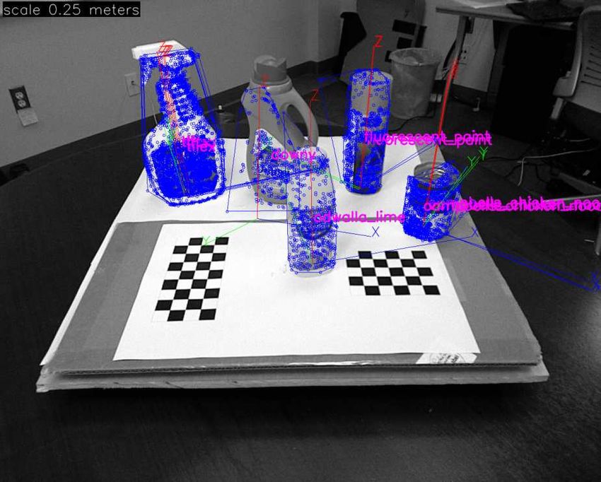
8 large set of binary tests, identify 256 new features that have
BRIEF
Steered BRIEF high variance and are uncorrelated over a large training set.
6 rBRIEF
However, since the new features are composed from a larger
Eigenvalue
4 number of binary tests, they would be less efficient to com-
pute than steered BRIEF. Instead, we search among all pos-
2 sible binary tests to find ones that both have high variance
(and means close to 0.5), as well as being uncorrelated.
0
0 5 10 15 20
Component
25 30 35 40
The method is as follows. We first set up a training set of
Figure 4. Distribution of eigenvalues in the PCA decomposition some 300k keypoints, drawn from images in the PASCAL
over 100k keypoints of three feature vectors: BRIEF, steered 2006 set [8]. We also enumerate all possible binary tests
BRIEF (Section 4.1), and rBRIEF (Section 4.3). drawn from a 31×31 pixel patch. Each test is a pair of 5×5
sub-windows of the patch. If we note the width of our patch
Distance Distribution as wp = 31 and the width of the test sub-window as wt = 5,
0.04
rBRIEF
steered BRIEF
then we have N = (wp − wt )2 possible sub-windows. We
BRIEF
0.035
would like to select pairs of two from these, so we have N2
0.03 binary tests. We eliminate tests that overlap, so we end up
with M = 205590 possible tests. The algorithm is:
Relative Frequency
0.025
0.02 1. Run each test against all training patches.
0.015
2. Order the tests by their distance from a mean of 0.5,
0.01 forming the vector T.
0.005 3. Greedy search:
0
0 64 128 192 256
(a) Put the first test into the result vector R and re-
Descriptor Distance
move it from T.
Figure 5. The dotted lines show the distances of a keypoint to out- (b) Take the next test from T, and compare it against
liers, while the solid lines denote the distances only between inlier
all tests in R. If its absolute correlation is greater
matches for three feature vectors: BRIEF, steered BRIEF (Section
4.1), and rBRIEF (Section 4.3).
than a threshold, discard it; else add it to R.
(c) Repeat the previous step until there are 256 tests
in R. If there are fewer than 256, raise the thresh-
variance of tests in the BRIEF vector, we looked at the re- old and try again.
sponse to 100k keypoints for BRIEF and steered BRIEF.
The results are shown in Figure 4. Using PCA on the data, This algorithm is a greedy search for a set of uncorrelated
we plot the highest 40 eigenvalues (after which the two de- tests with means near 0.5. The result is called rBRIEF.
scriptors converge). Both BRIEF and steered BRIEF ex- rBRIEF has significant improvement in the variance and
hibit high initial eigenvalues, indicating correlation among correlation over steered BRIEF (see Figure 4). The eigen-
the binary tests – essentially all the information is contained values of PCA are higher, and they fall off much less
in the first 10 or 15 components. Steered BRIEF has signif- quickly. It is interesting to see the high-variance binary tests
icantly lower variance, however, since the eigenvalues are produced by the algorithm (Figure 6). There is a very pro-
lower, and thus is not as discriminative. Apparently BRIEF nounced vertical trend in the unlearned tests (left image),
depends on random orientation of keypoints for good per- which are highly correlated; the learned tests show better
formance. Another view of the effect of steered BRIEF is diversity and lower correlation.
shown in the distance distributions between inliers and out-
liers (Figure 5). Notice that for steered BRIEF, the mean for 4.4. Evaluation
outliers is pushed left, and there is more of an overlap with We evaluate the combination of oFAST and rBRIEF,
the inliers. which we call ORB, using two datasets: images with syn-
thetic in-plane rotation and added Gaussian noise, and a
4.3. Learning Good Binary Features
real-world dataset of textured planar images captured from
To recover from the loss of variance in steered BRIEF, different viewpoints. For each reference image, we compute
and to reduce correlation among the binary tests, we de- the oFAST keypoints and rBRIEF features, targeting 500
velop a learning method for choosing a good subset of bi- keypoints per image. For each test image (synthetic rotation
nary tests. One possible strategy is to use PCA or some or real-world viewpoint change), we do the same, then per-
other dimensionality-reduction method, and starting from a form brute-force matching to find the best correspondence.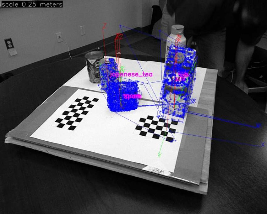
Comparison of SIFT and rBRIEF considering Gaussian Intensity Noise
100
rBRIEF
95 SIFT
90
85
80
Percentage of Inliers
75
70
65
60
55
50
45
40
Figure 6. A subset of the binary tests generated by considering 35
90 180 270 360
high-variance under orientation (left) and by running the learning Angle of Rotation (Degrees)
algorithm to reduce correlation (right). Note the distribution of the Figure 8. Matching behavior under noise for SIFT and rBRIEF.
tests around the axis of the keypoint orientation, which is pointing The noise levels are 0, 5, 10, 15, 20, and 25. SIFT performance
up. The color coding shows the maximum pairwise correlation of degrades rapidly, while rBRIEF is relatively unaffected.
each test, with black and purple being the lowest. The learned tests
clearly have a better distribution and lower correlation.
Percentage of Inliers considering In Plane Rotation
100 rBRIEF
SIFT
SURF
BRIEF
80
Percentage of Inliers
60
40
Figure 9. Real world data of a table full of magazines and an out-
20
door scene. The images in the first column are matched to those in
the second. The last column is the resulting warp of the first onto
the second.
0
0 45 90 135 180 225 270 315 360
Angle of Rotation (Degrees)
Figure 7. Matching performance of SIFT, SURF, BRIEF with we measure the performance of ORB relative to SIFT and
FAST, and ORB (oFAST +rBRIEF) under synthetic rotations SURF. The test is performed in the following manner:
with Gaussian noise of 10.
1. Pick a reference view V0 .
2. For all Vi , find a homographic warp Hi0 that maps
The results are given in terms of the percentage of correct
Vi → V0 .
matches, against the angle of rotation.
Figure 7 shows the results for the synthetic test set with 3. Now, use the Hi0 as ground truth for descriptor
added Gaussian noise of 10. Note that the standard BRIEF matches from SIFT, SURF, and ORB.
operator falls off dramatically after about 10 degrees. SIFT inlier % N points
outperforms SURF, which shows quantization effects at 45- Magazines
degree angles due to its Haar-wavelet composition. ORB
ORB 36.180 548.50
has the best performance, with over 70% inliers.
SURF 38.305 513.55
ORB is relatively immune to Gaussian image noise, un- SIFT 34.010 584.15
like SIFT. If we plot the inlier performance vs. noise, SIFT
Boat
exhibits a steady drop of 10% with each additional noise
ORB 45.8 789
increment of 5. ORB also drops, but at a much lower rate
SURF 28.6 795
(Figure 8).
SIFT 30.2 714
To test ORB on real-world images, we took two sets of
images, one our own indoor set of highly-textured mag- ORB outperforms SIFT and SURF on the outdoor dataset.
azines on a table (Figure 9), the other an outdoor scene. It is about the same on the indoor set; [6] noted that blob-
The datasets have scale, viewpoint, and lighting changes. detection keypoints like SIFT tend to be better on graffiti-
Running a simple inlier/outlier test on this set of images, type images.106 103
105 Caltech 101 - BRIEF
Caltech 101 - steered BRIEF
Query time per feature (ms)
4
10 Caltech 101 - rBRIEF
103
102
102
101
100 0 20 40 60 80 100 120 140 160 180 200 220 240 260 280 300 320 340
Number of buckets
106
105 Pascal 2009 - BRIEF
Pascal 2009 - steered BRIEF 101
104 Pascal 2009 - rBRIEF
3
10
102 rBRIEF
steered BRIEF
101 SIFT
100 0 400 800 1200 1600 2000 2400 2800 3200 3600 4000 4400 4800 100 20 40 60 80 100
Bucket size Success percentage
Figure 10. Two different datasets (7818 images from the PASCAL Figure 11. Speed vs. accuracy. The descriptors are tested on
2009 dataset [9] and 9144 low resolution images from the Caltech warped versions of the images they were trained on. We used 1,
101 [29]) are used to train LSH on the BRIEF, steered BRIEF and 2 and 3 kd-trees for SIFT (the autotuned FLANN kd-tree gave
rBRIEF descriptors. The training takes less than 2 minutes and worse performance), 4 to 20 hash tables for rBRIEF and 16 to 40
is limited by the disk IO. rBRIEF gives the most homogeneous tables for steered BRIEF (both with a sub-signature of 16 bits).
buckets by far, thus improving the query speed and accuracy. Nearest neighbors were searched over 1.6M entries for SIFT and
1.8M entries for rBRIEF.
5. Scalable Matching of Binary Features
the data. As shown in Figure 10, buckets are much smaller
In this section we show that ORB outperforms in average compared to steered BRIEF or normal BRIEF.
SIFT/SURF in nearest-neighbor matching over large
5.3. Evaluation
databases of images. A critical part of ORB is the recovery
of variance, which makes NN search more efficient. We compare the performance of rBRIEF LSH with kd-
trees of SIFT features using FLANN [20]. We train the dif-
5.1. Locality Sensitive Hashing for rBrief ferent descriptors on the Pascal 2009 dataset and test them
on sampled warped versions of those images using the same
As rBRIEF is a binary pattern, we choose Locality Sen-
affine transforms as in [1].
sitive Hashing [10] as our nearest neighbor search. In LSH,
Our multi-probe LSH uses bitsets to speedup the pres-
points are stored in several hash tables and hashed in differ-
ence of keys in the hash maps. It also computes the Ham-
ent buckets. Given a query descriptor, its matching buckets
ming distance between two descriptors using an SSE 4.2
are retrieved and its elements compared using a brute force
optimized popcount.
matching. The power of that technique lies in its ability
Figure 11 establishes a correlation between the speed
to retrieve nearest neighbors with a high probability given
and the accuracy of kd-trees with SIFT (SURF is equiv-
enough hash tables.
alent) and LSH with rBRIEF. A successful match of the
For binary features, the hash function is simply a subset
test image occurs when more than 50 descriptors are found
of the signature bits: the buckets in the hash tables contain
in the correct database image. We notice that LSH is faster
descriptors with a common sub-signature. The distance is
than the kd-trees, most likely thanks to its simplicity and the
the Hamming distance.
speed of the distance computation. LSH also gives more
We use multi-probe LSH [18] which improves on the flexibility with regard to accuracy, which can be interesting
traditional LSH by looking at neighboring buckets in which in bag-of-feature approaches [21, 27]. We can also notice
a query descriptor falls. While this could result in more that the steered BRIEF is much slower due to its uneven
matches to check, it actually allows for a lower number of buckets.
tables (and thus less RAM usage) and a longer sub-signature
and therefore smaller buckets. 6. Applications
5.2. Correlation and Leveling 6.1. Benchmarks
rBRIEF improves the speed of LSH by making the One emphasis for ORB is the efficiency of detection and
buckets of the hash tables more even: as the bits are less description on standard CPUs. Our canonical ORB detec-
correlated, the hash function does a better job at partitioning tor uses the oFAST detector and rBRIEF descriptor, eachcomputed separately
√ on five scales of the image, with a scal-
ing factor of 2. We used an area-based interpolation for
efficient decimation.
The ORB system breaks down into the following times
per typical frame of size 640x480. The code was executed
in a single thread running on an Intel i7 2.8 GHz processor:
ORB: Pyramid oFAST rBRIEF
Time (ms) 4.43 8.68 2.12
When computing ORB on a set of 2686 images at 5
scales, it was able to detect and compute over 2 × 10⁶ fea-
tures in 42 seconds. Comparing to SIFT and SURF on the
same data, for the same number of features (roughly 1000),
and the same number of scales, we get the following times:
Detector ORB SURF SIFT
Time per frame (ms) 15.3 217.3 5228.7
These times were averaged over 24 640x480 images from
the Pascal dataset [9]. ORB is an order of magnitude faster
than SURF, and over two orders faster than SIFT.
6.2. Textured object detection
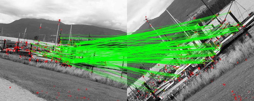
We apply rBRIEF to object recognition by implement- Figure 12. Two images of our textured obejct recognition with
ing a conventional object recognition pipeline similar to pose estimation. The blue features are the training features super-
imposed on the query image to indicate that the pose of the object
[19]: we first detect oFAST features and rBRIEF de-
was found properly. Axes are also displayed for each object as
scriptors, match them to our database, and then perform
well as a pink label. Top image misses two objects; all are found
PROSAC [7] and EPnP [16] to have a pose estimate. in the bottom one.
Our database contains 49 household objects, each taken
under 24 views with a 2D camera and a Kinect device from
Microsoft. The testing data consists of 2D images of sub- While there are real-time feature trackers that can run on
sets of those same objects under different view points and a cellphone [15], they usually operate on very small images
occlusions. To have a match, we require that descriptors are (e.g., 120x160) and with very few features. Systems com-
matched but also that a pose can be computed. In the end, parable to ours [30] typically take over 1 second per image.
our pipeline retrieves 61% of the objects as shown in Figure We were able to run ORB with 640 × 480 resolution at 7
12. Hz on a cellphone with a 1GHz ARM chip and 512 MB of
The algorithm handles a database of 1.2M descriptors RAM. The OpenCV port for Android was used for the im-
in 200MB and has timings comparable to what we showed plementation. These are benchmarks for about 400 points
earlier (14 ms for detection and 17ms for LSH matching in per image:
average). The pipeline could be sped up considerably by not
matching all the query descriptors to the training data but ORB Matching H Fit
our goal was only to show the feasibility of object detection Time (ms) 66.6 72.8 20.9
with ORB.
7. Conclusion
6.3. Embedded real-time feature tracking
In this paper, we have defined a new oriented descrip-
Tracking on the phone involves matching the live frames tor, ORB, and demonstrated its performance and efficiency
to a previously captured keyframe. Descriptors are stored relative to other popular features. The investigation of vari-
with the keyframe, which is assumed to contain a planar ance under orientation was critical in constructing ORB
surface that is well textured. We run ORB on each incom- and de-correlating its components, in order to get good per-
ing frame, and proced with a brute force descriptor match- formance in nearest-neighbor applications. We have also
ing against the keyframe. The putative matches from the contributed a BSD licensed implementation of ORB to the
descriptor distance are used in a PROSAC best fit homog- community, via OpenCV 2.3.
raphy H. One of the issues that we have not adequately addressedhere is scale invariance. Although we use a pyramid scheme national Symposium on Mixed and Augmented Reality (IS-
for scale, we have not explored per keypoint scale from MAR’07), Nara, Japan, November 2007. 1
depth cues, tuning the number of octaves, etc.. Future work [14] G. Klein and D. Murray. Improving the agility of keyframe-
also includes GPU/SSE optimization, which could improve based SLAM. In European Conference on Computer Vision,
LSH by another order of magnitude. 2008. 2
[15] G. Klein and D. Murray. Parallel tracking and mapping on a
camera phone. In Proc. Eigth IEEE and ACM International
References Symposium on Mixed and Augmented Reality (ISMAR’09),
[1] M. Aly, P. Welinder, M. Munich, and P. Perona. Scaling Orlando, October 2009. 7
object recognition: Benchmark of current state of the art [16] V. Lepetit, F. Moreno-Noguer, and P. Fua. EPnP: An accurate
techniques. In First IEEE Workshop on Emergent Issues in O(n) solution to the pnp problem. Int. J. Comput. Vision,
Large Amounts of Visual Data (WS-LAVD), IEEE Interna- 81:155–166, February 2009. 7
tional Conference on Computer Vision (ICCV), September [17] D. G. Lowe. Distinctive image features from scale-invariant
2009. 6 keypoints. International Journal of Computer Vision,
[2] H. Bay, T. Tuytelaars, and L. Van Gool. Surf: Speeded up ro- 60(2):91–110, 2004. 1, 2
bust features. In European Conference on Computer Vision, [18] Q. Lv, W. Josephson, Z. Wang, M. Charikar, and K. Li.
May 2006. 1, 2 Multi-probe LSH: efficient indexing for high-dimensional
[3] M. Brown, S. Winder, and R. Szeliski. Multi-image match- similarity search. In Proceedings of the 33rd international
ing using multi-scale oriented patches. In Computer Vision conference on Very large data bases, VLDB ’07, pages 950–
and Pattern Recognition, pages 510–517, 2005. 2 961. VLDB Endowment, 2007. 6
[4] M. Calonder, V. Lepetit, and P. Fua. Keypoint signatures for [19] M. Martinez, A. Collet, and S. S. Srinivasa. MOPED:
fast learning and recognition. In European Conference on A Scalable and low Latency Object Recognition and Pose
Computer Vision, 2008. 2 Estimation System. In IEEE International Conference on
[5] M. Calonder, V. Lepetit, K. Konolige, P. Mihelich, and Robotics and Automation. IEEE, 2010. 7
P. Fua. High-speed keypoint description and matching us- [20] M. Muja and D. G. Lowe. Fast approximate nearest neigh-
ing dense signatures. In Under review, 2009. 2 bors with automatic algorithm configuration. VISAPP, 2009.
[6] M. Calonder, V. Lepetit, C. Strecha, and P. Fua. Brief: Bi- 6
nary robust independent elementary features. In In European [21] D. Nistér and H. Stewénius. Scalable recognition with a vo-
Conference on Computer Vision, 2010. 1, 2, 3, 5 cabulary tree. In CVPR, 2006. 2, 6
[7] O. Chum and J. Matas. Matching with PROSAC - pro- [22] P. L. Rosin. Measuring corner properties. Computer Vision
gressive sample consensus. In C. Schmid, S. Soatto, and and Image Understanding, 73(2):291 – 307, 1999. 2
C. Tomasi, editors, Proc. of Conference on Computer Vision [23] E. Rosten and T. Drummond. Machine learning for high-
and Pattern Recognition (CVPR), volume 1, pages 220–226, speed corner detection. In European Conference on Com-
Los Alamitos, USA, June 2005. IEEE Computer Society. 7 puter Vision, volume 1, 2006. 1
[8] M. Everingham. The PASCAL Visual Ob- [24] E. Rosten, R. Porter, and T. Drummond. Faster and bet-
ject Classes Challenge 2006 (VOC2006) Results. ter: A machine learning approach to corner detection. IEEE
http://pascallin.ecs.soton.ac.uk/challenges/VOC/databases.html. Trans. Pattern Analysis and Machine Intelligence, 32:105–
4 119, 2010. 1
[9] M. Everingham, L. Van Gool, C. K. I. Williams, J. Winn, [25] S. Se, D. Lowe, and J. Little. Mobile robot localization and
and A. Zisserman. The PASCAL Visual Object Classes mapping with uncertainty using scale-invariant visual land-
Challenge 2009 (VOC2009) Results. http://www.pascal- marks. International Journal of Robotic Research, 21:735–
network.org/challenges/VOC/voc2009/workshop/index.html. 758, August 2002. 1
6, 7 [26] S. N. Sinha, J. michael Frahm, M. Pollefeys, and Y. Genc.
Gpu-based video feature tracking and matching. Technical
[10] A. Gionis, P. Indyk, and R. Motwani. Similarity search in
report, In Workshop on Edge Computing Using New Com-
high dimensions via hashing. In M. P. Atkinson, M. E. Or-
modity Architectures, 2006. 1
lowska, P. Valduriez, S. B. Zdonik, and M. L. Brodie, editors,
VLDB’99, Proceedings of 25th International Conference on [27] J. Sivic and A. Zisserman. Video google: A text retrieval
Very Large Data Bases, September 7-10, 1999, Edinburgh, approach to object matching in videos. International Con-
Scotland, UK, pages 518–529. Morgan Kaufmann, 1999. 6 ference on Computer Vision, page 1470, 2003. 2, 6
[28] N. Snavely, S. M. Seitz, and R. Szeliski. Skeletal sets for
[11] C. Harris and M. Stephens. A combined corner and edge
efficient structure from motion. In Proc. Computer Vision
detector. In Alvey Vision Conference, pages 147–151, 1988.
and Pattern Recognition, 2008. 1
2
[29] G. Wang, Y. Zhang, and L. Fei-Fei. Using dependent regions
[12] Y. Ke and R. Sukthankar. Pca-sift: A more distinctive rep-
for object categorization in a generative framework, 2006. 6
resentation for local image descriptors. In Computer Vision
[30] A. Weimert, X. Tan, and X. Yang. Natural feature detection
and Pattern Recognition, pages 506–513, 2004. 2
on mobile phones with 3D FAST. Int. J. of Virtual Reality,
[13] G. Klein and D. Murray. Parallel tracking and mapping for
9:29–34, 2010. 7
small AR workspaces. In Proc. Sixth IEEE and ACM Inter-You can also read