Coronal Magnetic Field Topology From Total Solar Eclipse Observations
←
→
Page content transcription
If your browser does not render page correctly, please read the page content below
Coronal Magnetic Field Topology From Total Solar Eclipse Observations
                                                                         Benjamin Boe1 , Shadia Habbal1 , and Miloslav Druckmüller2
                                                                          1
                                                                           Institute for Astronomy, University of Hawaii, Honolulu, HI 96822, USA
                                                      2
                                                          Faculty of Mechanical Engineering, Brno University of Technology, Technick 2, 616 69 Brno, Czech Republic
arXiv:2004.08970v1 [astro-ph.SR] 19 Apr 2020

                                                                                                     April 21, 2020

                                                                                                         Abstract
                                                        Measuring the global magnetic field of the solar corona remains exceptionally challenging. The fine-
                                                    scale density structures observed in white light images taken during Total Solar Eclipses (TSEs) are
                                                    currently the best proxy for inferring the magnetic field direction in the corona from the solar limb out
                                                    to several solar radii (R ). We present, for the first time, the topology of the coronal magnetic field
                                                    continuously between 1 and 6 R , as quantitatively inferred with the Rolling Hough Transform (RHT)
                                                    for 14 unique eclipse coronae that span almost two complete solar cycles. We find that the direction of the
                                                    coronal magnetic field does not become radial until at least 3 R , with a high variance between 1.5 and
                                                    3 R at different latitudes and phases of the solar cycle. We find that the most non-radial coronal field
                                                    topologies occur above regions with weaker magnetic field strengths in the photosphere, while stronger
                                                    photospheric fields are associated with highly radial field lines in the corona. In addition, we find an
                                                    abundance of field lines which extend continuously from the solar surface out to several solar radii at
                                                    all latitudes, regardless of the presence of coronal holes. These results have implications for testing and
                                                    constraining coronal magnetic field models, and for linking in situ solar wind measurements to their
                                                    sources at the Sun.

                                               1    Introduction
                                               The shape of the solar corona was first characterized during Total Solar Eclipses (TSE) with hand-drawn sketches
                                               and early photographic techniques (e.g. Maunder 1899 and ref. therein). It was found to vary in a periodic manner
                                               correlated with the sunspot cycle (Darwin et al., 1889) as observed on the solar surface (Schwabe, 1844). The later
                                               discovery that the sunspot cycle is in fact a magnetic cycle (Hale et al., 1919), implied that the variable shape of
                                               the corona was magnetic in nature. During solar minimum the corona was found to have large polar plumes (Saito,
                                               1958) that dominate the north and south poles, which originate from polar coronal holes (Munro & Withbroe, 1972).
                                               The equatorial regions are dominated by streamers (Maunder, 1899) – which tend to have a higher electron density,
                                               and thus a higher visible light coronal intensity (van de Hulst, 1950). During solar maximum the coronal structure
                                               was less organized, with mostly radial features (e.g. Newkirk 1967 and ref. therein).
                                                   In recent years, the most common technique employed to measure the direction of the coronal magnetic field
                                               is through linear polarization observations of coronal emission lines with a coronagraph (e.g. Habbal et al. 2001;
                                               Gibson et al. 2017; Dima et al. 2019). These observations have remained somewhat limited in extent however, as
                                               ground-based coronagraphic observations of polarized emission lines can only probe below ≈ 1.5 solar radii (R )
                                               due to scattering of sunlight by the Earth’s atmosphere. Polarization observations of coronal emission lines also
                                               have to contend with the ‘Van Vleck’ angle ambiguity (Van Vleck, 1925), where structures curved more than 54.7◦
                                               with respect to the radial direction from Sun center will have their polarization angles rotate by 90◦ from the true
                                               magnetic field direction. This ambiguity can lead to misleading identification of the field direction in highly curved
                                               structures such as in active regions and the base of streamers.
                                                   Space-based coronagraphs often acquire broadband white-light polarization observations of the continuum corona
                                               (e.g. SOHO/LASCO Brueckner et al. 1995 and STEREO/COR Kaiser et al. 2008), which can be used to infer the
                                               line of sight electron density and F corona brightness (e.g. Woo & Habbal 1997, Habbal & Woo 2001, Morgan

                                                                                                             1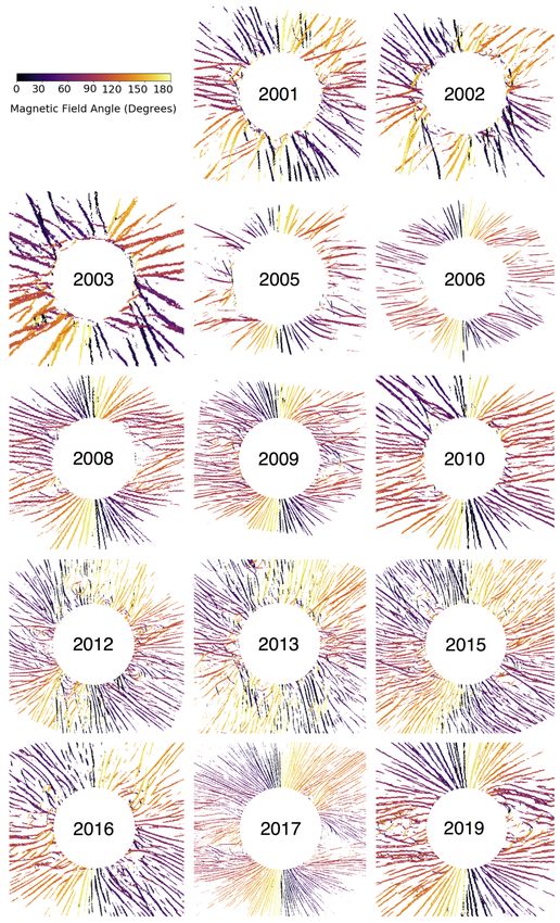
& Habbal 2007), but do not provide any information about the coronal magnetic field. The planned ASPIICS
coronagraph on PROBA-3 (Galano et al., 2018) intends to observe the continuum corona between ≈ 1.1 and 3
R , while METIS/COR on Solar Orbiter (Antonucci et al., 2017) will cover a variable distance range, where it can
observe between ≈ 1.2 to 3.0 R (1.6 to 4.1 R ) at minimum (maximum) orbital distance. ASPIICS and METIS
should provide images of the continuum coronal emission with substantially higher resolution, lower noise and less
scattered light compared to LASCO and STEREO, but will not surpass the radial extent and spatial resolution that
is possible to achieve during a TSE.
    Inferences of the coronal magnetic field topology are possible with Extreme Ultra-Violet (EUV) observations (e.g.
SDO/AIA; Lemen et al. 2012) as demonstrated by Schad 2017. However, they remain limited in spatial extent due
to their collisionally excited nature (see Section 1 of Boe et al. 2020 for an in-depth discussion). SWAP on PROBA-2
can perform slightly better, sometimes detecting EUV emission (Fe x 17.4 nm) as far as 2 R (Seaton et al., 2013),
but only in regions with a relatively high electron density (ne ). METIS promises to do even better, possibly reaching
3 R or more for the He ii 30.4 nm and H i 121.6 nm lines (Antonucci et al., 2017). Even with the improvements in
EUV observations, their collisionally excited nature (∝ n2e ) will cause them to be strongly weighted toward seeing
regions with higher electron density. Observing the corona in the EUV is consequently useful for studying the
magnetic loops above active regions and other structures in the low-corona (. 1.5 R ), but is not capable of fully
revealing the magnetic field line structure for the entire corona. At present, only during a TSE is the entire corona
– and its magnetic field structure – observable simultaneously from just above the photosphere out to at least 6 R .
    The first attempts to model the coronal magnetic field were based on extrapolations of the photospheric magnetic
field outward to an upper boundary, known as the ‘source surface’, beyond which the coronal magnetic field was
assumed to be radial. Originally proposed by Altschuler & Newkirk (1969) and Schatten et al. (1969), these so-called
Potential Field Source Surface (PFSS) models continue to evolve. The source surface has traditionally been set at
2.5 R from the Sun, but some more recent models have set the source surface as low as 1.5 R (Asvestari et al.,
2019) to attempt to best fit the open flux from coronal holes in the solar wind. More sophisticated models, such as
Magnetohydrodynamic (MHD) models (Mikić, 1990; Mikić et al., 1999), have been developed in an attempt to more
completely encompass the physics of the magnetized coronal plasma, but are more computationally expensive than
PFSS models.
    The photospheric magnetic observations used as the initial conditions for coronal models, such as those by the
Michelson Doppler Imager (MDI) on SOHO (Scherrer et al., 1995) and Helioseismic and Magnetic Imager (HMI) on
SDO (Scherrer et al., 2012), rely on line of sight Zeeman polarization effects. These observations are highly uncertain
for position angles greater than ≈ 45 to 75◦ from disk center (e.g. Altschuler & Newkirk 1969; Wiegelmann et al.
2017). Synoptic maps can compensate for this angle effect with solar longitude, provided the observations from an
entire solar rotation are combined. However, this process assumes that the coronal magnetic field does not change
substantially over a ≈ 28 day rotation period. Furthermore, observations of photospheric magnetic fields at the
poles have never been possible given that every solar magnetic field observatory is located near the ecliptic plane.
Even Ulysses (McComas et al., 1998), which reached a heliocentric latitude as high as ≈ 80◦ , did not have any
remote sensing instruments (magnetic measurements in situ only yield the in situ field strength and direction).
Solar Orbiter’s PHI (Solanki et al., 2015) promises to observe the polar photospheric field for the first time enabled
by its inclined orbit, though it will only be able to see one pole at a time for a subset of its orbit.
    PFSS, MHD and other models are powerful ways to explore the magnetic field of the corona and the origin of
the solar wind (see Wiegelmann et al. 2017 for a coronal modeling review), but to date these approaches have been
largely unconstrained due to the absence of magnetic field measurements in the corona. Even the most complex
MHD models, including a combination of coronal heating processes, are not capable of perfectly recreating the shape
of the solar corona when compared with TSE observations (Mikić et al., 2018). Furthermore, no model has been
quantitatively compared to the eclipse observations beyond a discussion of the general location and size of streamers
and coronal holes.
    In this work, we quantify the topology of the coronal magnetic field using TSE observations spread over almost
two complete solar activity cycles. We use an existing database of broadband white-light eclipse images (see Section
2), and apply the Rolling Hough Transform (developed by Clark et al. (2014), see Section 3) to automatically trace
the coronal magnetic field line structure. A detailed accounting of the observed features of the coronal magnetic
field are given in Section 4. Implications for coronal magnetic field, existing models and solar wind formation are
discussed in Section 5. Concluding remarks are given in Section 6.

                                                          2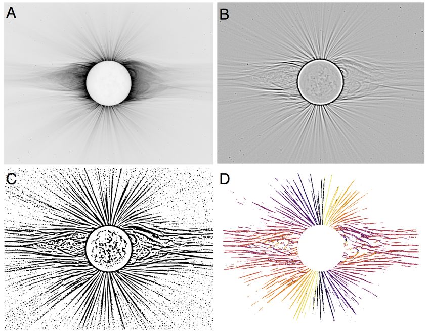
2          Data
Quantifying the structure of the magnetic field in the mid-corona (1.5 to 3 R ) has remained somewhat elusive
despite the advancement of ground- and space-based observatories (see Section 1), yet observing this region is crucial
for understanding the origins of the solar wind. The easiest way to simultaneously observe the entire corona (from
1 to at least 6 R ) with high spatial resolution and strong signal continues to be during a TSE. The many years of
existing TSE observations thus present a unique opportunity to quantify the magnetic field topology of the corona
throughout the solar cycle, and provide improved constraints for coronal modeling. We processed archival broadband
white-light total solar eclipse images taken between 2001 to 2019 to infer the magnetic field angle relative to the
radial direction for all solar latitudes (see Sections 3 and 4). These 14 eclipses span almost two complete solar cycles
and offer a unique probe of the direction of the coronal magnetic field.
    The entirety of the data used here was taken from an open source database of processed eclipse images 1 , which
comes from a variety of eclipse observers – both professionals and amateurs (see Table 2). All eclipse data were
stacked using the technique described in Druckmüller (2009), and processed with the Adaptive Circular High-pass
Filter (ACHF) method (Druckmüller et al., 2006) to enhance the magnetic field structure in the corona. Examples
of the white light coronal data from each of the 14 TSEs are shown in Figure 1. Note that the data are not
photometrically calibrated, so the intensity in the image is not representative of the relative intensity of the corona
between eclipses. The processing also changes the brightness contrast between different heliocentric distances. Several
of the white light images have been previously used to study individual eclipses (e.g. Habbal et al. 2010, 2014; Alzate
et al. 2017; Boe et al. 2018, 2020). For most eclipses, multiple cameras observed the corona at different angular
scales. The panels in Figure 1 show each of the coronae below 2.5 R . Examples from the much wider field images
(inside 5 R ), albeit with lower resolution, are shown in Figure 2.

             Date               Observing Location            Observers
             21 Jun 2001        Angola                        Úpice Observatory (Film camera)
             4 Dec 2002         South Africa                  Vojtech Rušin (Film camera)
             23 Nov 2003        Plane over Antartica          David Finlay
             4 Aug 2005         Ship in Pacific Ocean         Fred Espenak
             29 Mar 2006        Libya                         Peter Aniol, Massimiliano Lattanzi, Miloslav
                                                              Druckmüller, Hana Druckmüllerová
             1 Aug 2008         Mongolia                      Peter Aniol, Miloslav Druckmüller, Jan Sládeček,
                                                              Vojtech Rušin, Martin Dietzel
             22 Jul 2009        Marshall Islands              Peter Aniol, Miloslav Druckmüller, Vojtech Rušin,
                                                              L’ubomı́r Klocok, Karel Martišek, Martin Dietzel
             11 Jul 2010        Tatakoto                      Shadia Habbal, Martin Dietzel, Vojtech Rušin
             13 Nov 2012        Australia                     David Finlay, Constantinos Emmanouilidis, Man-To
                                                              Hui, Robert Slobins
             3 Nov 2013         Gabon                         Constantinos Emmanoulidis
             20 Mar 2015        Norway                        Shadia Habbal, Peter Aniol, Miloslav Druckmüller,
                                                              Pavel Štarha
             9 Mar 2016         Indonesia                     Don Sabers, Ron Royer
             21 Aug 2017        USA                           Shadia Habbal, Peter Aniol, Miloslav Druckmüller,
                                                              Zuzana Druckmüllerová, Jana Hoderovǎ, Petr
                                                              Štarha
             2 Jul 2019         Chile                         Peter Aniol, Miloslav Druckmüller

                    Table 1: Observing dates, locations and observers for the TSE data used in this work.

    1 a.   http://www.zam.fme.vutbr.cz/~druck/Eclipse/index.htm

                                                                  3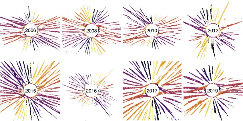
Figure 1: Inverted broadband white-light images of the solar corona during total solar eclipses that were processed
with the ACHF algorithm (see Section 2). The eclipse coronae are shown in chronological order from 2001 until
2019, cropped inside a 2.5 R square box. Solar north is oriented directly upward for all images. Note that these
images are not photometrically calibrated, so the brightness of the image cannot be compared between eclipses.

                                                        4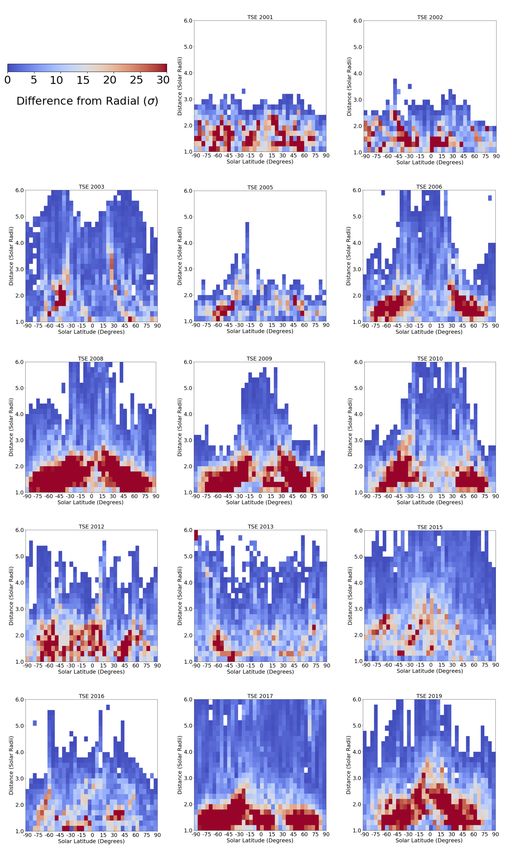
Figure 2: Inverted wide field broadband white-light images of the solar corona during total solar eclipses that were
processed with the ACHF algorithm (see Section 2). The eclipse coronae are shown in chronological order from 2006
until 2019, cropped inside a 5 R square box. Solar north is oriented directly upward for all images. Note that these
images are not photometrically calibrated, so the brightness of the image cannot be compared between eclipses.

3    RHT Field Line Tracing Method
Imbedded in this TSE dataset is a record of the coronal magnetic field topology with high spatial resolution between
1 and over 6 R , which is quantified here for the first time. It is important to underscore that the corona is
a 3-dimensional source; all the TSE images are line-of-sight (LOS) integrations of the corona, resulting in a 2D
image that has been collapsed into the plane-of-sky (POS). Since the coronal density drops sharply with heliocentric
distance, the observed intensity of the corona is substantially weighted toward the field lines that are the closest to
the solar limbs in the POS (perhaps ≈ ±20◦ of the POS). Thus, the final observables presented in this paper should
be considered as a density and angle weighted average of the coronal magnetic field in the vicinity of the POS.
    To quantify the coronal magnetic field structure, we apply a line tracing algorithm developed by Clark et al.
(2014) called the Rolling Hough Transform (RHT). The RHT algorithm was originally used to trace the magnetic
field of the Milky Way galaxy, and has been demonstrated with solar EUV data (Schad, 2017). Specifically, Schad
(2017) performed tests with the RHT algorithm indicating that it was a robust technique for detecting magnetic
field line edges – even with low signal to noise ratio data. The implementation of the RHT algorithm to the eclipse
dataset is based on that described by Schad (2017).
    First, the white light eclipse images are processed with a Gaussian high-pass filter, and then blurred at the same
resolution to enhance edges in the image and eliminate any low frequency structure that is not a direct result of the
magnetic field topology. Next the image is converted to a binary scale before finally being processed with the RHT
algorithm. An example of the procedure for an image from the 2019 TSE is shown in Figure 3. The RHT algorithm
determines the angle of the magnetic field line independently for each pixel with respect to the image coordinates (as
shown in Figs. 3, 4, 5 and 6, see Fig. 4 for the color scaling), by attempting to fit a line to every possible direction
inside a box centered on each pixel in the binary data. It then reports the relative probability for every possible field
angle direction, which is used to determine the uncertainty of each measurement, and the relative certainty between
various pixels. This process is repeated independently throughout the image, so every pixel in the final image is
a unique observation. The RHT algorithm does not connect features between pixels, so the lines seen in Figures
3, 4, 5 and 6 are not connected by the algorithm. Instead, the prevailing direction of the line is the same for the
collection of pixels along the line, and thus the continuity of the features (i.e. consistent angle/color) indicates that
the measurements are robust.

                                                           5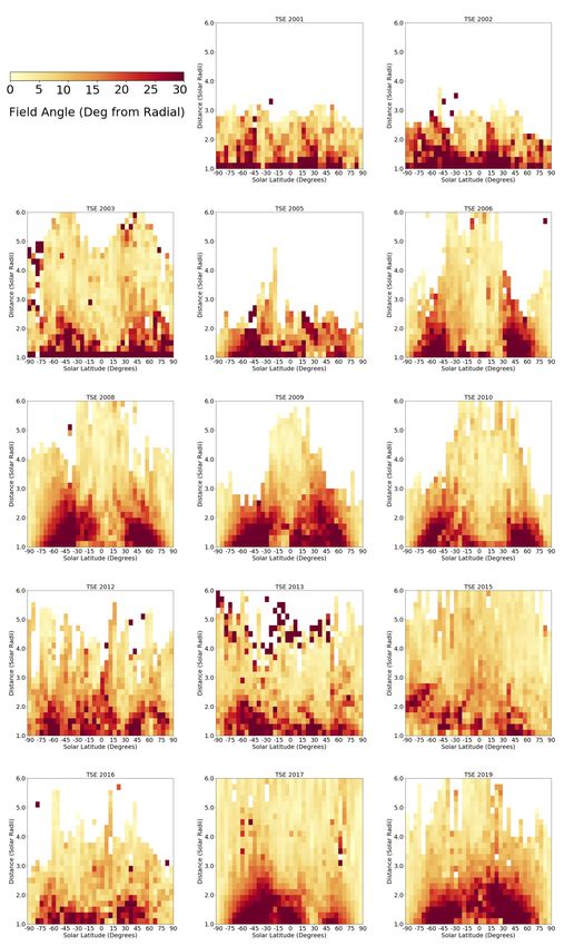
Figure 3: Example of the RHT procedure using the 2019 TSE corona. The inverted ACHF processed broadband
white light image (A), is filtered with a high-pass filter then blurred (B), then converted into a binary image (C).
Finally the binary image is fed through the RHT algorithm to measure the angle independently for each pixel (D),
with the color scaling shown in Figure 4.

    Since the TSE data were acquired with a wide range of telescopes and detectors of varying quality (2001 and
2002 were done with film), each eclipse had to be manually processed to maximize the field line structure in the
binary image. The Gaussian sigma of the high-pass filter ranged between σR = 0.002 and 0.05 R (in pixel units),
the RHT window size ranged from WRHT = 0.08 to 1.0 R , and the RHT smearing radius ranged between RRHT =
0.02 and 0.4 R (see Clark et al. (2014) and Schad (2017) for a discussion of these parameters and how they affect
the final results). In general, the final measured angle by the RHT algorithm is insensitive to the exact choice of
parameters (i.e. σR , WRHT and RRHT ). The main need for different parameters between eclipses is to maximize the
resolution, while still capturing the coronal field topology to as large a distance as possible. The only problems occur
when the structures are over-sampled or under-sampled. Over-sampling occurs where the size of the RHT fitting
box is smaller than the width of the field line in the binary image – causing the RHT algorithm to report angles
perpendicular to the true field line angle. Under-sampling occurs when the RHT fitting box is too large; in that case
it sees several different field lines at the same time, and thus is not capable of resolving the field line structure. These
effects necessitated changing the parameters manually to maximize the potential for the RHT algorithm to measure
the field line angles in the largest parameter space possible.

                                                             6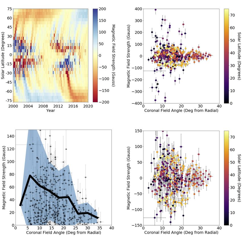
Figure 4: RHT measured field angle for the same eclipse images as shown in Figure 1. At each pixel, the RHT
algorithm reports a best fit angle with respect to the image frame. The color of the final points indicates the
measured angle. The same color scaling is used for all panels, as defined in the color bar at the top left.

    The initial angles returned by the RHT algorithm are given with respect to the image frame (as shown in Figs. 3,
4, 5 and 6). These angles are subsequently converted to be with respect to the radial direction. The angles relative
to radial prevent any angle discontinuity effects (i.e. 0◦ vs. 180◦ ) and enables a direct comparison of structures
throughout the corona for a single eclipse and between eclipses. In many cases, both narrow-field (typically 1-3 R )

                                                         7
Figure 5: RHT measured field angles for the wide field eclipse images shown in Figure 2. The exact same color
scaling is used as in Figure 4
and wide-field (often up to ≥ 6 R ) coronal data are available from the same eclipse. In a few cases, there were very
high resolution data of the lowest regions in the corona, which show detailed structures ubiquitously (see Figure 6).
When multiple images are available from a single eclipse, the data are stacked to generate a continuous measurement
from the lunar limb to several solar radii. All RHT data from the wide-field images below 2 R were removed from
the stacked results, due to the poor spatial resolution compared to the narrow-field images.
4 Results
The combined data from each eclipse are shown in Figure 7 as histograms of the field line angle with respect to the
radial direction. Figure 8 shows the same results as Figure 7, but in units of the relative uncertainty for the given bin
(i.e. the statistical significance of the difference from radial). The uncertainties are propagated through the weighted
mean inside each bin based on the reported RHT probabilities for each data point inside the bin.
The direction of the coronal magnetic field with respect to the radial direction, for the individual eclipses shown
in Figures 7 and 8, indicates a high variance in coronal structures over the solar cycle. Near solar minimum (roughly
2009 and 2019), the corona has two lobes of highly non-radial field lines between about 15 and 75◦ latitude in the
North and South. The location of the non-radial lobe tends to move toward the equator with higher heliocentric
distance, ending around 2.5 to 3 R . Near solar maximum (roughly 2001 and 2013), small pockets of non-radial
field topology appear throughout the corona without the large-scale lobe structure as seen at solar minimum. These
observations are consistent with the concept that the coronal magnetic field is dominated by dipolar and quadrupolar
magnetic moments during solar minimum, while higher order moments begin to have a larger impact on the global
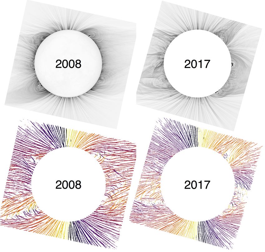
coronal magnetic field at solar maximum. Indeed, the shape of the coronal magnetic field topology is strikingly
similar for the eclipses near solar minimum, which is especially noticeable in the highest resolution TSE data (from
2008 and 2017) shown in Figure 6.
Averaging the individual eclipse data every two years across all position angles (Figure 9) shows the global
divergence of the coronal magnetic field angle from the radial direction with the expansion of the solar wind. There
does not appear to be an obvious solar cycle dependence in the average radial angle (for the entire corona), except
for a slightly more non-radial angle during solar minimum in 2009 and 2019. It is clear from Figures 7, 8 and 9,
that the corona is consistently non-radial (≥ 10◦ ) out to 3 R or more, to a high confidence level. The distance at
which the coronal field becomes statistically consistent with radial does move slightly outward for the more recent
eclipses, but this effect is due to the increased spatial resolution of the recent eclipse observations that allow for more
8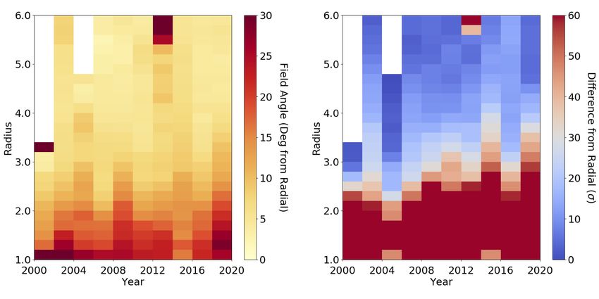
Figure 6: Example of the two highest resolution coronal images that were used in this study. The top panels show
the original inverted eclipse images, with the corresponding RHT measurement below. The same scaling is used
on the RHT angle colors as in Figure 4. Fine-scale structure is visible ubiquitously throughout the corona, with
topologically ‘open’ field lines dominating the majority of the corona, even at 1.2 R .

independent measurements of the coronal magnetic field inside the same bin (thus decreasing the uncertainty). At
a distance of about 4 R however, the field does become almost entirely radial. One notable exception is the highly
non-radial structure at 6 R in 2013, which is due to a Coronal Mass Ejection (CME) that was previously reported
by Alzate et al. (2017).
    The average deviation of the magnetic field from radial at different coronal latitudes over the past 20 years of
observations is shown in Figure 10, where the field angle measurements between 1.5 and 3.0 R are averaged for all
eclipse data in two year periods. During solar minimum there are large, highly non-radial regions between 15 and 75◦
latitude, both in the north and south. While the mid-latitudes have a highly non-radial field during solar minimum,
the field lines above the poles are almost precisely radial. During solar maximum, there are more non-radial fields
throughout the entire corona, but the difference from radial is substantially smaller than in the solar minimum lobes

                                                         9
Figure 7: Magnetic field angle with respect to radial for all eclipses used in this work. The RHT data is stacked (for
TSEs with multiple images available) and binned to create the final result shown here (See Section 3 for details).
at mid-latitudes. Throughout the solar cycle, there exist mostly radial fields above the solar equator.
The coronal magnetic field topology is compared with the photospheric magnetic field in Figure 11. The photo-
spheric magnetic field data in the top left panel of Fig 11 are a compilation of SOHO/MDI (Scherrer et al., 1995) and
SDO/HMI (Scherrer et al., 2012) photospheric magnetic field observations. Level 2 synoptic maps were averaged in
magnetic field strength at all longitudes for each Carrington rotation. For epochs where both MDI and HMI were
10Figure 8: Statistical significance of how far the magnetic field was from the radial direction, based on the data in
Figure 7 divided by the uncertainty of the mean field angle measurement in each bin.
operational, we averaged the two datasets. We then compared the photospheric magnetic field strength with the
average magnetic field angle observed in the corona above, between 1.5 and 3.0 R . Every latitude bin for each
eclipse (as in Figs. 7 and 8) is compared to the same latitude in the photospheric magnetic field for the Carrington
rotation of the given eclipse. The scatter of the correlation between the photospheric field strength and the coronal
field angle is shown with different scalings in the remaining panels of Figure 11. The top right and bottom right
11Figure 9: Average magnetic field angle with respect to radial (left), and the statistical significance that the measured
angle is non-radial (right), at different heliocentric distances. The TSE data is averaged over all position angles and
all eclipses available for every two year period between 2000 and 2020.
Figure 10: Average magnetic field angle with respect to radial (left), and the statistical significance that the measured
angle is non-radial (right) at different solar latitudes. The TSE data is averaged over a distance range of 1.5 to 3.0
R and all eclipses available for every two year period between 2000 and 2020.
panels are identical except for the scaling of the magnetic field strength to show different structures in the data (see
Section 5). The bottom left panel shows the average magnetic field strength (absolute value) for different coronal
field angles. The regions of the highest magnetic field curvature (& 20 degrees from radial) all have a weak average
magnetic field below in the photosphere, while the regions of the highest magnetic field strength in the photosphere
tend to result in a much more radial coronal magnetic field.
12Figure 11: Top left: Compilation of SOHO/MDI and SDO/HMI synoptic map magnetic field measurements averaged
over all solar longitudes for each Carrington rotation, within every 5 degrees of solar latitude between -75 and 75.
Top right: Average magnetic field strength in the photosphere at the same Carrington rotation at the time of each
TSE, compared to the average field angle in the corona between 1.5 and 3.0 R . The color of the points indicates
the absolute value of the solar latitude for the data. Bottom left: Same as top right, but with the absolute value
of magnetic field strength. The black line indicates the mean field strength for every 4 degrees of deviation from a
radial magnetic field, and the blue region indicates the 1 σ spread on the mean. Bottom right: Same as top right,
but with decreased bounds on the magnetic field strength (|B| < 150 G) to show detail in the distribution.
135 Discussion
As described in Section 4, the RHT algorithm is used here to infer the coronal magnetic field topology for 14 unique
eclipse coronae – covering two solar activity cycles. These results establish that the coronal magnetic field is almost
always non-radial below 4 R , and that the distribution of the non-radial fields is a function of latitude and solar
cycle. Next, we give an overview of the inferred topology for the coronal magnetic field and discuss the implications
of these results for coronal models and solar wind formation.
5.1 Fine-scale Structure and Coronal Radiality
In all the TSE magnetic field inferences, very fine-scale structure is present and appears limited only by the spatial
resolution of the observations. The higher resolution TSE data from the past few years show increasingly fine-scale
magnetic field structure, as illustrated by the two cases presented in Figure 6. Coronagraphs have been used to
previously explore the fine-scale structure of the corona, especially with regard to observing the evolution of CMEs
from the corona into the heliosphere (e.g. Gopalswamy et al. 2009). DeForest et al. (2018) previously demonstrated
not only the presence of fine-scale structures in the outer corona (& 3 R ), but also their dynamical evolution on
short time scales. These observations are only possible with current coronagraphs when using exceptionally long
exposure times combined with modern image processing techniques. The eclipse data presented here indicate that
the fine-scale structures are present from the outer corona region explored by DeForest et al. (2018), through the
mid-corona (1.5 to 3 R ) and down to the solar surface.
Missing from current coronagraph data however, is information about the mid-corona between about 1.5 and 3
R (see Section 1). Insights into this data gap are provided at present by TSE observations as done here. In general,
we find that the coronal magnetic field is non-radial in the low corona (. 1.5 R ) and becomes increasingly radial
at higher heliocentric distances – typically becoming entirely radial around 4 R . The coronal field is the most
non-radial during solar minimum, where lobes of curved fields (≈ 15◦ up to 60◦ from radial) exist between about 15
and 75◦ latitude (see Figs. 7, 8 and 10). The lobes are often tipped toward the equator, where the higher latitude
regions become increasingly radial at lower heliocentric distances. These lobes often have a gap of almost radial
field lines between them near the equator, which perhaps can be thought of as the signature of the beginning of the
heliospheric current sheet. Likely the shape and presence of this morphology during solar minimum indicates that
the corona is dominated by a dipolar and quadrupolar field component. During solar maximum, the corona is less
organized; small scale non-radial structures are ubiquitous, they vary wildly between eclipses and do not extend to
nearly as large of a heliocentric distance.
Comparing the photospheric magnetic field with the average magnetic field angle in the middle corona (see Fig.
11) suggests that, on average, strong photospheric fields (|B| & 100 G , see Section 4) result in more radial fields in
the corona above. Clearly there are closed field lines in the lower corona around strong field regions with sunspots
and filaments/prominences, but they typically do not appear to extend into the mid-corona. There can be radial
fields above weak regions, but stronger photospheric fields are correlated with a more radial coronal field.
5.2 Implications for PFSS and MHD Models
Potential Field Source Surface (PFSS) models have long been used as a simple way to model the coronal magnetic
field, using the photospheric magnetic field as a boundary condition (see Section 1). Implicit in the model is an
assumption of a source surface radius, beyond which the field is assumed to be entirely radial. The source surface
is often set at 2.5 R , but has been set as low as 1.5 R (e.g. Asvestari et al. 2019). Our inferences of the coronal
magnetic field topology clearly indicate that this is not a valid assumption for any period throughout the solar cycle.
In fact, Figures 7, 8, and 9 indicate that the coronal magnetic field is non-radial often out to 3 R , with some
eclipses having regions of the corona that remain non-radial to beyond 4 R . The topology of the magnetic field in
the middle corona (see Fig. 10) establishes that the deviation from the radial direction depends strongly on latitude
and solar cycle. Clearly the distance at which the coronal field becomes radial is a constantly fluctuating and complex
boundary between about 2 and 4 R around the Sun. This radial distance follows a behavior similar to the shape
of the freeze-in distances of Fe 10+ and Fe 13+ as observed with 2015 TSE data by Boe et al. (2018), where the ions
had lower freeze-in distances in coronal holes, compared to the streamers. This work provides the first observational
evidence in support of a non-spherical source surface, as suggested by Riley et al. (2006) using MHD modeling.
14The main, and currently unavoidable, limitation of PFSS and MHD models is the necessity of photospheric
magnetic field observations, which are restricted to around 75 degrees latitude of the equator – and the need for a
full rotation of data to probe all solar longitudes (this may be improved soon with Solar Orbiter, see Section 1).
Still, the most complex 3D MHD models coupled with coronal heating models (i.e. Mikić et al. 2018) are able to
generate a somewhat reasonable field line structure for the middle corona, especially if the polar flux is corrected in
the model to qualitatively fit a TSE image as shown by Riley et al. (2019). Indeed, the choice of model parameters
can strongly influence the state of the modeled plasma as well as the magnetic field topology (Lionello et al., 2009;
Downs et al., 2010). The more traditional and lower resolution PFSS models (e.g. see Wiegelmann et al. 2017) with
low source surfaces (≤ 2.5 R ) however, appear to over predict the curvature of the coronal magnetic field compared
to what we have inferred in this work. It is not clear if this is an issue with insufficient model resolution, an improper
selection of the source surface, or perhaps both.
Under-resolved structures and incorrect assumptions about the coronal magnetic field will have impacts on models
of the extended corona and beyond, as PFSS and MHD models are commonly used as a tool to link solar wind observed
in situ back to specific sources on the Sun (e.g. Zhao et al. 2017). The magnetic field angle results presented here
could be used as a constraint for future PFSS and MHD models, in combination with the photospheric field, especially
to nail down the somewhat elusive high-latitude magnetic field strength (as explored by Riley et al. 2019).
5.3 Implications for Solar Wind Formation
Even though the typical angle of magnetic field lines in the low corona is non-radial, many of the fine-scale structures
present throughout the eclipse coronae presented in this work (see Section 5.1) can be traced continuously from just
above the lunar limb outward to several solar radii (see Fig. 5). Once a field line appears almost radial at more
than ≈ 3 or 4 R , it is probably safe to assume that the field line is open and the plasma on that field line will flow
the heliosphere to create solar wind. Given that the rays seen at ≈ 3 − 6 R connect to structures at almost every
latitude back to the solar limb, this suggests that a large fraction of the field lines emerging from the low corona are
in fact open field lines. Of course, we cannot concretely conclude that these lines are indeed open flux without a
direct measurement of the magnetic field, but the inferred magnetic topology presented here seems to imply that this
is the case. Such apparently ‘open’ field lines are present seemingly regardless of the presence or absence of coronal
holes on the solar disk. Occasionally, these ‘open’ field line structures are projected into the same line of sight as
closed field regions, indicating that the closed field region does not dominate the entire line of sight.
The idea that open flux may indeed be originating from what might be classically considered as a ‘closed’ structure
(e.g. an active region) has been suggested previously by Sakao et al. (2007) and Harra et al. (2008) using soft X-ray
observations. Additionally, EUV spectroscopy with EIS on Hinode has found Doppler-shifted outflows of 20-50 km
s− 1 that can persist for dozens of hours above an active region (Doschek et al., 2008). Recent work with high
resolution PFSS models have shown that open flux can be rooted in and near active regions and streamers (e.g.
DeRosa & Barnes 2018), and that the outflows at low latitude regions (< 40 degrees) can explain the mass loss
needed to create the slow solar wind (Brooks et al., 2015). Even the fast solar wind flux cannot be fully accounted
by coronal holes alone (Linker et al., 2017)
Recently, some studies have focused on the interaction of coronal holes adjacent to streamers and active regions
(open-closed boundary) as a mechanism to explain the slow solar wind (e.g. Antiochos et al. 2011; Titov et al. 2011).
These models seem to account somewhat for the complexity of the solar wind, and the presence of open flux near
the solar equator, but still appear to overestimate the field line curvature (see Section 5.2) and underestimate the
fine-scale structure seen in the TSE corona (see Section 5.1) – likely due to an insufficient model resolution. Perhaps
an explicit coronal hole, or coronal hole boundary, is not required to explain the diversity of solar wind plasma
characteristics. Instead, there could be regions of the quiet Sun which can in fact inject plasma into the solar wind
(e.g. Linker et al. 2017; Riley et al. 2019). If that is the case, then the precise speed and composition of the solar
wind in situ can be explained simply by the different thermodynamical properties of different regions in the low
corona (Habbal & Woo, 2001; Xu & Borovsky, 2015).
6 Conclusions
Application of the Rolling Hough Transform (RHT) to white-light TSE images, as done here for 14 eclipses between
2001 and 2019, has demonstrated that TSE observations continue to yield unique opportunities to quantify the
15topology of the coronal magnetic field throughout the solar cycle – thus providing valuable constraints for coronal
modeling and solar wind formation. In particular, this work showed that:
1. The coronal magnetic field is highly structured down to the spatial resolution of the images, with topologically
‘open’ field line structures visible at most latitudes throughout the corona for all solar eclipse images.
2. The coronal field can evolve significantly in the mid-corona (1.5 to 3 R ) between different latitude regions
over the solar cycle, often remaining non-radial out to about 4 R .
3. The most non-radial regions in the mid-corona occur above the weakest photospheric magnetic fields, whereas
regions with the strongest fields are correlated with nearly radial field lines.
4. These TSE observations yield essential constraints for coronal models. We find that the canonical source surface
of 2.5 R in PFSS models is not far enough from the Sun, and that the source surface is non-spherical.
The RHT algorithm and procedure presented here could be used in the future with coronagraphic observations,
especially with the upcoming METIS and ASPIICS coronagraphs. Inferring the coronal magnetic field topology
may consequently be possible for a much larger and almost continuous dataset. The RHT tracing method could
be useful for mapping the structures of CMEs in the corona and as a tool to empirically link in situ solar wind
observations to sources on the Sun, without any assumptions whatsoever on the origin of the structure from just
above the photosphere to at least the source surface region.
Acknowledgments
This work would not have been possible without the many years of hard work and dedication of all the eclipse
observers, given in Table 2. Special thanks to Xudong Sun for suggesting the RHT algorithm for use with eclipse
data. We thank the reviewer for their exceptionally fair and insightful comments. Financial support was provided
to B. Boe by AURA/NSO with grant N97991C to the Institute for Astronomy at the University of Hawaii. NASA
grant NNX17AH69G and NSF grants AGS-1358239, AGS-1255894, and AST-1733542 to the Institute for Astronomy
of the University of Hawaii. M. Druckmüller was supported by the Grant Agency of Brno University of Technology,
project No. FSI-S-20-6187.
References
Altschuler, M. D., & Newkirk, G. 1969, Sol. Phys., 9, 131
Alzate, N., Habbal, S. R., Druckmüller, M., Emmanouilidis, C., & Morgan, H. 2017, ApJ, 848, 84
Antiochos, S. K., Mikić, Z., Titov, V. S., Lionello, R., & Linker, J. A. 2011, ApJ, 731, 112
Antonucci, E., Andretta, V., Cesare, S., et al. 2017, in Society of Photo-Optical Instrumentation Engineers (SPIE)
Conference Series, Vol. 10566, Proc. SPIE, 105660L
Asvestari, E., Heinemann, S. G., Temmer, M., et al. 2019, Journal of Geophysical Research (Space Physics), 124,
8280
Boe, B., Habbal, S., Druckmüller, M., et al. 2020, ApJ, 888, 100
—. 2018, ApJ, 859, 155
Brooks, D. H., Ugarte-Urra, I., & Warren, H. P. 2015, Nature Communications, 6, 5947
Brueckner, G. E., Howard, R. A., Koomen, M. J., et al. 1995, Sol. Phys., 162, 357
Clark, S. E., Peek, J. E. G., & Putman, M. E. 2014, ApJ, 789, 82
Darwin, L., Schuster, A., & Maunder, E. W. 1889, Philosophical Transactions of the Royal Society of London Series
A, 180, 291
16DeForest, C. E., Howard, R. A., Velli, M., Viall, N., & Vourlidas, A. 2018, ApJ, 862, 18
DeRosa, M. L., & Barnes, G. 2018, ApJ, 861, 131
Dima, G. I., Kuhn, J. R., & Schad, T. A. 2019, ApJ, 877, 144
Doschek, G. A., Warren, H. P., Mariska, J. T., et al. 2008, ApJ, 686, 1362
Downs, C., Roussev, I. I., van der Holst, B., et al. 2010, ApJ, 712, 1219
Druckmüller, M. 2009, ApJ, 706, 1605
Druckmüller, M., Rušin, V., & Minarovjech, M. 2006, Contributions of the Astronomical Observatory Skalnate Pleso,
36, 131
Galano, D., Bemporad, A., Buckley, S., et al. 2018, in Society of Photo-Optical Instrumentation Engineers (SPIE)
Conference Series, Vol. 10698, Proc. SPIE, 106982Y
Gibson, S. E., Dalmasse, K., Rachmeler, L. A., et al. 2017, ApJ, 840, L13
Gopalswamy, N., Yashiro, S., Michalek, G., et al. 2009, Earth Moon and Planets, 104, 295
Habbal, S. R., Morgan, H., & Druckmüller, M. 2014, ApJ, 793, 119
Habbal, S. R., Morgan, H., Druckmüller, M., & Ding, A. 2010, ApJ, 711, L75
Habbal, S. R., & Woo, R. 2001, ApJ, 549, L253
Habbal, S. R., Woo, R., & Arnaud, J. 2001, ApJ, 558, 852
Hale, G. E., Ellerman, F., Nicholson, S. B., & Joy, A. H. 1919, ApJ, 49, 153
Harra, L. K., Sakao, T., Mandrini, C. H., et al. 2008, ApJ, 676, L147
Kaiser, M. L., Kucera, T. A., Davila, J. M., et al. 2008, Space Sci. Rev., 136, 5
Lemen, J. R., Title, A. M., Akin, D. J., et al. 2012, Sol. Phys., 275, 17
Linker, J. A., Caplan, R. M., Downs, C., et al. 2017, ApJ, 848, 70
Lionello, R., Linker, J. A., & Mikić, Z. 2009, ApJ, 690, 902
Maunder, E. W. 1899, The Indian eclipse, 1898 : report of the expeditions organized by the British Astronomical
Association to observe the total solar eclipse of 1898 January 22
McComas, D. J., Bame, S. J., Barraclough, B. L., et al. 1998, Geophys. Res. Lett., 25, 1
Mikić, , Z., Downs, C., et al. 2018, Nature Astronomy, 2, 913
Mikić, Z. 1990, Physics of Fluids B, 2, 1450
Mikić, Z., Linker, J. A., Schnack, D. D., Lionello, R., & Tarditi, A. 1999, Physics of Plasmas, 6, 2217
Morgan, H., & Habbal, S. R. 2007, A&A, 471, L47
Munro, R. H., & Withbroe, G. L. 1972, ApJ, 176, 511
Newkirk, Gordon, J. 1967, ARA&A, 5, 213
Riley, P., Linker, J. A., Mikic, Z., et al. 2019, ApJ, 884, 18
Riley, P., Linker, J. A., Mikić, Z., et al. 2006, ApJ, 653, 1510
Saito, K. 1958, PASJ, 10, 49
17Sakao, T., Kano, R., Narukage, N., et al. 2007, Science, 318, 1585
Schad, T. 2017, Sol. Phys., 292, 132
Schatten, K. H., Wilcox, J. M., & Ness, N. F. 1969, Sol. Phys., 6, 442
Scherrer, P. H., Bogart, R. S., Bush, R. I., et al. 1995, Sol. Phys., 162, 129
Scherrer, P. H., Schou, J., Bush, R. I., et al. 2012, Sol. Phys., 275, 207
Schwabe, H. 1844, Astronomische Nachrichten, 21, 233
Seaton, D. B., De Groof, A., Shearer, P., Berghmans, D., & Nicula, B. 2013, ApJ, 777, 72
Solanki, S. K., del Toro Iniesta, J. C., Woch, J., et al. 2015, in IAU Symposium, Vol. 305, Polarimetry, ed. K. N.
Nagendra, S. Bagnulo, R. Centeno, & M. Jesús Martı́nez González, 108–113
Titov, V. S., Mikić, Z., Linker, J. A., Lionello, R., & Antiochos, S. K. 2011, ApJ, 731, 111
van de Hulst, H. C. 1950, Bull. Astron. Inst. Netherlands, 11, 135
Van Vleck, J. H. 1925, Proceedings of the National Academy of Science, 11, 612
Wiegelmann, T., Petrie, G. J. D., & Riley, P. 2017, Space Sci. Rev., 210, 249
Woo, R., & Habbal, S. R. 1997, Geophys. Res. Lett., 24, 1159
Xu, F., & Borovsky, J. E. 2015, Journal of Geophysical Research (Space Physics), 120, 70
Zhao, L., Landi, E., Lepri, S. T., et al. 2017, ApJ, 846, 135
18You can also read