Throughput Prediction on 60 GHz Mobile Devices for High-Bandwidth, Latency-Sensitive Applications
←
→
Page content transcription
If your browser does not render page correctly, please read the page content below
Throughput Prediction on 60 GHz Mobile
 Devices for High-Bandwidth, Latency-Sensitive
                  Applications

    Shivang Aggarwal1 , Zhaoning Kong2 , Moinak Ghoshal1 , Y. Charlie Hu2 ,
                           Dimitrios Koutsonikolas1
              1
                  Northeastern University, USA 2 Purdue University, USA
       Abstract. In the near future, high quality VR and video streaming at
       4K/8K resolutions will require Gigabit throughput to maintain a high
       user quality of experience (QoE). IEEE 802.11ad, which standardizes
       the 14 GHz of unlicensed spectrum around 60 GHz, is a prime candidate
       to fulfil these demands wirelessly. To maintain QoE, applications need
       to adapt to the ever changing network conditions by performing quality
       adaptation. A key component of quality adaptation is throughput pre-
       diction. At 60 GHz, due to the much higher frequency, the throughput
       can vary sharply due to blockage and mobility. Hence, the problem of
       predicting throughput becomes quite challenging.
       In this paper, we perform an extensive measurement study of the pre-
       dictability of the network throughput of an 802.11ad WLAN in down-
       loading data to an 802.11ad-enabled mobile device under varying mobil-
       ity patterns and orientations of the mobile device. We show that, with
       carefully designed neural networks, we can predict the throughput of the
       60 GHz link with good accuracy at varying timescales, from 10 ms (suit-
       able for VR) up to 2 s (suitable for ABR streaming). We further identify
       the most important features that affect the neural network prediction
       accuracy to be past throughput and MCS.

1    Introduction
The past few years have witnessed the rise of a number of high-bandwidth,
latency-sensitive applications including virtual reality (VR), high-resolution
video streaming, live video streaming, and connected autonomous vehicles. Such
applications are characterized by stringent user-perceived quality of experience
(QoE) requirements, which in turn dictate high demand for the network per-
formance in terms of ultra high throughput and low latency. Further, such ap-
plications typically run on mobile devices, which require high network perfor-
mance to be supported wirelessly. For example, 8K resolution VR demands 1.2
Gbps [28] in order to satisfy the 20ms photon-to-motion latency, while live 4K
video streaming at 30 FPS demands 1.8 Gbps [16] for good user QoE.
    Such stringent demand for network performance could not be supported in
the past decade. However, the advent of mmWave technologies in recent years
has made such network performance within reach and holds the promise to
enable these demanding applications. For example, the IEEE 802.11ad WLAN
standard [20] governs the use of the unlicensed spectrum around 60 GHz and
supports 2 GHz wide channel to provide PHY data rates of up to 6.7 Gbps.
2
However, 60 GHz networks also come with higher dynamics due to their
vastly different propagation characteristics compared to sub-6 GHz networks. In
particular, due to the high attenuation loss at 60 GHz, directional communica-
tion is needed, making the wireless link highly susceptible to human blockage
and mobility [43,42]. Due to these challenges, a user watching a 360◦ video or
playing a VR game over a 60 GHz network may experience long periods of
rebuffering/stalls due to intervals of low to no connectivity [44,48,16]. For exam-
ple, the user may be moving around in such a way so as to face completely away
from the AP and thus self-block the link. For this reason, a 60 GHz WLAN often
cannot be used as a standalone technology to enable these high resolution ap-
plications, and the legacy sub-6 GHz WiFi, which does not suffer from blockage
and mobility, may be required as a backup [42,16].
Fortunately, most of the network-demanding applications already have some
type of quality adaptation built-in, to deal with the network dynamics. For ex-
ample, adaptive bitrate (ABR) streaming has become a de facto mechanism
implemented in modern video streaming systems such as YouTube, backed by a
number of adaptive streaming standards introduced over the years [40,33,3,11].
In a nutshell, ABR streaming continuously monitors the network conditions and
adapts the content quality to optimize the QoE, which typically is a function of
the frame resolution, frame continuity, and rebuffering time. ABR streaming has
been applied in all the recent proposals for high-resolution 360o video stream-
ing [34,18,37] as well as live video streaming [16]. Similar adaptation techniques
have also been proposed for state-of-the-art mobile VR systems [26].
The very first task of network adaptation in such network-demanding appli-
cations is the estimation of network conditions for the next time interval. For
example, in video streaming, most ABR systems estimate the throughput in the
next time interval and choose a video quality level based on the throughput es-
timate and playback buffer occupancy [41,39], as both can affect the QoE. More
recently, the use of deep learning (DL) to select the most appropriate quality
level has gained popularity [29,46] and ML-based ABR algorithms have been
shown to outperform traditional algorithms.
The unique characteristics of the 60 GHz links, however, make throughput
prediction in 60 GHz WLANs a much more challenging problem than in legacy
WLANs. Although throughput estimation/prediction has been studied in the
past in the context of sub-6 GHz WLANs [23,38,22] and cellular networks [27],
no previous work, to our best knowledge, has studied throughput prediction at
60 GHz networks. In this work, we carry out the first measurement study of the
throughput predictability in 60 GHz WLANs using ML.
There are two main challenges to conduct this measurement study. First,
in order to reliably train and test any ML model, we need to collect a signifi-
cant amount of data. Since 60 GHz WLANs are not widely deployed (the first
802.11ad-enabled smartphone model was only launched in 2019), we cannot col-
lect data from real networks, as in previous ABR studies [29,46]. Further, the only
two phones that support 802.11ad, the ASUS ROG Phone [5] and the ASUS ROG
Phone II [6], are not VR Ready; hence, we cannot perform real VR experiments3
with volunteers, as in previous VR studies [26,45]. Thus, we need to develop a
methodology to collect traces in a controlled environment efficiently and in an
automated way, in order to obtain a large amount of data while covering a wide
variety of realistic mobility patterns. To meet these conflicting requirements, we
mounted the 802.11ad phone on a programmable 3-axis motion controller typ-
ically used by professional photographers. Using this setup, we collected more
than 100 hours of traces while running different applications under random mo-
bility patterns. Second, unlike in previous works, which make predictions only
on coarse-grained timescales, e.g., in the order of a few seconds for ABR video
streaming [47,46], we study throughput prediction at timescales as fine as 10 ms,
which are needed by some of the demanding applications such as VR. To support
throughput prediction at such fine timescales, we need ML models that strike
a good balance between being accurate as well as being lightweight enough to
run on mobile devices within such short timescales. To overcome this challenge,
we started with a neural network model previously shown to work well at the
2-second timescale [46], and performed multiple iterations of grid search on the
two configuration dimensions (number of layers and number of nodes) to find
the smallest configuration, beyond which the performance increase is marginal,
to derive a model configuration that balances accuracy and inference latency.
We also considered a recurrent neural network (RNN) model, Long Short Term
Memory (LSTM), which is suitable for processing time series data, as is the case
with throughput prediction. We again went through configuration search to ar-
rive at a cost-effective LSTM model for our throughput prediction problem. We
then experimentally compared both models throughout our measurement study.
In summary, our work makes the following contributions.
– We conducted the first measurement study of the throughput predictability
of a 60 GHz WLAN to a mobile device. The dataset is publicly available [1].
– We tuned the parameters of state-of-the-art throughput-prediction DNNs to
strike a balance between prediction accuracy and lightweightness usable for
online throughput prediction. Our two models run in 0.41ms and 4.02 ms on
the ASUS ROG Phone II and require less than 4 MB of memory.
– We found that TCP throughput prediction in static scenarios is highly accu-
rate for 40 to 2000 ms, with 95th percentile error ranging between 10.6% for
40 ms and 5.7% for 2 s. For 10-20 ms, the accuracy drops but still remains
at satisfactory levels.
– However, the accuracy drops in random mobility scenarios, typical of real
applications. The 95th percentile error increases to 38.1% for 10 ms and
19.4% for 2 s timescales.
– We performed a feature selection study and found that only a few features are
important to make accurate throughput predictions. At timescales smaller
than 100ms, past throughput is the most important, but for larger timescales,
MCS becomes more useful.
– Our study suggests that VR apps should be conservative in the use of
throughput prediction. In particular, at the 10ms timescale the prediction
error is above 10% for 40% of the time, and the 95th percentile prediction
error is 38%.4
2 Experimental Methodology
Devices We used a Netgear Nighthawk X10 Smart WiFi router [12] and an
ASUS ROG Phone II [6] for our measurements. The Netgear router has a 10-
Gigabit SFP+ Ethernet port, which we use to connect to a powerful desktop
acting as the server in our experiments. The ASUS ROG Phone II has an octa-
core Snapdragon 855 Plus processor with a maximum CPU frequency of 2.96
GHz, a 6000 mAh battery, and an 8 GB RAM, and runs the Android OS 10.
Both devices support all 12 802.11ad single carrier MCSs, yielding theoretical
data rates up from 385 Mbps to 4.6 Gbps. However, similar to previous studies
using laptops as 802.11ad clients [35,16,36], the maximum TCP throughput is
limited to 1.65 Gbps in practical scenarios.
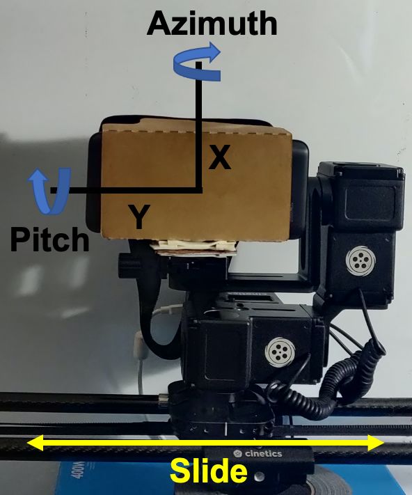
Experimental Setup and Trace Collection In all
our experiments, except for those with real applica-
tions in §3.4, we used nuttcp [13] with the default CU-
BIC congestion control to generate backlogged TCP traf-
fic from the server to the phone and logged through-
put every 10 ms. We developed an Android app that
runs on the phone and logs sensor and link state in-
formation. This information is used as input in the ML
models, described in §2. Specifically, the app uses the Fig. 1: Mobility Ex-
Android Sensor API [4] to log information from the periments Setup
TYPE ROTATION VECTOR/TYPE GAME ROTATION VECTOR sensors, which report the
phone’s rotation angle in the azimuth and pitch dimensions (Fig. 1), and from
the accelerometer (TYPE ACCELEROMETER) sensor, which gives the acceleration of
the phone (in m/s2 ) on the x-, y-, and z-axis. Sensor data are logged every 10
ms. The app also logs 60 GHz link information reported by the wil6210 driver
on the phone every 20 ms. This includes the MCS used by the AP for data trans-
mission, link quality estimators (SQI, RSSI), the link status (OK, RETRYING,
FAILED), and the selected beamforming sectors.
Since 60 GHz WLANs are not widely deployed, we cannot collect data from
real networks, as in previous ABR studies over the Internet [29,46]. In addi-
tion, our phone is not VR Ready and we cannot perform real VR experiments
with volunteers, as in previous VR studies [26,45]. Hence, we used the following
methodology to collect a large amount of data, while covering a wide variety of
realistic mobility patterns in a controlled environment efficiently and in an auto-
mated way. For all our experiments, we kept the phone in a Google Cardboard [9]
headset at a distance of 4 m from the AP, to emulate a realistic signal prop-
agation environment. For the experiments involving mobility, we mounted the
headset on a Cinetics Lynx 3-Axis Slider [7], used by professional photographers
(Fig. 1). This setup enabled us to perform full 360◦ rotation in the azimuth and
pitch dimensions at a speed of up to 48◦ /s and translational motion of up to 1
m. We used the Dragonframe software [8] to program custom mobility patterns
(e.g., emulating a user playing a VR game or watching a 360◦ video). Using this
methodology, we collected over 100 hours of traces.
Trace Processing Applications have diverse requirements on the timescale
of throughput prediction. For example, VR applications need to predict the5
throughput in the window of the next tens of milliseconds. On the other end of
the spectrum, video streaming applications usually fetch video chunks of several
seconds in length and therefore need to predict the average throughput in the
window of the next few seconds. As such, we study the throughput predictability
over 802.11ad covering the full range of practical timescales, including timescales
of 10 ms, 20 ms, 40 ms, 100 ms, 400 ms, 1000 ms, and 2000 ms.
To support the above study of multiple timescales, we always log through-
put samples at the finest timescale, i.e., every 10 ms, and then offline convert
the logged throughput into multiple coarser timescales, by combining consecu-
tive samples using their mean value. For example, to obtain 20 ms traces, every
2 adjacent data points are combined. For all other features, which consist of
categorical values, and are not meaningful when averaged, we consider the last
data point in each window. In addition, the last value in the window can more
accurately reflect the up-to-date state of the feature. To make a consistent com-
parison of throughput predictability across different timescales, we always use
the first 15,000 data points for training, and the following 3,000 for testing.
Machine Learning-based Prediction Recent work has shown that simple
DNN can predict throughput well at the 2-s timescale [46]. We therefore fo-
cus on a number of DNNs for making throughput predictions. In addition to
prediction accuracy, we also need the DNN to be lightweight so that it can be
used in even the most-latency sensitive applications, such as VR, when running
on mobile devices. We experimented with three neural networks. For each net-
work, we performed multiple iterations of grid search on the two configuration
dimensions (number of layers and number of nodes) to find the smallest config-
uration, beyond which the performance increase is marginal, to derive a model
configuration that balances accuracy and inference latency.
BP8 : a fully-connected neural network with 3 hidden layers, each of 40 neurons.
It takes as input the actual throughput in the past 8 windows, pose information
(azimuth and pitch) in the past 1 window, and link layer information (MCS,
transmit beamforming sector, link status, SQI, and RSSI) in the past 1 window.
RNN8 : a recurrent neural network with 3 hidden layers, each with 20 neurons.
It takes as input the actual throughput, pose information, and link layer infor-
mation in the past 8 windows.
RNN20 : same as RNN8, but takes information in the past 20 windows as input.
We also experimented with the BP8 model to take as input all information
in the past 8 windows like RNN8, but the results were very similar.
The neural network outputs the probability distribution (PD) of the through-
put in the current window Tt . The PD P1 , ..., P21 is over 21 bins of throughput in
Mbps: B1 = [0, 50), ..., B21 = [1950, 2000]. We calculate the expected throughput
based on the PD as the prediction output:
X20
T hroughput = 0 × P1 + median(Bi ) × Pi + 2000 × P21 (1)
i=2
Accuracy Metrics We evaluate the performance of the throughput prediction
models in terms of 3 metrics: (i) RMSE : The root mean squared error between6
2000 2000
Throughput (Mbps)
Throughput (Mbps)
1500 1500
1000 1000
10ms
500 500 100ms
2000ms
0 0
-90 -75 -60 -45 -30 -15 0 15 30 45 60 75 90 0 5 10 15 20 25 30
Angle (°) Time (s)
Fig. 2: Throughput at different azimuth Fig. 3: Throughput timeline within the
angles. FoV (0◦ ) at different timescales.
the prediction and the actual throughput; (ii) ARE95 : The absolute relative
error of the prediction at the 95% percentile; and (iii) PARE10 : The percentage
of predictions with absolute relative error below 10%. To gain insight into which
input features are the most useful for a high prediction accuracy, we also run a
feature pruning algorithm which ranks the importance of the features.
3 Results and Analysis
In this section, we present the results using our neural network models. We
consider three scenarios: (i) static scenarios, where the phone is fixed at a given
azimuth and pitch at a distance of 4 m in front of the AP, (ii) random mobility
scenarios, where the phone simultaneously moves along all three dimensions
(azimuth, pitch, slide) at different speeds, and (iii) real application scenarios,
where we use real application traces – VR and ABR video streaming – instead
of backlogged TCP traffic generate by nuttcp, under random mobility.
3.1 Impact of the Phased Array Field of View
Practical phased arrays used by COTS devices have a limited angular cov-
erage area on the receiving end, called field-of-view (FoV) in [44], outside of
which throughput drops sharply. Previous studies using 802.11ad APs and lap-
tops [44,35] showed that the FoV is around 170◦ . We begin our study by mea-
suring the throughput when the AP stays within/outside the phone’s FoV. We
place the phone facing the AP from a distance of 4 m, and rotate it to change
its azimuth with respect to the AP. Our results in Fig. 2 show that, when the
azimuth is within (-60◦ , 60◦ ), the average throughput is always ∼1.5 Gbps. Once
the azimuth moves outside this region, the throughput drops below 1 Gbps and
becomes 0 for angles greater than ±90◦ . Hence, the FoV is even smaller in the
case of these first generation 802.11ad smartphones. In the rest of the paper we
focus on predicting throughput when the AP is within the phone’s FoV.
Interestingly, Fig. 3 shows that throughput can vary significantly over time
even within the FoV, especially at fine timescales. At the 10 ms timescale, the
throughput varies between 1 Gbps and 1.8 Gbps and sometimes drops even be-
low 500 Mbps. Such large variations are caused by the 802.11ad MAC layer
mechanisms, including the periodic beaconing by the AP every 100 ms, beam-
forming between the phone and the AP (triggered periodically, every 3 s, as well
as in case of missing ACKs), and the interplay between beamforming and rate
adaptation [35], all of which make make throughput prediction quite challenging
at fine timescales. At the coarser timescales of 100 ms and 2000 ms though, the
variations are averaged out and throughput appears much smoother.7
3.2 Static Scenarios
We first explore the throughput predictability when the phone is stationary. In
this section, we aim to understand how well we can predict throughput changes
caused by channel variations and MAC layer mechanisms only.
We collected 5 static traces, listed in Table 1, by placing the phone at various
azimuth and pitch angles with respect to the AP. We trained and evaluated
a separate model on each trace. Since the phone is static for the duration of
each trace, we do not use the azimuth, pitch, and link status data in training
and testing our models as these features remain constant. The results shown in
Figs. 4a-4c are averaged over the 5 traces.
Table 1: Static Traces Collected
Trace # Azimuth Pitch Length Average Throughput
Static 1 0◦ 0◦ 10hr 1588 Mbps
Static 2 30◦ 0◦ 10hr 1575 Mbps
Static 3 60◦ 0◦ 10hr 1568 Mbps
Static 4 0◦ 40◦ 10hr 1566 Mbps
Static 5 0◦ -40◦ 10hr 1585 Mbps
BP8 25% BP8
150.0 RNN8 RNN8
20% RNN20
RMSE (Mbps)
RNN20
Percent
100.0 15%
10%
50.0
5%
0.0 0%
10 20 40 100 400 1000 2000 10 20 40 100 400 1000 2000
Timescale (ms) Timescale (ms)
(a) RMSE at different timescales. (b) ARE95 at different timescales.
100% azimuth=0°, pitch=0°
80% 150 azimuth=30°, pitch=0°
azimuth=60°, pitch=0°
RMSE (Mbps)
60% azimuth=0°, pitch=40°
Percent
100 azimuth=0°, pitch=-40°
40% BP8
RNN8 50
20%
RNN20
0% 0
10 20 40 100 400 1000 2000 10 20 40 100 400 1000 2000
Timescale (ms) Timescale (ms)
(c) PARE10 at different timescales. (d) RMSE at different angles.
Fig. 4: Model performance for static traces. The input for timescales above 100ms
does not include throughput, see Feature Selection in this section.
Figs. 4a, 4b, 4c show that the accuracy with all three models and for all
three metrics generally improves as we move from finer to coarser timescales.
Overall, the accuracy is very high at timescales coarser than 40 ms, where there
are no significant throughput variations, as we saw in Fig. 3. The RMSE remains
below 100 Mbps, the ARE95 metric remains below 12%, and the PARE10 metric
above 92% at those timescales. For the fine timescales (10-20 ms) required for
VR applications, the 95th percentile of the error is higher, 14-16% at 20 ms
and 23-27% at 10 ms, due to the the large throughput variations at such short
timescales, which we observed in Fig. 3. Nonetheless, the RMSE remains at
satisfactory levels (122-175 Mbps) and 78-88% of the prediction errors are still
lower than 10%. Overall, DNN models can make accurate throughput predictions
at all timescales in static conditions.
When we compare the three DNN models, we observe that there are no
significant differences among them. The RNN models perform slightly better in8
terms of the RMSE and ARE95 metrics at 10 ms, but the BP model becomes
slightly more accurate at coarser timescales. All three models perform similarly in
terms of the PARE10 metric. Between the two RNN models, RNN8 outperforms
RNN20 at all timescales except for 10 ms.
To study the impact of the different angles that the phone is kept at within
the FoV, we picked the best model for each angle at each timescale and plotted
the RMSE in Fig. 4d. For timescales up to 100 ms, the prediction is most accurate
when the phone is facing exactly towards the AP (0◦ azimuth, 0◦ pitch). At
coarser timescales, there is no clear trend. In most cases, the 60◦ azimuth trace
has the worst RMSE, which is most likely due to the fact that at 60◦ azimuth
the AP is very close to the edge of the phone’s FoV (§3.1) and hence experiences
higher throughput variations. In terms of the pitch, +40◦ has lower RMSE for
some timescales but -40◦ for other timescales. Overall, in static conditions, the
model performance is not affected significantly by the azimuth or pitch angles.
Feature Selection To understand which of these features are more useful in
the prediction, we perform the following iterative feature removal exercise.
We start with all N features. For each feature, we temporarily remove it from
the input, and train a model using the remaining N −1 features. We then compare
the resulting models and identify the least useful feature among the N features
as the one removing which results in the model with the least prediction accuracy
reduction. We permanently remove this feature from the input, and iteratively
perform the same procedure on the remaining N − 1, N − 2, N − 3... features,
until all but one features have been removed. Effectively, this algorithm ranks
the features by their importance to the model’s accuracy. We run this algorithm
for all the timescales. The results, averaged over all 5 datasets in Table 1, are
shown in Table 2 only for the BP8 model and 3 representative timescales (10
ms, 100 ms, and 2000 ms) due to the page limit.
At the 10 ms timescale, we observe that removing SQI, MCS, and Tx Sector
marginally improves the RMSE. However, when we remove RSSI (and hence we
only use the past throughput), the RMSE increases by ∼5 Mbps. Thus, at the 10
ms timescale, the past throughput is the most important feature that contributes
to the model’s accuracy followed by RSSI.
Surprisingly, at the coarser timescales of 100 ms and 2000 ms, we observe
that throughput actually is the least important feature. In particular, at 2000
ms, excluding throughput from the input features improves the RMSE by 6
Mbps. On the other hand, MCS, which was not very important at the 10 ms
timescale, now becomes the most important feature. In fact, we observed that
for all timescales less than 100 ms, throughput is the most important feature
while for all coarser timescales MCS becomes the most important feature.
Table 2: Features Selection for Static Traces
10ms 100ms 2000ms
Removal Step Removed RMSE Removed RMSE Removed RMSE
- 175.01 - 71.75 - 57.38
1 SQI 174.33 Throughput 70.26 Throughput 51.56
2 MCS 174.34 Tx Sector 69.47 RSSI 51.85
3 Tx Sector 173.79 SQI 70.46 Tx Sector 52.80
4 RSSI 178.17 RSSI 70.17 SQI 52.28
Last Feature Throughput MCS MCS9
3.3 Mobile Scenarios
In this section, we explore the impact of realistic smartphone motion patterns
(typical with applications like VR and 360◦ video streaming) on throughput
prediction. We collected a 10 hour long trace, where the phone simultaneously
moved in the azimuth, pitch, and slide dimensions at different speeds. In the
azimuth dimension, the phone moved in the [-60◦ , 60◦ ] range at various speeds
between 10◦ /s and 40◦ /s. In the pitch dimension, the phone moved in [-40◦ ,
40◦ ] range at speeds between 6◦ /s and 20◦ /s. These speeds were picked as they
represent typical VR motion speeds [26,48]. In the slide dimension, the phone
moved at a speed of 0.05 m/s (the maximum speed supported by the Cinetics
slider). We found that, at such low speeds, translational motion along the 1 m
slider has no impact on throughput. Hence, we do not include the y-coordinate
or the acceleration along the y-axis in our feature set.
250.0 BP8 40% BP8
200.0 RNN8 RNN8
30% RNN20
RMSE (Mbps)
RNN20
Percent
150.0
20%
100.0
50.0 10%
0.0 0%
10 20 40 100 400 1000 2000 10 20 40 100 400 1000 2000
Timescale (ms) Timescale (ms)
(a) RMSE at different timescales. (b) ARE95 at different timescales.
80%
60%
Percent
40% BP8
20% RNN8
RNN20
0%
10 20 40 100 400 1000 2000
Timescale (ms)
(c) PARE10 at different timescales.
Fig. 5: Model Performance for Random Motion Traces. The input for timescales
above 100 ms does not include throughput.
As expected, the prediction accuracy under mobility worsens (Fig. 5) with all
three models and for all three metrics compared to the static scenarios (Figs. 4a,
4b, 4c). The RMSE ranges from 92-258 Mbps (vs. 50-175 Mbps in Fig. 4a),
the ARE95 metric ranges from 12-40% (vs. 5-27% in Fig. 4b), and the PARE10
metric from 59-94% (vs. 78-98% in Fig. 4c). Nonetheless, prediction at timescales
of 100 ms or higher retains high accuracy. Interestingly, we observe a ”sweet spot”
at 400 ms with respect to all three metrics, which was not present in the static
scenarios. This suggests that motion introduces an interesting trade-off between
the length of history as input, and the prediction window in the future.
We now look at the results at the two ends of the spectrum. At timescales of
1 and 2 s, corresponding to video streaming applications, the accuracy remains
at satisfactory levels; the 95th percentile of the error is below 20% and about
89% of the errors are lower than 10%. On the other hand, the accuracy drops
significantly at VR timescales, 10 and 20 ms. In particular, the ARE95 metric
ranages between 38-40% and 26-29%, and the PARE10 metric is below 60% and
70%, respectively.10
Finally, when we compare the accuracy of the three models, we observe that
the RNN models perform slightly better for up to 40 ms and the BP model
performs better at coarser timescales. However, the difference in the performance
among the three models is even smaller compared to the results in Fig. 4.
Feature Selection Table 3 shows the feature selection results in random mo-
bility scenarios. Similar to the results in Table 2, we observe that throughput
is the most important feature for only the 10 ms and 20 ms timescales, while
for all coarser timescales, MCS becomes the most important feature. At 10 ms,
RSSI remains the second most important feature, same as in Table 2, while the
phone’s pitch and azimuth interestingly do not contribute much to the accuracy.
In contrast, at 2000 ms, azimuth and pitch are the most important features af-
ter MCS. At 100 ms, the contribution of all features other than throughput and
MCS is marginal.
Table 3: Features Selection for Random Motion Traces
10ms 100ms 2000ms
Removal Step Removed RMSE Removed RMSE Removed RMSE
- 250.98 - 117.30 - 110.39
1 MCS 258.18 Throughput 110.34 Throughput 98.56
2 Pitch 252.39 RSSI 108.50 RSSI 97.57
3 Azimuth 254.36 SQI 107.62 Link Status 97.87
4 SQI 255.01 Azimuth 108.01 Tx Sector 99.69
5 Link Status 256.10 Link Status 109.12 SQI 101.69
6 Tx Sector 261.69 Tx Sector 109.95 Pitch 105.32
7 RSSI 270.20 Pitch 112.67 Azimuth 112.81
Last Feature Throughput MCS MCS
3.4 Applications
To further understand the throughput predictability using real applications,
which may not always be sending backlogged traffic, we collected throughput
traces for 2 applications: VR and video streaming. Both applications stream
video frames encoded with H.264 compression over TCP. For both traces, the
phone moved along all 3 dimensions at various speeds as described in §3.3. In
the case of VR, we pre-encoded a 60 FPS Viking Village scene at 8K and we
wrote a client app that requests frames from a local server. Assuming that the
VR application wants to make quality adaptation decisions on a per-frame ba-
sis, it would require a throughput prediction every 16 ms at a frame rate of
60 FPS. We considered 8K VR, because 4K VR does not demand throughput
more than 300 Mbps, which can be supported even by legacy WiFi [24,30]. In
the case of streaming, we used a 4K, 50 FPS video from the Derf’s collection
under Xiph [2], encoded at a bitrate of 1.3 Gbps, and used the same app to
request video chunks of 2 s from the local server, in order to emulate ABR video
streaming applications, which generally download chunks of 2 s and would need
throughput predictions at that timescale.
The performance of the three models is shown in Table 4. For VR, in terms
of the ARE95 and the PARE10 metrics, the performance is similar to what was
shown in §3.3 at a 20 ms timescale, while the RMSE is ∼156-164 Mbps. We
conclude that 60 FPS VR applications can benefit from throughput prediction
only if they use it conservatively and can tolerate a certain margin of error.11
Table 4: Model Performance for Real Applications
VR ABR
BP8 RNN8 RNN20 BP8 RNN8 RNN20
RMSE 156.78 163.65 163.66 114.54 115.77 113.87
ARE95 29.08% 28.82% 27.92% 18.15% 17.72% 17.58%
PARE10 72.79% 70.52% 69.24% 86.93% 86.10% 87.03%
For ABR video streaming, as expected, the models perform better due to
the much coarser timescale. With ∼86-87% of the errors being within 10% of
the actual throughput and having a prediction error of ∼17-18% at the 95th
percentile, ABR video streaming applications can use these predictions with
much more confidence to ensure a high user QoE.
3.5 Prediction time (NN Inference Delay)
We wrote an Android application that uses the jpmml-evaluator [10] and tensor-
flow [14] modules to make predictions for BP8 and RNN(s), respectively, and ran
it on the phone’s GPU to measure the inference delay and memory consumption
for each model. We ran each model 100 times and the averaged inference delay
and memory consumption results are shown in Table 5. We observe that BP8
runs in less than 0.5 ms and thus can be used by both VR and streaming ap-
plications. In contrast, the RNN models run in 2-4 ms and can only be used for
streaming applications. The memory consumption is negligible for all 3 models.
Table 5: Inference time and memory consumption of the 3 NN models
Model Inference delay (ms) Memory Consumption (MB)
BP8 0.41 3.71
RNN8 1.94 0.20
RNN20 4.02 0.29
4 Related Work
Throughput prediction over the Internet. Traditional ABR algorithms
were classified into two categories: rate-based [21,25,31] and buffer-based [19,39].
Recently, control-theoretic, data-driven approaches, using Model Predictive Con-
trol (MPC), e.g., [15,41,47], became the state-of-the-art approach to ABR, as
they combine the use of both throughput prediction and playback buffer oc-
cupancy. More recent studies [29,46] have shown that DNN-based algorithms
outperform all previous approaches. Our work differs from [29,46] in two key
ways. First, we focus on 60 GHz throughput prediction, thus making predictions
at the Gbps scale compared to the Mbps scale in those works. Second, while
those works make predictions at timescales of a few s, we also look at timescales
as low as a few ms, for low latency applications such as VR.
Throughput prediction over wireless networks. Past works focused
on throughput prediction for sub-6 GHz mobile networks at much coarser
timescales [17,27]. Lumos5G [32] is a recent work that explores using ML to
predict mmWave 5G throughput. However, since cellular networks have very
different characteristics from WLANs, the ML models developed in [32] have
completely different input features (e.g., geographic coordinates, cellular tower-
related features, handoffs, etc.) compared to our models and, similar to previous
works, target much longer timescales, from a few seconds up to a few days.
Recent works on mobile 360◦ video streaming [18,34] consider timescales of a12 few seconds, similar to their Internet counterparts. Firefly [26] is a recently pro- posed approach for mobile VR that performs adaptation at the frame level (a few ms). However, Firefly modifies the AP firmware to obtain accurate avail- able bandwidth statistics. In contrast, we consider client-side adaptation and our prediction models only use features readily available in the user space. High-bandwidth, latency-sensitive applications over 60 GHz. The work in [44] was the first to show that performance drops drastically when the AP falls outside the client’s FoV. Based on this observation, the authors proposed a binary predictor to predict whether the AP will fall inside the client’s FoV in the next 500 ms. Our work showed that throughput variations are non-negligible at fine timescales, even for static clients. The work in [48] argues that typical VR/Miracast motion is highly unpredictable and can lead to large and sudden drops in signal quality. The work in [16] used the average throughput of the previous 40 ms window to predict the average throughput of the next 30 ms window and showed that it leads to prediction errors of up to 500 Mbps even in static conditions. Based on this result, the authors concluded that throughput cannot be predicted in 60 GHz WLANs. In contrast, our study shows that it is feasible to use 60 GHz throughput prediction for quality adaptation, especially for video streaming applications (the target application of [16]). Viewport prediction. Several recent works have looked at viewport prediction for 360◦ video streaming, e.g., [18,34,37]. Those works are orthogonal to our work, as we show from our feature selection study that the user’s angular position with respect to the AP has little to no correlation with the resulting throughput when the AP falls within the client’s FoV. 5 Conclusion and Future Directions We presented the first measurement study of the throughput predictability on 802.11ad-enabled mobile devices. Our study shows the throughput in general can be predicted well in real time using carefully designed small neural network models, and further has several implications to the predictor design. First, our feature selection study shows that using scaled throughput history (keeping the ratio of the history window and the prediction window constant) helps predic- tion accuracy at the 10 ms timescale but hurts at the 2000 ms timescale. This suggests that a new design that limits the length of history as the model input can potentially achieve good accuracy for all timescales. Second, our feature se- lection study further shows that, for different timescales, using different sets of features gives the best prediction accuracy. This suggests that a single neural network for use in different applications can potentially improve its prediction accuracy by adapting the set of features according to application latency re- quirements. Further, in this work we performed all our experiments in a single environment. An interesting avenue for future work is to study the impact of different environments on throughput predictability. Acknowledgements. We thank our shepherd, Prof. Özgü Alay, and the anony- mous reviewers for their valuable comments. This work was supported in part by the NSF grant CNS-1553447.
13

References

 1. 60 GHz Throughput Prediction Dataset, https://github.com/NUWiNS/
    pam2021-60ghz-throughput-prediction-data
 2. Xiph.org Video Test Media [derf’s collection], https://media.xiph.org/video/
    derf/
 3. Adobe HTTP Dynamic Streaming (Online), https://www.adobe.com/products/
    hds-dynamic-streaming.html
 4. Android Sensors Overview (Online), https://developer.android.com/guide/
    topics/sensors/sensors_overview
 5. ASUS Republic of Gamers (ROG) Phone (Online), https://www.asus.com/us/
    Phone/ROG-Phone/
 6. ASUS Republic of Gamers (ROG) Phone II (Online), https://www.asus.com/us/
    Phone/ROG-Phone-II/
 7. Cinetics     Lynx      3   Axis    Slider     (Online),      https://cinetics.com/
    lynx-3-axis-slider/
 8. Dragonframe Stop Motion Software (Online), https://www.dragonframe.com
 9. Google Cardboard (Online), https://arvr.google.com/cardboard/
10. JPMML-Evaluator - Java Evaluator API for Predictive Model Markup Language
    (PMML). (Online), https://github.com/jpmml/jpmml-evaluator
11. Microsoft     Smooth      Streaming     (Online),    https://www.microsoft.com/
    silverlight/smoothstreaming/
12. Netgear Nighthawk® X10 (Online), https://www.netgear.com/landings/
    ad7200
13. nuttcp - Network Performance Measurement Tool (Online), https://www.nuttcp.
    net
14. Tensorflow for android (Online), https://www.tensorflow.org/lite/guide/
    android
15. Akhtar, Z., Nam, Y.S., Govindan, R., Rao, S., Chen, J., Katz-Bassett, E., Ribeiro,
    B., Zhan, J., Zhang, H.: Oboe: Auto-tuning video abr algorithms to network con-
    ditions. In: Proc. of ACM SIGCOMM (2018)
16. Baig, G., He, J., Qureshi, M.A., Qiu, L., Chen, G., Chen, P., Hu, Y.: Jigsaw:
    Robust Live 4K Video Streaming. In: Proc. of ACM MobiCom (2019)
17. Bui, N., Michelinakis, F., Widmer, J.: A Model for Throughput Prediction for
    Mobile Users. In: Proc. of IEEE EWC (2014)
18. He, J., Qureshi, M., Qiu, L., Li, J., Li, F., Han, L.: Rubiks: Practical 360-Degree
    Streaming for Smartphones. In: Proc. of ACM MobiSys (2018)
19. Huang, T.Y., Johari, R., McKeown, N., Trunnell, M., Watson, M.: A buffer-based
    approach to rate adaptation: Evidence from a large video streaming service. In:
    Proc. of ACM SIGCOMM (2014)
20. IEEE 802.11 Working Group: IEEE 802.11ad, Amendment 3: Enhancements for
    Very High Throughput in the 60 GHz Band (2012)
21. Jiang, J., Sekar, V., Zhang, H.: Improving fairness, efficiency, and stability in http-
    based adaptive video streaming with festive. In: Proc. of ACM CoNEXT (2012)
22. Kajita, S., Yamaguchi, H., Higashino, T., Urayama, H., Yamada, M., Takai, M.:
    Throughput and Delay Estimator for 2.4GHz WiFi APs: A Machine Learning-
    Based Approach. In: Proc. of IFIP WMNC (2015)
23. Khan, M.O., Qiu, L.: Accurate WiFi packet delivery rate estimation and applica-
    tions. In: Proc. of IEEE INFOCOM (2016)
14
24. Lai, Z., Hu, Y.C., Cui, Y., Sun, L., Dai, N.: Furion: Engineering High-Quality
Immersive Virtual Reality on Today’s Mobile Devices. In: Proc. of ACM MobiCom
(2017)
25. Li, Z., Zhu, X., Gahm, J., Pan, R., Hu, H., Begen, A.C., Oran, D.: Probe and adapt:
Rate adaptation for http video streaming at scale. IEEE Journal on Selected Areas
in Communications (2014)
26. Liu, X., Vlachou, C., Qian, F., Wang, C., Kim, K.H.: Firefly: Untethered Multi-user
VR for Commodity Mobile Devices. In: Proc. of USENIX ATC (2020)
27. Liu, Y., Lee, J.Y.B.: An Empirical Study of Throughput Prediction in Mobile Data
Networks. In: Proc. of IEEE GLOBECOM (2015)
28. Mangiante, S., Klas, G., Navon, A., GuanHua, Z., Ran, J., Silva, M.D.: VR is on
the Edge: How to Deliver 360◦ Videos in Mobile Networks. In: Proc. of VR/AR
Network (2017)
29. Mao, H., Netravali, R., Alizadeh, M.: Neural Adaptive Video Streaming with Pen-
sieve. In: Proc. of ACM SIGCOMM (2017)
30. Meng, J., Paul, S., Hu, Y.C.: Coterie: Exploiting Frame Similarity to Enable High-
Quality Multiplayer VR on Commodity Mobile Devices. In: Proc. of ACM ASPLOS
(2020)
31. Mok, R.K.P., Luo, X., Chan, E.W.W., Chang, R.K.C.: Qdash: A qoe-aware dash
system. In: Proc. of ACM MMSys (2012)
32. Narayanan, A., Ramadan, E., Mehta, R., Hu, X., Liu, Q., Fezeu, R.A.K., Dayalan,
U.K., Verma, S., Ji, P., Li, T., Qian, F., Zhang, Z.L.: lumos5g: Mapping and
predicting commercial mmwave 5g throughput
33. Pantos, R.: Apple HTTP Live Streaming 2nd Edition. Internet-Draft draft-pantos-
hls-rfc8216bis-07, Internet Engineering Task Force (2020), https://datatracker.
ietf.org/doc/html/draft-pantos-hls-rfc8216bis-07
34. Qian, F., Han, B., Xiao, Q., Gopalakrishnan, V.: Flare: Practical Viewport-
Adaptive 360-Degree Video Streaming for Mobile Devices. In: Proc. of ACM Mo-
biCom (2018)
35. Saha, S.K., Assasa, H., Loch, A., Prakash, N.M., Shyamsunder, R., Aggarwal, S.,
Steinmetzer, D., Koutsonikolas, D., Widmer, J., Hollick, M.: Fast and Infuriating:
Performance and Pitfalls of 60 GHz WLANs Based on Consumer-Grade Hardware.
In: Proc. of IEEE SECON (2018)
36. Saha, S.K., Aggarwal, S., Pathak, R., Koutsonikolas, D., Widmer, J.: MuSher: An
Agile Multipath-TCP Scheduler for Dual-Band 802.11ad/ac Wireless LANs. In:
Proc. of ACM MobiCom (2019)
37. Shi, S., Gupta, V., Jana, R.: Freedom: Fast Recovery Enhanced VR Delivery Over
Mobile Networks. In: Proc. of ACM MobiSys (2019)
38. Song, L., Striegel, A.: Leveraging Frame Aggregation for Estimating WiFi Avail-
able Bandwidth. In: Proc. of IEEE SECON (2017)
39. Spiteri, K., Urgaonkar, R., Sitaraman, R.K.: BOLA: Near-optimal bitrate adapta-
tion for online videos. In: Proc. of IEEE INFOCOM (2016)
40. Stockhammer, T.: Dynamic Adaptive Streaming over HTTP –: Standards and
Design Principles. In: Proc. of ACM MMSys (2011)
41. Sun, Y., Yin, X., Jiang, J., Sekar, V., Lin, F., Wang, N., Liu, T., Sinopoli, B.: CS2P:
Improving video bitrate selection and adaptation with data-driven throughput pre-
diction. In: Proc. of ACM SIGCOMM (2016)
42. Sur, S., Pefkianakis, I., Zhang, X., Kim, K.H.: WiFi-Assisted 60 GHz Wireless
Networks. In: Proc. of ACM MobiCom (2017)15
43. Sur, S., Venkateswaran, V., Zhang, X., Ramanathan, P.: 60 GHz Indoor Networking
Through Flexible Beams: A Link-Level Profiling. In: Proc. of ACM SIGMETRICS
(2015)
44. Wei, T., Zhang, X.: Pose Information Assisted 60 GHz Networks: Towards Seamless
Coverage and Mobility Support. In: Proc. of ACM MobiCom (2017)
45. Xu, T., Han, B., Qian, F.: Analyzing Viewport Prediction under Different VR
Interactions. In: Proc. of ACM CoNEXT (2019)
46. Yan, F.Y., Ayers, H., Zhu, C., Fouladi, S., Hong, J., Zhang, K., Levis, P., Winstein,
K.: Learning in situ: a randomized experiment in video streaming. In: Proc. of
USENIX NSDI (2020)
47. Yin, X., Jindal, A., Sekara, V., Sinopoli, B.: A Control-Theoretic Approach for
Dynamic Adaptive Video Streaming over HTTP. In: Proc. of ACM SIGCOMM
(2015)
48. Zhou, A., Wu, L., Xu, S., Ma, H., Wei, T., Zhang, X.: Following the Shadow: Agile
3-D Beam-Steering for 60 GHz Wireless Networks. In: Proc. of IEEE INFOCOM
(2018)You can also read