Discovering objects and their location in images
←
→
Page content transcription
If your browser does not render page correctly, please read the page content below
Discovering objects and their location in images

   Josef Sivic1        Bryan C. Russell2          Alexei A. Efros3        Andrew Zisserman1           William T. Freeman2
               1                                        2                                 3
                   Dept. of Engineering Science          CS and AI Laboratory              School of Computer Science
                      University of Oxford        Massachusetts Institute of Technology   Carnegie Mellon University
                     Oxford, OX1 3PJ, U.K.          MA 02139, Cambridge, U.S.A.           Pittsburgh, PA 15213, U.S.A
                   {josef,az}@robots.ox.ac.uk        {brussell,billf}@csail.mit.edu             efros@cs.cmu.edu

                         Abstract                                      to observe many images and infer models for the classes of
                                                                       visual objects contained within them without supervision.
We seek to discover the object categories depicted in a set of         This motivates the scientific question which, to our knowl-
unlabelled images. We achieve this using a model developed             edge, has not been convincingly answered before: Is it pos-
in the statistical text literature: probabilistic Latent Seman-        sible to learn visual object classes simply from looking at
tic Analysis (pLSA). In text analysis this is used to discover         images?
topics in a corpus using the bag-of-words document repre-                  Given large quantities of training data there has been no-
sentation. Here we treat object categories as topics, so that          table success in unsupervised topic discovery in text, and it
an image containing instances of several categories is mod-            is this success that we wish to build on. We apply models
eled as a mixture of topics.                                           used in statistical natural language processing to discover
    The model is applied to images by using a visual ana-              object categories and their image layout analogously to
logue of a word, formed by vector quantizing SIFT-like re-             topic discovery in text. In our setting, documents are images
gion descriptors. The topic discovery approach successfully            and we quantize local appearance descriptors to form visual
translates to the visual domain: for a small set of objects,           “words” [5, 19]. The two models we have investigated are
we show that both the object categories and their approx-              the probabilistic Latent Semantic Analysis (pLSA) of Hof-
imate spatial layout are found without supervision. Per-               mann [9, 10], and the Latent Dirichlet Allocation (LDA) of
formance of this unsupervised method is compared to the                Blei et al. [4, 7, 18]. Each model consistently gave similar
supervised approach of Fergus et al. [8] on a set of unseen            results and we focus our exposition in this paper on the sim-
images containing only one object per image.                           pler pLSA method. Both models use the ‘bag of words’ rep-
    We also extend the bag-of-words vocabulary to include              resentation, where positional relationships between features
‘doublets’ which encode spatially local co-occurring re-               are ignored. This greatly simplifies the analysis, since the
gions. It is demonstrated that this extended vocabulary                data are represented by an observation matrix, a tally of the
gives a cleaner image segmentation. Finally, the classifi-             counts of each word (rows) in every document (columns).
cation and segmentation methods are applied to a set of                    The ‘bag of words’ model offers a rather impoverished
images containing multiple objects per image. These re-                representation of the data because it ignores any spatial re-
sults demonstrate that we can successfully build object class          lationships between the features. Nonetheless, it has been
models from an unsupervised analysis of images.                        surprisingly successful in the text domain, because of the
                                                                       high discriminative power of some words and the redun-
1. Introduction                                                        dancy of language in general. But can it work for objects,
                                                                       where the spatial layout of the features may be almost as
Common approaches to object recognition involve some                   important as the features themselves? While it seems im-
form of supervision. This may range from specifying                    plausible, there are several reasons for optimism: (i) as op-
the object’s location and segmentation, as in face detec-              posed to old corner detectors, modern feature descriptors
tion [17, 23], to providing only auxiliary data indicating             have become powerful enough to encode very complex vi-
the object’s identity [1, 2, 8, 24]. For a large dataset, any          sual stimuli, making them quite discriminative; (ii) because
annotation is expensive, or may introduce unforeseen bi-               visual features overlap in the image, some spatial informa-
ases. Results in speech recognition and machine translation            tion is implicitly preserved (i.e. randomly shuffling bits of
highlight the importance of huge amounts of training data.             the image around will almost certainly change the bag of
The quantity of good, unsupervised training data – the set             words description). In this paper, we show that this opti-
of still images – is orders of magnitude larger than the vi-           mism is not groundless.
sual data available with annotation. Thus, one would like                  While we ignore spatial position in our ‘bag of words’

                                                                   1
N         Wd                                                     Marginalizing over topics zk determines the conditional
(a)                          d                   z                      w
                                                                                          probability P (wi |dj ):
                P( d )            P( z|d )               P( w|z )
                                                                                                                      K
                                                                                                                      X
            d                                        z                  d                             P (wi |dj ) =         P (zk |dj )P (wi |zk ),   (1)
      w                                      w                      z                                                 k=1

(b)                                   =                                                   where P (zk |dj ) is the probability of topic zk occurring in
                                                                                          document dj ; and P (wi |zk ) is the probability of word wi
                                                                             P(z|d)
                         P(w|d)                                     P(w|z)                occurring in a particular topic zk .
Figure 1: (a) pLSA graphical model, see text. Nodes inside a given                            The model (1) expresses each document as a convex
box (plate notation) indicate that they are replicated the number                         combination of K topic vectors. This amounts to a matrix
of times indicated in the top left corner. Filled circles indicate                        decomposition as shown in figure 1(b) with the constraint
observed random variables; unfilled are unobserved. (b) In pLSA
                                                                                          that both the vectors and mixture coefficients are normal-
the goal is to find the topic specific word distributions P (w|zk )
and corresponding document specific mixing proportions P (z|dj )                          ized to make them probability distributions. Essentially,
which make up the document specific word distribution P (w|dj ).                          each document is modelled as a mixture of topics – the his-
                                                                                          togram for a particular document being composed from a
object class models, our models are sufficiently discrimina-                              mixture of the histograms corresponding to each topic.
tive to localize objects within each image, providing an ap-                                  Fitting the model involves determining the topic vectors
proximate segmentation of each object topic from the others                               which are common to all documents and the mixture coef-
within an image. Thus, these bag-of-features models are a                                 ficients which are specific to each document. The goal is
step towards top-down segmentation and spatial grouping.                                  to determine the model that gives high probability to the
    We take this point on segmentation further by develop-                                words that appear in the corpus, and a maximum likelihood
ing a second vocabulary which is sensitive to the spatial                                 estimation of the parameters is obtained by maximizing the
layout of the words. This vocabulary is formed from spa-                                  objective function:
tially neighboring word pairs, which we dub doublets. We
                                                                                                               M Y
                                                                                                                 N
demonstrate that doublets provide a cleaner segmentation of                                                    Y
                                                                                                         L=             P (wi |dj )n(wi ,dj )         (2)
the various objects in each image. This means that both the
                                                                                                              i=1 j=1
object category and image segmentation are determined in
an unsupervised fashion.                                                                  where P (wi |dj ) is given by (1).
    Sect. 2 describes the pLSA statistical model; various im-                                 This is equivalent to minimizing the Kullback-Leibler
plementation details are given in Sect. 3. To explain and                                 divergence between the measured empirical distribution
compare performance, in Sect. 4 we apply the models to                                    P̃ (w|d) and the fitted model. The model is fitted using
sets of images for which the ground truth labeling is known.                              the Expectation Maximization (EM) algorithm as described
We also compare performance with a baseline algorithm: a                                  in [10].
k-means clustering of word frequency vectors. Results are
presented for object detection and segmentation. We sum-                                  3. Implementation details
marize in Sect. 5.
                                                                                          Obtaining visual words: We seek a vocabulary of vi-
2. The topic discovery model                                                              sual words which will be insensitive to changes in view-
                                                                                          point and illumination. To achieve this we use vector quan-
We will describe the models here using the original terms                                 tized SIFT descriptors [11] computed on affine covariant
‘documents’ and ‘words’ as used in the text literature. Our                               regions [12, 13, 16]. Affine covariance gives tolerance to
visual application of these (as images and visual words) is                               viewpoint changes; SIFT descriptors, based on histograms
then given in the following sections.                                                     of local orientation, gives some tolerance to illumination
   Suppose we have N documents containing words from                                      change. Vector quantizing these descriptors gives tolerance
a vocabulary of size M . The corpus of text documents is                                  to morphology within an object category. Others have used
summarized in a M by N co-occurrence table N, where                                       similar descriptors for object classification [5, 15], but in a
n(wi , dj ) stores the number of occurrences of a word wi                                 supervised setting.
in document dj . This is the bag of words model. In addi-                                    Two types of affine covariant regions are computed for
tion, there is a hidden (latent) topic variable zk associated                             each image. The first is constructed by elliptical shape
with each occurrence of a word wi in a document dj .                                      adaptation about an interest point. The method is described
                                                                                          in [13, 16]. The second is constructed using the maximally
pLSA: The joint probability P (wi , dj , zk ) is assumed to                               stable procedure of Matas et al. [12] where areas are se-
have the form of the graphical model shown in figure 1(a).                                lected from an intensity watershed image segmentation. For

                                                                                      2
both of these we use the binaries provided at [22]. Both
types of regions are represented by ellipses. These are com-
puted at twice the originally detected region size in order
for the image appearance to be more discriminating.
    Each ellipse is mapped to a circle by appropriate scal-          Figure 2: The doublet formation process. We search for the k
ing along its principal axes and a SIFT descriptor is com-           nearest neighbors of the word ellipse marked in black, giving one
puted. There is no rotation of the patch, i.e. the descriptors       doublet for each valid neighbor. We illustrate the process here
are rotation variant (alternatively, the SIFT descriptor could       with k = 2. The large red ellipse significantly overlaps the the
be computed relative to the the dominant gradient orienta-           black one and is discarded. After size-dependent distance scaling,
tion within a patch, making the descriptor rotation invari-          the small red ellipse is further from the black center than the two
                                                                     green ellipses and is also discarded. The black word is thus paired
ant [11]). The SIFT descriptors are then vector quantized
                                                                     with each of the two green ellipse words to form two doublets.
into the visual ‘words’ for the vocabulary. The vector quan-
tization is carried out here by k-means clustering computed
                                                                     Model learning: For pLSA, the EM algorithm is initial-
from about 300K regions. The regions are those extracted
                                                                     ized randomly and typically converges in 40–100 iterations.
from a random subset (about one third of each category)
                                                                     One iteration takes about 2.3 seconds on 4K images with
of images of airplanes, cars, faces, motorbikes and back-
                                                                     7 fitted topics and ∼300 non-zero word counts per image
grounds (see Expt. (2) in section 4). About 1K clusters are
                                                                     (Matlab implementation on a 2GHz PC).
used for each of the Shape Adapted and Maximally Stable
regions, and the resulting total vocabulary has 2,237 words.
                                                                     Baseline method – k-means (KM): To understand the
The number of clusters, k, is clearly an important parameter.
                                                                     contributions of the topic discovery model to the system
The intention is to choose the size of k to determine words
                                                                     performance, we also implemented an algorithm using the
which give some intra-class generalization. This vocabulary
                                                                     same features of word frequency vectors for each image,
is used for all the experiments throughout this paper.
                                                                     but without the final statistical machinery. The standard k-
    In text analysis, a word with two different meanings is          means procedure is used to determine k clusters from the
called polysemous (e.g. ‘bank’ as in (i) a money keeping             word frequency vectors, i.e. the pLSA clustering on KL di-
institution, or (ii) a river side). We observe the analogue of       vergence is replaced by Euclidean distance and each docu-
polysemy in our visual words, however, the topic discovery           ment is hard-assigned to exactly one cluster.
models can cope with these. A polysemous word would
have a high probability in two different topics. The hidden
topic variable associated with each word occurrence in a
                                                                     4. Experiments
particular document can assign such a word to a particular           Given a collection of unlabelled images, our goal is to auto-
topic depending on the context of the document. We return            matically discover/classify the visual categories present in
to this point in section 4.3.                                        the data and localize them in the image. To understand how
                                                                     the algorithms perform, we train on image collections for
                                                                     which we know the desired visual topics.
Doublet visual words: For the task of segmentation, we                  We investigate three areas: (i) topic discovery – where
seek to increase the spatial specificity of object description       categories are discovered by pLSA clustering on all avail-
while at the same time allowing for configurational changes.         able images, (ii) classification of unseen images – where
We thus augment our vocabulary of words with “doublets”              topics corresponding to object categories are learnt on one
– pairs of visual words which co-occur within a local spa-           set of images, and then used to determine the object cat-
tial neighborhood. As candidate doublet words, we consider           egories present in another set, and (iii) object detection –
only the 100 words (or less) with high probability in each           where we also wish to determine the location and approxi-
topic after an initial run of pLSA. To avoid trivial doublets        mate segmentation of object(s) in each image.
(those with both words in the same location), we discard                We use two datasets of objects, one from Caltech [6, 8]
those pairs of ellipses with significant overlap. We then            and the other from MIT [21]. The Caltech datasets depict
form doublets from all pairs of the remaining words that             one object per image. The MIT dataset depicts multiple
are within five nearest neighbors of each other. However,            object classes per image. We report results for the three
there is a preference for ellipses of similar sizes, and this        areas first on the Caltech images, and then in section 4.4
is achieved by using a distance function (for computing the          show their application to the MIT images.
neighbors) that multiplies the actual distance (in pixels) be-
tween candidate ellipses by the ratio of the larger to smaller       Caltech image data sets. Our data set consists of im-
major axis of the two ellipses. Figure 2 illustrates the ge-         ages of five categories from the Caltech 101 datasets (as
ometry and formation of the doublets. Figure 7d,e shows              previously used by Fergus et al. [8] for supervised classi-
examples of doublets on a real image.                                fication). The categories and their number of images are:

                                                                 3
Ex Categories K pLSA KM baseline
% # % # (a)
(1) 4 4 98 70 72 908
(2) 4 + bg 5 78 931 56 1820
(b)
(2)* 4 + bg 6 76 1072 – –
(2)* 4 + bg 7 83 768 – –
(2)* 4 + bg-fxd 7 93 238 – –
(c)
Table 1: Summary of the experiments. Column ‘%’ shows the
classification accuracy measured by the average of the diagonal
of the confusion matrix. Column ‘#’ shows the total number of (d)
misclassifications. See text for a more detailed description of the
experimental results. In the case of (2)* the two/three background
topics are allocated to one category. Evidently the baseline method Figure 3: The most likely words (shown by 5 examples in a row)
performs poorly, showing the power of the pLSA clustering. for four learnt topics in Expt. (1): (a) Faces, (b) Motorbikes, (c)
Airplanes, (d) Cars.
pLSA (K=6) pLSA (K=7) pLSA bg (K=7)
faces, 435; motorbikes, 800; airplanes, 800; cars rear, 1155; pLSA (K=5) 1
Learned topics
Learned topics
Learned topics
Learned topics
1 1 1
1
2 2 0.8
background, 900. The reason for picking these particular 2
2
3
3 3
0.6
3 4 4
categories is pragmatic: they are the ones with the greatest 4
4
5
5
6
5
6
0.4
0.2
5
number of images per category. All images have been con- 1 2 3
True Category
4 5
6
1 2 3 4 5
7
1 2 3 4 5
7
1 2 3 4 5
0
True Category True Category True Category
verted to grayscale before processing. Otherwise they have
not been altered in any way, with one notable exception: a Figure 4: Confusion tables for Expt. (2) for increasing number of
large number of images in the motorbike category and air- topics (K=5,6,7) and with 7 topics and fixed background respec-
plane category have a white border around the image which tively. Brightness indicates number. The ideal is bright down the
we have removed since it was providing an artifactual cue diagonal. Note how the background (category 5) splits into 2 and
3 topics (for K=6 and 7 respectively) and that some amount of the
for object class.
confusion between categories and background is removed.
4.1. Topic discovery and cluttered background. Increasing K further to 7 and
We carry out a sequence of increasingly demanding experi- 8 ‘discovers’ two more sub-groups of car data containing
ments. In each experiment images are pooled from a num- again other repeated images of the same/similar cars.
ber of original datasets, and the pLSA and baseline models It is also interesting to see the visual words which are
are fitted to the ensemble of images (with no knowledge of most probable for an object by selecting those with high
the image’s labels) for a specified number of topics, K. For topic specific probability P (wi |zk ). These are shown for
example, in Expt. (1) the images are pooled from four cat- the case of K = 4 in figure 3.
egories (airplanes, cars, faces and motorbikes) and models Thus, for these four object categories, topic discovery
with K = 4 objects (topics) are fitted. In the case of pLSA, analysis cleanly separates the images into object classes,
the model determines the mixture coefficients P (zk |dj ) for with reasonable behavior as the number of topics increases
each image (document) dj (where z ∈ {z1 , z2 , z3 , z4 } for beyond the number of objects. The most likely words for a
the four topics). An image dj is then classified as contain- topic appear to be semantically meaningful regions.
ing object k according to the maximum of P (zk |dj ) over k.
This is essentially a one against many (the other categories) Expt. (2) Images of four object categories plus “back-
test. Since here we know the object instances in each im- ground” category. Here we add images of an explicit
age, we use this information as a performance measure. A “background” category (indoor and outdoor scenes around
confusion matrix is then computed for each experiment. Caltech campus) to the above Expt. (1). The reason for
adding these additional images is to give the methods the
Expt. (1) Images of four object categories with cluttered opportunity of discovering background “objects”.
backgrounds. The four Caltech categories have cluttered The confusion tables as K is varied are shown as images
backgrounds and significant scale variations (in the case of in figure 4. It is evident, for example, that the first topic
cars rear). We investigate clustering as the number of top- confuses faces and backgrounds to some extent. The re-
ics is varied. In the case of K = 4, we discover the four sults are summarized in table 1. The case of K = 7 with
different categories in the dataset with very high accuracy three topics allocated to the background gives the best per-
(see table 1). In the case of K = 5, the car dataset splits formance. Examples of the most likely visual words for the
into two subtopics. This is because the data contains sets of three discovered background topics are shown in figure 5.
many repeated images of the same car. Increasing K to 6 In the case of many of the Caltech images there is a
splits the motorbike data into sets with a plain background strong correlation of the foreground and backgrounds (e.g.
4
True Class →          Faces     Motorb     Airplan    Cars rear
   (a)                                                                       Topic 1 - Faces       99.54       0.25        1.75        0.75
                                                                             Topic 2 - Motorb       0.00      96.50        0.25        0.00
                                                                             Topic 3 - Airplan      0.00       1.50      97.50         0.00
                                                                             Topic 4 - Cars rear    0.46       1.75        0.50       99.25
   (b)
                                                                           Table 3: Confusion table for unseen test images in Expt. (3) –
                                                                           classification against images containing four object categories, but
                                                                           no background images. Note there is very little confusion between
  (c)                                                                      different categories. See text.

                                                                           of performance of the pLSA method. This demonstrates the
Figure 5: The most likely words (shown by 5 examples in a row)             power of using the proper statistical modelling here.
for the three background topics learned in Expt. (2): (a) Back-
ground I, mainly local feature-like structure (b) Background II,
                                                                           4.2. Classifying new images
mainly corners and edges coming from the office/building scenes,
(c) Background III, mainly textured regions like grass and trees.          The learned topics can also be used for classifying new im-
  True Class →         Faces Moto         Airp      Cars Backg             ages, a task similar to the one in Fergus et al. [8]. In the
  Topic 1 - Faces      94.02      0.00    0.38      0.00      1.00         case of pLSA, the topic specific distributions P (w|z) are
  Topic 2 - Motorb      0.00 83.62        0.12      0.00      1.25         learned from a separate set of ‘training’ images. When
  Topic 3 - Airplan     0.00      0.50 95.25        0.52      0.50         observing a new unseen ‘test’ image, the document spe-
  Topic 4 - Cars rear   0.46      0.88    0.38 98.10          3.75         cific mixing coefficients P (z|dtest ) are computed using the
  Topic 5 - Bg I        1.84      0.38    0.88      0.26     41.75         ‘fold-in’ heuristic described in [9]. In particular, the un-
  Topic 6 - Bg II       3.68 12.88        0.88      0.00     23.00         seen image is ‘projected’ on the simplex spanned by the
  Topic 7 - Bg III      0.00      1.75    2.12      1.13     28.75
                                                                           learned P (w|z), i.e. the mixing coefficients P (zk |dtest )
Table 2: Confusion table for Expt. (2) with three background top-          are sought such that the Kullback-Leibler divergence be-
ics fixed (these data are shown as an image on the far-right of Fig-       tween the measured empirical distribution P̃ (w|dtest ) and
                                                                                            PK
ure 4). The mean of the diagonal (counting the three background            P (w|dtest ) =      k=1 P (zk |dtest )P (w|zk ) is minimized.
topics as one) is 92.9%. The total number of miss-classified im-           This is achieved by running EM in a similar manner to that
ages is 238. The discovered topics correspond well to object               used in learning, but now only the coefficients P (zk |dtest )
classes.
                                                                           are updated in each M-step. The learned P (w|z) are kept
                                                                           fixed.
the faces are generally against an office background). This
means that in the absence of other information the learnt                  Expt. (3) Training images of four object categories plus
topic (for faces for example) also includes words for the                  “background” category. To compare performance with
background. In classification, then, some background im-                   Fergus et al. [8], Expt. (2) was modified such that only the
ages are erroneously classified as faces. If the background                ‘training’ subsets for each category (and all background im-
distributions were to be fixed, then when determining the                  ages) from [8] were used to fit the pLSA model with 7 top-
new topics the foreground/backgrounds are decorrelated be-                 ics (four object topics and three background topics). The
cause the backgrounds are entirely explained by the fixed                  ‘test’ images from [8] were than ‘folded in’ as described
topics, and the foreground words would then need to be ex-                 above. For example in the case of motorbikes the 800
plained by a new topic.                                                    images are divided into 400 training and 400 test images.
   Motivated by the above, we now carry out a variation                    There are test images for the four object categories, but no
in the learning where we first learn three topics on a sepa-               background images. Each test image is assigned to object
rate set of 400 background images alone. This background                   topic k with maximum P (zk |dtest ) (background topics are
set is disjoint from the one used earlier in this experiment.              ignored here). The confusion table is shown in table 3.
These topics are then frozen, and a pLSA decomposition
                                                                           Expt. (4) Binary classification of category against back-
with seven topics (four to be learnt, three fixed) are again
                                                                           ground. Up to this point the classification test has been
determined. The confusion table classification results are
                                                                           one against many. In this test we examine performance in
given in table 2. It is evident that the performance is im-
                                                                           classifying (unseen) images against (unseen) background
proved over not fixing the background topics above.
                                                                           images. The pLSA model is fitted to training subsets of
Discussion: In the experiments it was necessary to spec-                   each category and only 400 (out of 900) background im-
ify the number of topics K, however Bayesian [20] or mini-                 ages. Testing images of each category and background im-
mum complexity methods [3] can be used to infer the num-                   ages are ‘folded-in’. The mixing proportion P (zk |dtest ) for
ber of topics implied by a corpus. It should be noted that the             topic k across the testing images dtest (i.e. a row in the land-
baseline k-means method achieves nowhere near the level                    scape matrix P (z|d) in figure 1b) is then used to produce a

                                                                       5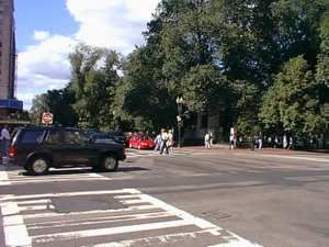
Object categ.     pLSA (a)     pLSA (b)     Fergus et al. [8]
   Faces                5.3          3.3             3.6
   Motorbikes          15.4          8.0             6.7
   Airplanes            3.4          1.6             7.0
   Cars rear*       21.4 / 11.9   16.7 / 7.0         9.7

Table 4: Equal error rates for image classification task for pLSA
and the method of [8]. Test images of a particular category were                            (a)                                  (b)
classified against (a) testing background images (test performed                     Topic                    P (topic|image)     # regions
                                                                                     1 Faces (yellow)               0.48             128
in [8]) and (b) testing background images and testing images of all
                                                                                     2 Motorbikes (green)           0.07               1
other categories. The improved performance in (b) is because our                     3 Airplanes (black)            0.00               0
method exhibits very little confusion between different categories.                  4 Cars rear (red)              0.03               0
(*) The two performance figures correspond to training on 400 /                      5 Backg I (magenta)            0.09               1
900 background images respectively. In both cases, classification                    6 Backg II (cyan)              0.17              12
is performed against an unseen test set of road backgrounds (as                      7 Backg III (blue)             0.15              23
in [8]), which was folded-in. See text for explanation.                                                       (c)
                                                                             Figure 6: Image as a mixture of visual topics (Expt. (2)) using 7
ROC curve for the topic k. Equal error rates for the four                    learned topics). (a) Original frame. (b) Image as a mixture of a
object topics are reported in table 4.                                       face topic (yellow) and background topics (blue, cyan). Only el-
    Note that for Airplanes and Faces our performance is                     liptical regions with topic posterior P (z|w, d) greater than 0.8 are
similar to that of [8] despite the fact that our ‘training’ is               shown. In total 7 topics were learnt for this dataset which con-
unsupervised in the sense that the identity of the object in                 tained faces, motorbikes, airplanes, cars, and background images.
                                                                             The other topics are not significantly present in the image since
an image is not known. This is in contrast to [8], where each
                                                                             they mostly represent the other categories and other types of back-
image is labelled with an identity of the object it contains,                ground. (c) The table shows the mixture coefficients P (z|d) for
i.e. about 5×400 items of supervisory data vs. one label                     this particular image. In total there are 693 elliptical regions in this
(the number of topics) in our case.                                          image of which 165 (102 unique visual words) have P (z|w, d)
    In the case of motorbikes we perform worse than [8]                      above 0.8 (those shown in (b)). The topics assigned to visual
mainly due to confusion between motorbike images con-                        words, dependent on the other words in the analyzed image, cor-
taining a textured background and the textured background                    respond well to object categories.
topic. The performance on Cars rear is poor because Car
images are split between two topics in training (a similar                   P (zk |wi , dj ) greater than 0.8. There is an impressive align-
effect happens in Expt. (1) for K=6). This splitting can be                  ment of the words with the corresponding object areas of
avoided by including more background images. In order                        the image. Note the words shown are not simply those most
to make results comparable with [8], Cars rear images were                   likely for that topic. Rather, from Equation (3), they have
classified against a completely new background dataset con-                  high probability of that topic in this image. This is an exam-
taining mainly empty roads. This dataset was not seen in                     ple of overcoming polysemy – the probability of the partic-
the learning stage and had to be ‘folded-in’ which makes                     ular word depends not only on the probability that it occurs
the comparison on Cars rear slightly unfair to the topic dis-                within that topic (face, say) but also on the probability that
covery approach.                                                             the face topic has for that image, i.e. the evidence for the
                                                                             face topic from other regions in the image.
4.3. Segmentation                                                            Expt. (5) Image segmentation for faces. We now inves-
In this section we evaluate the image’s spatial segmenta-                    tigate how doublets (i.e. an additional vocabulary formed
tion discovered by the model fitting. As a first thought, it                 from the local co-occurrences of visual words) can improve
is absurd that a bag of words model could possibly have                      image segmentation (cf single visual words – singlets). To
anything useful to say about image segmentation, since all                   illustrate this clearly, we start with a two class image dataset
spatial information has been thrown away. However, the                       consisting of half the faces (218 images) and backgrounds
pLSA model delivers the posteriors                                           (217 images). The procedure for learning the doublets is as
                                                                             follows: a four topic pLSA decomposition is learnt for all
                             P (wi |zk )P (zk |dj )                          training faces and training backgrounds with 3 fixed back-
         P (zk |wi , dj ) = PK                          ,          (3)
                                                                             ground topics, i.e. one (face) topic is learnt in addition to the
                             l=1 P (wi |zl )P (zl |dj )
                                                                             three fixed background topics (learned by fitting 3 topics to
and consequently for a word occurrence in a particular doc-                  a separate set of 400 training background images, cf Expt.
ument we can examine the probability of different topics.                    (2)). A doublet vocabulary is then formed from the top 100
   Figure 6 shows an example of ‘topic segmentation’ in-                     visual words of the face topic. A second four topic pLSA
duced by P (zk |wi , dj ) for the case of Expt. (2) with 7                   decomposition is then learnt for the combined vocabulary
topics. In particular, we show only visual words with                        of singlets and doublets with the background topics fixed.

                                                                         6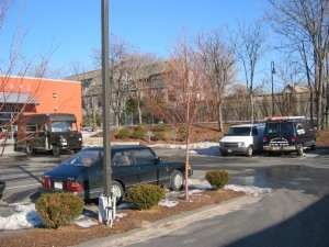
tions. Again all images have been converted to grayscale
                                                                         before processing.

                                                                         Topic discovery and segmentation: We fit pLSA with
                                                                         K = 10 topics to the entire dataset. The top 40 visual
          a                      b                      c                words from each topic are then used to form a doublet vo-
                                                                         cabulary of size 59,685. The pLSA is then relearned for a
                                                                         new vocabulary consisting of all singlets and all doublets.
                                                                         Figures 8 and 9 show examples of segmentations induced
                                                                         by 5 of the 10 learned topics. These topics, more so than the
          d                      e                      f                rest, have a clear semantic interpretation, and cover objects
Figure 7: Improving object segmentation. (a) The original frame          such as computers, buildings, trees etc. Note that the results
with ground truth bounding box. (b) All 601 detected elliptical          clearly demonstrate that: (i) images can be accessed by the
regions superimposed on the image. (c) Segmentation obtained by          multiple objects they contain (in contrast to GIST [14], for
pLSA on single regions. (d) and (e) show examples of ‘doublets’          example, which classifies an entire image); (ii) the topics in-
—locally co-occurring regions. (f) Segmentation obtained using           duce segmentations of multiple instances of objects in each
doublets. Note the extra regions on the right-hand side background       image.
of (c) are removed in (f).
The fixed background topics for the new combined vocabu-
lary are again pre-learnt on the separate set of 400 training
                                                                         5. Conclusions
backgrounds. The reason for running the first level single-              We have demonstrated that it is possible to learn visual ob-
ton pLSA is to reduce the doublet vocabulary to a manage-                ject classes simply by looking: we identify the object cat-
able size. Figure 7 compares segmentation on one example                 egories for each image with the high reliabilities shown in
image of a face using singlets and doublets.                             table 1, using a corpus of unlabelled images. Furthermore,
   The accuracy of the resulting segmentations is assessed               using these learnt topics for classification, we reproduce the
by comparing to ground truth bounding boxes (shown in                    experiments (training/testing) of [8], and obtain very com-
Figure 7a) for the 218 face images. Let GT and Rf be re-                 petitive performance – despite the fact that [8] had to pro-
spectively the set of pixels in the ground truth bounding box            vide about (400× number of classes) supervisory labels,
and in the union of all the ellipse regions labelled as face.            and we provide one label (number of topics).
The performance score ρ measures the area correctly seg-                    Visual words with the highest posterior probabilities for
mented by the word ellipses. It is the ratio of the intersection         each object correspond fairly well to the spatial locations
                                                        GT ∩R
of GT and Rf to the union of GT and Rf , i.e. ρ = GT ∪Rff .              of each object. This is rather remarkable considering our
This score is averaged over all face images to produce a sin-            use of the bag of words model. By introducing a second
gle number performance measure. The singleton segmenta-                  vocabulary built on spatial co-occurrences of word pairs,
tion score is 0.49, and the doublet segmentation improves                cleaner and more accurate segmentations are achieved.
this score to 0.61. A score of unity is not reached in prac-                The ability to learn topic probabilities for local appear-
tice because regions are not detected on textureless parts of            ances lets us apply the power and flexibility of unsupervised
the image (so there are always ‘holes’ in the intersection of            datasets to the task of visual interpretation.
the numerator). We have also investigated using doublets
composed from the top 40 visual words across all topics                  Acknowledgements: Financial support was provided by
(including background topics). In this case the segmenta-                the EC PASCAL Network of Excellence, IST-2002-506778,
tion score drops slightly to 0.59. So there is some benefit in           the National Geospatial-Intelligence Agency, NEGI-1582-
topic specific doublets.                                                 04-0004, and a grant from BAE Systems.
   Note the level of supervision to achieve this segmenta-
tion: the images are an unordered mix of faces and back-
grounds. It is not necessary to label which is which, yet
                                                                         References
both the face objects and their segmentation are learnt. The              [1] K. Barnard, P. Duygulu, N. de Freitas, D. Forsyth, D. Blei, and
supervision provided is the number of topics K and the sep-                   M. Jordan. Matching words and pictures. Journal of Machine Learn-
                                                                              ing Research, 3:1107–1135, 2003.
arate set of background images to pre-learn the background
topics.                                                                   [2] K. Barnard and D. Forsyth. Learning the semantics of words and
                                                                              pictures. In Proc. ICCV, 2001.
                                                                          [3] A. R. Barron and T. M. Cover. Minimum complexity density estima-
4.4. MIT image dataset results                                                tion. IEEE Trans. on Information Therory, 4:1034–1054, 1991.
MIT image data sets: The MIT dataset contains 2,873                       [4] D. Blei, A. Ng, and M. Jordan. Latent dirichlet allocation. Journal
images of indoor and outdoor scenes, with partial annota-                     of Machine Learning Research, 3:993–1022, 2003.

                                                                     7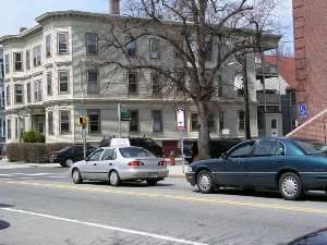
a

b

 c

d

                                                                                 Figure 9: Example segmentations on the MIT dataset for the 10
                                                                                 topic decomposition. Left: the original image. Middle: all de-
                                                                                 tected regions superimposed. Right: the topic induced segmen-
                                                                                 tation. Only topics a, b, c and d from figure 8 are shown. The
e                                                                                color key is: a-red, b-green, c-cyan, d-magenta. Note each image
                                                                                 is segmented into several ‘topics’.
                                                                                 [12] J. Matas, O. Chum, M. Urban, and T. Pajdla. Robust wide baseline
                                                                                      stereo from maximally stable extremal regions. In Proc. BMVC.,
Figure 8: Example segmentations induced by five (out of 10) dis-                      pages 384–393, 2002.
covered topics on the MIT dataset. Examples from the first 20                    [13] K. Mikolajczyk and C. Schmid. An affine invariant interest point
most probable images for each topic are shown. For each topic                         detector. In Proc. ECCV. Springer-Verlag, 2002.
the top row shows the original images and the bottom row shows                   [14] A. Oliva and A. Torralba. Modeling the shape of the scene: a holistic
visual words (doublets) belonging to that particular topic in that                    representation of the spatial envelope. IJCV, 42(3):145–175, 2001.
image. Note that we can give semantic interpretation to these top-               [15] A. Opelt, A. Fussenegger, and P. Auer. Weak hypotheses and boost-
ics: (a), (e) covers building regions in 17 out of the top 20 images;                 ing for generic object detection and recognition. In Proc. ECCV,
(b) covers trees and grass in 17 out of the top 20 images; (c) covers                 2004.
computers in 15 out of the top 20 images, (d) covers bookshelves                 [16] F. Schaffalitzky and A. Zisserman. Multi-view matching for un-
in 17 out of the top 20 images.                                                       ordered image sets, or “How do I organize my holiday snaps?”. In
                                                                                      Proc. ECCV, volume 1, pages 414–431. Springer-Verlag, 2002.
 [5] G. Csurka, C. Bray, C. Dance, and L. Fan. Visual categorization with        [17] H. Schneiderman and T. Kanade. A statistical method for 3D object
     bags of keypoints. In Workshop on Statistical Learning in Computer               detection applied to faces and cars. In Proc. CVPR, 2000.
     Vision, ECCV, pages 1–22, 2004.                                             [18] J. Sivic, B. C. Russell, A. Efros, A. Zisserman, and W. T. Free-
                                                                                      man. Discovering object categories in image collections. MIT AI
 [6] L. Fei-Fei, R. Fergus, and P. Perona. Learning generative visual mod-
                                                                                      Lab Memo AIM-2005-005, MIT, 2005.
     els from few training examples: An incremental bayesian approach
     tested on 101 object categories. In IEEE CVPR Workshop of Gener-            [19] J. Sivic and A. Zisserman. Video Google: A text retrieval approach
     ative Model Based Vision, 2004.                                                  to object matching in videos. In Proc. ICCV, 2003.
                                                                                 [20] Y. W. Teh, M. I. Jordan, M. J. Beal, and D. M. Blei. Hierarchical
 [7] L. Fei-Fei and P. Perona. A bayesian hierarchical model for learning
                                                                                      dirichlet processes. In Proc. NIPS, 2004.
     natural scene categories. In Proc. CVPR, 2005.
                                                                                 [21] A. Torralba, K. P. Murphy, and W. T. Freeman. Contextual models
 [8] R. Fergus, P. Perona, and A. Zisserman. Object class recognition by              for object detection using boosted random fields. In NIPS ’04, 2004.
     unsupervised scale-invariant learning. In Proc. CVPR, 2003.
                                                                                 [22] http://www.robots.ox.ac.uk/˜vgg/research/
 [9] T. Hofmann. Probabilistic latent semantic indexing. In SIGIR, 1999.              affine/.
[10] T. Hofmann. Unsupervised learning by probabilistic latent semantic          [23] P. Viola and M. Jones. Rapid object detection using a boosted cas-
     analysis. Machine Learning, 43:177–196, 2001.                                    cade of simple features. In Proc. CVPR, 2001.
                                                                                 [24] M. Weber, M. Welling, and P. Perona. Unsupervised learning of
[11] D. Lowe. Object recognition from local scale-invariant features. In
                                                                                      models for recognition. In Proc. ECCV, pages 18–32, 2000.
     Proc. ICCV, pages 1150–1157, 1999.

                                                                             8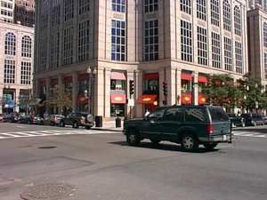
You can also read