Improving Accuracy of Nuclei Segmentation by Reducing Histological Image Variability - bioRxiv
←
→
Page content transcription
If your browser does not render page correctly, please read the page content below
bioRxiv preprint first posted online Apr. 6, 2018; doi: http://dx.doi.org/10.1101/296806. The copyright holder for this preprint
(which was not peer-reviewed) is the author/funder, who has granted bioRxiv a license to display the preprint in perpetuity.
                                 It is made available under a CC-BY 4.0 International license.

                      Improving Accuracy of Nuclei Segmentation by
                         Reducing Histological Image Variability
                                                    BMI 260 - Spring 2017

                                                   Yusuf Roohani? and Eric Kiss??

                                                            Stanford University

                              Abstract. Cancer is the second leading cause of death in United States.
                              Early diagnosis of this disease is essential for many types of treatment.
                              Cancer is most accurately observed by pathologists using tissue biopsy.
                              In the past, evaluation of tissue samples was done manually, but to im-
                              prove efficiency and ensure consistent quality, there has been a push to
                              evaluate these algorithmically. One important task in histological anal-
                              ysis is the segmentation and evaluation of nuclei. Nuclear morphology
                              is important to understand the grade and progression of cancer. Convo-
                              lutional neural networks (CNN) were used to segment train models for
                              nuclei segmentation. Stains are used to highlight cellular features. How-
                              ever, there is significant variability in imaging of stained slides due to
                              differences in stain, slide preparation and slide storage. This make auto-
                              mated methods challenging to implement across different datasets. This
                              paper evaluates four stain normalization methods to reduce the vari-
                              ability between slides. Nuclear segmentation accuracy was evaluated for
                              each normalized method. Baseline segmentation accuracy was improved
                              by more than 50% of its base value as measured by the AUC and Re-
                              call. We believe this is the first study to look at the impact of four stain
                              normalization approaches (histogram equalization, Reinhart, Macenko,
                              Khan) on segmentation accuracy.
                              Keywords: histopathology, CNN, machine learning, stain nor-
                              malization, nuclei segmentation

                     1      Introduction

                     Diagnoses made by pathologists using tissue biopsy images are central for many
                     tasks such as the detection of cancer and estimation of its current stage [2].
                     Known as histopathology, it is defined as the study of disease using microscopic
                     examination of a specimen processed with methods like dehydration, sectioning,
                     staining and fixed to a glass slide [6]. Recently, this analysis has become digital
                     with Whole Slide Imaging (WSI) allowing users to capture entire slides as colored
                     high resolution images [6]. It is important to note that color is especially impor-
                     tant in histopathology, since different stains are used to highlight cell structures.
                      ?
                          yroohani@stanford.edu
                     ??
                          erickiss@stanford.edu
bioRxiv preprint first posted online Apr. 6, 2018; doi: http://dx.doi.org/10.1101/296806. The copyright holder for this preprint
(which was not peer-reviewed) is the author/funder, who has granted bioRxiv a license to display the preprint in perpetuity.
                                 It is made available under a CC-BY 4.0 International license.

                     2

                     The intensities of the stains give different information due to interactions with
                     the cell components and metabolic processes.
                         One routine yet important step within histological analyses is the segmen-
                     tation of nuclei. Nuclear morphology is an important indicator of the grade of
                     cancer and the stage of its progression [3]. It has also been shown to be a pre-
                     dictor of cancer outcome [4] and counting mitosis events in nuclei is a useful
                     marker of cancerous growth. [2] Currently, histological analysis such as these are
                     done manually, with pathologists counting and evaluating cells by inspection.
                     Developing automated methods to perform this analysis will help pathologists
                     maintain consistent quality, allow for greater use of histological analysis by re-
                     ducing cost and throughput - particularly in longitudinal studies, and allow for
                     integration of results in electronic decision support systems.
                         However, automating nuclei detection is not a trivial task and can be chal-
                     lenging for a number of reasons. To fully understand the challenges, it is useful
                     to detail the image creation process. Tissue biopsies are taken from an area of
                     interest. The tissue is dehydrated, sectioned, stained, and photographed under a
                     high magnification microscope (20X-40X). A light source illuminates the bottom
                     of the sample and a sensor reads the relative absorption of the light through the
                     sample. Cell samples are typically clear, that is, they allow light to pass through
                     unaltered so stains are applied to the samples to allow for better differentiation
                     of key cellular features. Eosin and hematoxylin are commonly used stains with
                     the first staining nucleic acids a purple-blue and the latter staining proteins pink.
                         There are sources of error at each stage in the process. The tissue sample
                     itself may have clumped nuclei or dividing those that overlap. Stain manufac-
                     turing and aging can lead to differences in applied color. It could also be the
                     result of variation in tissue preparation (dye concentration, evenness of the cut,
                     presence of foreign artifacts or damage to the tissue sample), stain reactivity or
                     image acquisition (image compression artifacts, presence of digital noise, spe-
                     cific features of the slide scanner). Each stain has different absorption charac-
                     teristics(sometimes overlapping) which impact the resulting slide color. Finally,
                     storage of the slide samples can have aging effects that alter the color content.
                     However, unlike medical fields like radiology, digital approaches to histological
                     evaluation are fairly new so there isn’t always the same level of maturity in
                     comparing scans of different origin. [2] [5]
                         Radiologists have established standards (such as DICOM) to ensure con-
                     sistency between scans from different origins and time. Most relevant to this
                     project, DICOM data files, contain metadata that allow users to easily manipu-
                     late raw image values to standard units based on specific machine characteristics.
                     Ideally, histopathology would also work within a framework like DICOM where
                     images can be standardized against experimental condition to ensure consistency
                     across datasets.
                         The impact of such a standardization would be great. Aside from clinical and
                     research applications, standardizing image analysis solutions to handle histolog-
                     ical data from a variety of sources would also be valuable to the pharmaceu-
                     tical industry. Recently, there has been considerable interest in the application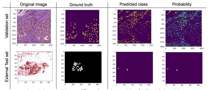
bioRxiv preprint first posted online Apr. 6, 2018; doi: http://dx.doi.org/10.1101/296806. The copyright holder for this preprint
(which was not peer-reviewed) is the author/funder, who has granted bioRxiv a license to display the preprint in perpetuity.
                                 It is made available under a CC-BY 4.0 International license.

                                                                                                                          3

                     of novel machine learning tools such as deep learning to aid in segmentation.
                     Some have used grayscale images to perform automated slide analysis, but this
                     ignores a deep source of data available from the stains. Color-based models gen-
                     erally work on raw pixel values, but could achieve greater accuracy through
                     reducing the variance contributed by slide and stain specific variables. However,
                     the approach must not be too general or else false positives will occur through
                     reduction or altering the image signal. [1] [3]

                     2     Methods

                     Fig. 1. This is a schematic overview of our overall approach. We first used a direct
                     histogram analysis to analyze the impact of stain normalization. We then trained a deep
                     learning model on one dataset and tested it on another. We performed segmentation
                     both before and after stain normalization to assess impact

                         The aim of this project is to address the impact of variability in histological
                     images on the accuracy of segmentation algorithms. Image statistics were found
                     on the raw images, and a CNN for nuclei segmentation was trained and tested
                     to get a baseline. Four stain normalization techniques, histogram equalization,
                     Reinhard, Macenko, and Kahn were then applied as means to reduce color vari-
                     ability of the raw images. The CNN was trained and tested again to get a final
                     segmentation accuracy. This paper is unique in that it employs a wide variety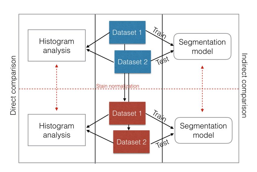
bioRxiv preprint first posted online Apr. 6, 2018; doi: http://dx.doi.org/10.1101/296806. The copyright holder for this preprint
(which was not peer-reviewed) is the author/funder, who has granted bioRxiv a license to display the preprint in perpetuity.
                                 It is made available under a CC-BY 4.0 International license.

                     4

                     of normalization methods, uses nuclei segmentation accuracy a metric, and tests
                     the model on a different dataset to understand model generalizability.

                     3     Dataset
                     Multiple publicly available datasets were used in this analysis. 58 histological
                     breast images were taken from the UCSB Bio-segmentation benchmark dataset.
                     Each RGB image is 896x768 pixels was H&E stained and included a correspond-
                     ing malignant or benign label. Manually annotated segmentation masks are also
                     provided as a ground truth. 143 breast images were also used from the Case
                     Western Reserve digital pathology dataset. Each RGB image was 2000x2000
                     pixels and was H&E stained. Manually annotated masks were provided for over
                     12000 nuclei.
                         These datasets were chosen because there were large differences in the resolu-
                     tion, color profile, and slide preparation quality. Obtaining such different images
                     highlighted the problem facing automation, but also offered an opportunity to
                     evaluate whether the segmentation classifier is generalizable outside of its train-
                     ing and validation set.

                     4     Stain Color Normalization
                     Stain normalization techniques involve transforming image pixel values. There
                     are a wide array of techniques in literature, but most involve statistical trans-
                     formations of images in various color spaces. This paper provides an overview of
                     the four techniques used.
                         University of Warwick’s normalization Matlab toolbox contained example
                     implementations of many of these techniques and served as the foundation for
                     processing the training and test datasets. A training image was selected for
                     training and test processing by inspection.

                     4.1     Histogram equalization
                     Histogram equalization is a commonly used image processing technique that
                     transforms one histogram by spreading out its distribution to increase image
                     contrast. In this analysis, histogram equalization was performed on each RGB
                     channel in Matlab, effectively normalizing the color intensities frequencies be-
                     tween two images. However, histogram equalization is known to increase the
                     contrast of noise and introduce artifacts since the assumption that the propor-
                     tion of stains is constant between the images[kahn].

                     4.2     Macenko color normalization
                     The Macenko color normalization method transforms the images to a stain color
                     space by estimating the stain vectors then normalizes the stain intensities. Quan-
                     tifying the stain color vectors (the RGB contribution of each stain) provides a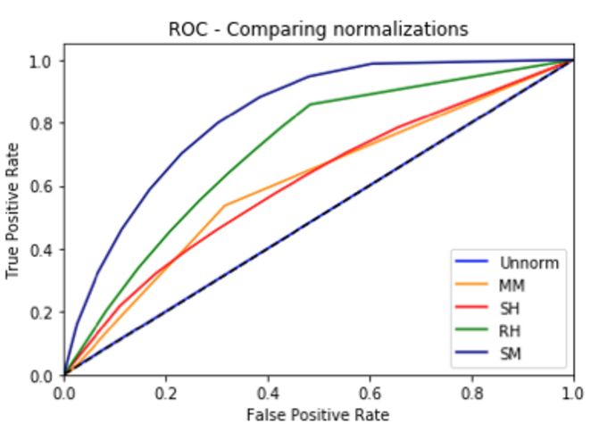
bioRxiv preprint first posted online Apr. 6, 2018; doi: http://dx.doi.org/10.1101/296806. The copyright holder for this preprint
(which was not peer-reviewed) is the author/funder, who has granted bioRxiv a license to display the preprint in perpetuity.
                                 It is made available under a CC-BY 4.0 International license.

                                                                                                                          5

                     more robust means of manipulating color information. However, due to the vari-
                     ability of stains discussed previously, an automated method to determine the
                     stain vectors is advised.
                         Macenko implements a method for automatic stain vector creation by con-
                     sidering images in the OD (optical density) space. Resulting OD values are a
                     linear combination of the stain vectors. Low OD values are also thresholded to
                     improve performance since background is considered to have an OD of 0. The
                     largest OD values are found via a single value decomposition (SVD). A plane
                     is calculated from the largest maximum values found, and the remainder of OD
                     pixels are projected onto this plane with their vector lengths normalized to unit
                     length. The angle of each point with respect to the first stain vector is calculated.
                     To account for noise, the 1st and 99th percentile of pixels for each value are used
                     to ensure a valid extremes. The extremes are then converted back to OD space.
                     Intensity variation is corrected for each stain. An intensity histogram is plotted
                     and the 99th percentile used as the maximum to account for noise. The target
                     image stain intensity histograms are then scaled to the source maximum.
                         This method has been criticized for altering fully saturated and empty OD
                     values during transformation and for altering the OD of both source and target
                     images[kahn].

                     4.3     Reinhard color normalization

                     Reinhard color normalization aims to make one image ’feel’ like another by
                     transforming one image distribution to be closer to another. Reinhard transforms
                     the target and source images into l” color space. In RGB color space, color
                     channels typically have a high degree of correlation (ie. if there is blue there is
                     likely green). Thus, any modifications to pixel values should have some impact
                     on the other channels. L” color space was created to minimize the correlation
                     between channels for natural scenes. L is an achromatic channel and while ” are
                     opposing Yellow-Blue and Red-Green channels.
                         After the source and target images are in L” colorspace, descriptive statistics
                     are used to transform the target image’s’ colorspace. For each channel, the mean
                     value is subtracted from the data points and the data points are scaled by the std
                     of the target/std of the source. Finally, the average channel values of the source
                     are added back to the data points. For images that are very different(a lot of sky
                     vs a lot of grass), the above method does not produce accurate results. Reinhard
                     suggests additional statistical methods to deal with widely varying images.
                         Instead of computing mean and standard deviation for on each channel for
                     the entire image, the statistics are calculated for scene swatches or clusters (ie
                     sky and grass). The distances are calculated to each cluster and divided by the
                     standard deviation. The transformed pixels for each cluster are weighted by the
                     normalized distances to produce a final output color. The technique easily scales
                     if there are greater than two clusters. After the color transformation in L” color
                     space, it is transformed back to RGB colorspace.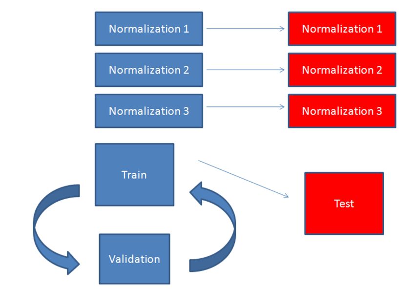
bioRxiv preprint first posted online Apr. 6, 2018; doi: http://dx.doi.org/10.1101/296806. The copyright holder for this preprint
(which was not peer-reviewed) is the author/funder, who has granted bioRxiv a license to display the preprint in perpetuity.
                                 It is made available under a CC-BY 4.0 International license.

                     6

                     4.4     Kahn color normalization

                     Conceptually, the Kahn normalization technique is similar to the Macenko tech-
                     nique in that it estimates the stain vectors, deconvolve the image, maps the stain
                     intensity to a target image, before reconstructing back in RGB colorspace. Kahn
                     makes contributions in automatic stain vector calculation using a classifier with
                     global and local pixel value information, and a non-linear stain normalization
                     method.
                         The stain classifier uses SCD to split up image into color batches using oct-
                     tree quantization. The SCD has its dimensionality reduced via principal compo-
                     nent analysis as a color description of the full image, encompassing information
                     on the stains. A relevance vector machine (RVM) supervised classifier had the
                     best performance. It was also found that without the global SCD information,
                     the classifier assigned significant probability to only weakly stained classes.
                         Optical density values are analyzed for each channel after being separated by
                     the classifier (stains, and background). Statistics were calculated for the stain
                     channel distributions with OD outliers excluded. A spline function was then
                     created to map the channel statistics of one image to another. The spline ensures
                     was created to ensure that the maximum and minimum OD remain unchanged
                     through the mapping. After the transformation the image is converted by the
                     RGB colorspace.

                     Fig. 2. Comparison of stain normalization techniques on a sample training image.
                     Source image was normalized to reference image using histogram equalization, Rein-
                     hard, Macenko, and Kahn methods respectively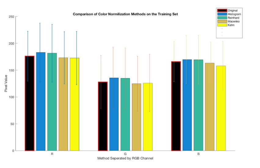
bioRxiv preprint first posted online Apr. 6, 2018; doi: http://dx.doi.org/10.1101/296806. The copyright holder for this preprint
(which was not peer-reviewed) is the author/funder, who has granted bioRxiv a license to display the preprint in perpetuity.
                                 It is made available under a CC-BY 4.0 International license.

                                                                                                                          7

                     5     Stain Normalization
                     Stain normalization techniques involve transforming image pixel values. There
                     are a wide array of techniques in literature, but most involve statistical trans-
                     formations of images in various color spaces. This paper provides an overview of
                     the four techniques used. University of Warwickś normalization Matlab toolbox
                     contained example implementations of many of these techniques and served as
                     the foundation for processing the training and test datasets.

                     Fig. 3. Comparison of stain normalization techniques on Case Western Reserve training
                     set. Mean pixel value and standard deviation was calculated for each color channel
                     demonstrating a quantitative change in color composition and increased variance.

                     6     Image segmentation using CNNs
                     This section describes the methods used to generate classifier models. The goal
                     was to train a model using one dataset and to test using another. We aimed to
                     perform this approach using different normalization strategies to narrow down
                     on an approach that best reduced variability and improved performance

                     6.1     Model selection
                     We first trained and validated the model on the same dataset to make sure that
                     our training procedure was working correctly. For this we used breast tissue slices
bioRxiv preprint first posted online Apr. 6, 2018; doi: http://dx.doi.org/10.1101/296806. The copyright holder for this preprint
(which was not peer-reviewed) is the author/funder, who has granted bioRxiv a license to display the preprint in perpetuity.
It is made available under a CC-BY 4.0 International license.
8
Fig. 4. Outline of model validation and testing procedure
from [3]. We split the dataset into 70% train and 30% validation. We then tried a
number of different network architectures, dataset augmentation techniques and
patch selection strategies to narrow down on a working approach. These efforts
have been briefly outlined in Table X. We chose to use a fully convolutional
network instead of a regular fully connected network to enhance throughput and
quickly retune the network based on results. We used the Caffe deep learning
framework to design these models. The final architecture that was chosen after
the validation procedure for this problem was (Conv-BNorm-ReLU)x6 - (Full
ConV) - Softmax [3]. It has extra convolutional layers as compared to a reg-
ular Alexnet but only one ’fully connected’ layer (that has in this case been
transformed into a fully convolutional layer).
6.2 Training Dataset
The training dataset consisted of histological sections of breast tissue. These
were all standardized at a resolution of 2000x2000 and a magnification of 20x.
We sampled patches from these images in order to develop a pixel level classifier.
Patch sizes of 32x32 and 64x64 were experimented with, and we found that a
patch size of 64x64 worked best for training. Some of the models experimented
with have been listed in Table X.
However, on training we realized that randomly sampling from non-nuclear
regions as defined by the hand annotations was not sufficient. This is becausebioRxiv preprint first posted online Apr. 6, 2018; doi: http://dx.doi.org/10.1101/296806. The copyright holder for this preprint
(which was not peer-reviewed) is the author/funder, who has granted bioRxiv a license to display the preprint in perpetuity.
It is made available under a CC-BY 4.0 International license.
9
the annotation mask only accounted for a subset of all the nuclei in the image.
Thus, there was a significant probability of sampling unannotated nuclei while
developing patches for the training set. To address this problem, we used the
approach outlined by [3]. Nuclei are known to absorb greater levels of the eosin
(red) stain and so the red channel in the images was enhanced. A negative mask
was thus generated defining regions outside of these enhanced red zones that
were deemed safe for non-nuclei class patch selection. We also made sure to
allocated a third of the non-nuclei patches to boundaries around the nuclei. This
ensured that the algorithm was careful to clearly mark out these boundaries and
not club nuclei together. The model prediction accuracy benefitted from both
these approaches.
The test set was composed also of breast tissue slices from a dataset provided
by the BioImaging lab at UCSB [link]. These were of a much smaller resolution
(896 x 768) and are referred to as the the BioSegmentation benchmark. This
dataset proved to be exceptionally useful for this problem because the images
were quite different from our training set both in terms of image quality and reso-
lution and also in terms of the staining used (more eosin content). This was ideal
for our approach since we could see how well the features learnt on a moderately
different dataset could transfer to this problem, and most importantly how we
could augment that process through better normalization and standardization.
Patching was not required for the test set because we were using a fully
convolutional network. This meant that our model could simply process an entire
image in one pass instead of needing it to be broken down into pixelwise patches
which involves a lot of redundant and time consuming computation. We used
the approach first described by [15].
6.3 Training
Once our model architecture and dataset generation approach had been final-
ized, we began to train separate model for each of the normalization scenarios as
shown in Fig 4. We used a batch size of 1000 because that could fit comfortably
in our memory (P100 GPU 16GB x 2) and also leave enough room for sharing
with other runs. Any further increases in batch size would not result in a per-
formance increase because of memory bandwidth limitations. We initially tested
architectures with a considerably large dataset of 2,500,000 images. However, we
soon realized that there was a critical flaw in how the binary LMDB databases
were being generated which was corrupting all those values, thus we chose to
use a slower I/O procedure and a smaller dataset. Since the images from which
patching was performed were still the same, we did not feel that the results would
be adversely affected by this. From previous experience, the authors expect that
merely oversampling from the same dataset would have improved accuracy by
not more than a few percentage points, whereas more structured sampling like
generating a negative annotation mask as described previously can have a more
significant impact.
Most of the models would quickly converge within 5-10 epochs. We allowed
each normalization model to run up to 25 epochs just to be sure. There werebioRxiv preprint first posted online Apr. 6, 2018; doi: http://dx.doi.org/10.1101/296806. The copyright holder for this preprint
(which was not peer-reviewed) is the author/funder, who has granted bioRxiv a license to display the preprint in perpetuity.
It is made available under a CC-BY 4.0 International license.
10
four models - these corresponded to the four techniques outlined previously:
Histogram Equalization (SH), Macenko (MM), Reinhard (RH), Spline Mapping
(SM). There was a also of course a model for the unnormalized (Unnorm) case
7 Results
Results from the segmentation model were analyzed both visually and using
quantitative metrics.
7.1 Visual inspection
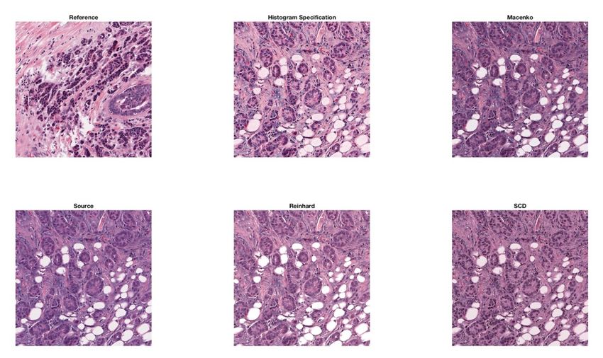
The top row in Fig 6 shows the original images after being transformed using the
four different stain normalization approaches. We can see that all four images
appear different in some respect. For example, HE and RH, which involve stain
normalization through working directly with the color values show a noticeable
blue tint. This is more pronounced in HE, where non-nuclear regions in the top
right of the cell get quite heavily stained with hematoxylin. On the other hand,
SM and RH, which both use stain vectors to map an input image to a target
space, don’t show a blue-ish tint and provide a much more robust transformation
that is true to the semantic information of the parent image (eg: treating nuclei
and background regions distinctly)
The bottom row looks at the class probability for nuclear regions as predicted
by models trained on datasets that were each stain normalized differently. Clearly
all four normalized sets perform far better than the unnormalized dataset where
almost no nuclei were detected due to the drastic change in staining as compared
to what the model had been trained on. HE does pick up most of the nuclei but
also a lot of background noise due to its inability to differentiate clearly between
different types of staining. RH is also more sensitive to noise but does a better
and clearer detection of nuclei as is visible in the clear boundaries. SM clearly
performs the best at segmenting nuclei while also being most robust to false
positives.
7.2 Quantitative assessment
To perform a more rigorous quantitative assessment, we looked at a range of
different metrics calculated over a randomly selected set of 15 test images. This
was essential because simply calculating classification accuracy would be insuffi-
cient for this sort of segmentation problem. For instance, even if a classifier were
to only classify pixels as non-nuclear regions it would still be around 85-90%
accurate because the vast majority of pixels don’t lie within nuclei. Thus, the
range of metrics that we calculated helped to characterize model performance
from many different perspectives.
Given the set of all nuclear pixels in the set, recall tells us what fraction of
those were picked up by the model. Clearly SM does a great job in this area.
SH and RH also do well but when we look at their precision values they arebioRxiv preprint first posted online Apr. 6, 2018; doi: http://dx.doi.org/10.1101/296806. The copyright holder for this preprint
(which was not peer-reviewed) is the author/funder, who has granted bioRxiv a license to display the preprint in perpetuity.
It is made available under a CC-BY 4.0 International license.
11
Fig. 5. Comparison of normalized and unnormalized models
Fig. 6. Comparison of different stain normalization procedures on model performance
on test setbioRxiv preprint first posted online Apr. 6, 2018; doi: http://dx.doi.org/10.1101/296806. The copyright holder for this preprint
(which was not peer-reviewed) is the author/funder, who has granted bioRxiv a license to display the preprint in perpetuity.
It is made available under a CC-BY 4.0 International license.
12
not as high as those for SM. Precision measures how many of the positives that
you picked up were actually relevant. This indicates the tendency of SH and
RH to pick up more false positives than SM. This trade-off between true and
false positives is best captured by the ROC curve (Fig 7). Here, we see that
the unnormalized case doesn’t add any value at all while all the normalization
scenarios show improved prediction accuracies. SM is the clear winner showing
an excellent range of operation at a TPR of ¿80/90% while only allowing an
FPR of 50%. This is very impressive considering how the model was trained on
a staining visually very different from the one in the test data. This difference
is quantiatively captured by the AUC. Finally, the F-score is another attempt
to capture segmentation accuracy without getting bogged down by all the true
negatives. It calculates the intersection of pixels that have been classified as
nuclei in both the prediction and the ground truth and it divides that over the
union of all pixels classified as nuclei by either set. Again, SM is seen to be the
best at improving accuracy of the algorithm.
Fig. 7. ROC Curve for models trained using different stain normalization schemes
While we aimed to run the same number of epochs for the same images for
all the (4+1) normalization scenario models that we were testing, due to time
constraints before the presentation we ran a few models for lesser than 25 epochs.
As we attempted to update the accuracy numbers with newer figures, it led to an
interesting finding that the accuracy tended to decrease with increasing numberbioRxiv preprint first posted online Apr. 6, 2018; doi: http://dx.doi.org/10.1101/296806. The copyright holder for this preprint
(which was not peer-reviewed) is the author/funder, who has granted bioRxiv a license to display the preprint in perpetuity.
It is made available under a CC-BY 4.0 International license.
13
Fig. 8. Quantitative comparison of model performance where training data has under-
gone different stain normalization procedures
of epochs. This is quite possible given that increased number of epochs leads to a
greater chance of overfitting to the training dataset. The goal of our approach is
to develop a generalizable approach to move across datasets and so it would be
more sensitive to overfitting than a regular model that works on similar looking
images.
8 Discussion
Through this study, we have explored several stain normalization approaches
that were all shown to reduce inter slide variability. The results (particularly
AUC, F-score) clearly indicate that using a stain normalization approach in-
creases the performance of the deep learning based segmentation algorithm. We
found that SM performed better than all other approaches. We believe this is
because it use a non-linear mapping function that is more accurate than the
other approaches. It is able to delineate between different regions and map them
appropriately to the target space.
We also noticed that the model seems to perform more poorly in case of
normalizations that tend to be biased more towards the eosin channel. In future,
it may make sense to normalize the stain of the training dataset using two dif-
ferent approaches. This would push the model to become robust to these subtle
changes and be less dependent on any one channel. In fact, this could also be
looked at as a regularization approach to enhance generalizability of deep learn-
ing based models in this space and prevent overfitting. On the other hand, we
must remain conscious of the fact that staining color is a very valuable source ofbioRxiv preprint first posted online Apr. 6, 2018; doi: http://dx.doi.org/10.1101/296806. The copyright holder for this preprint
(which was not peer-reviewed) is the author/funder, who has granted bioRxiv a license to display the preprint in perpetuity.
It is made available under a CC-BY 4.0 International license.
14
information in histological analyses and reducing the model’s recognition of crit-
ical differences would prove detrimental. Thus, there is a balance to be achieved
here.
9 Conclusion
In this study, we looked at the impact of stain normalization as a means of
reducing inter-dataset variability in histological sections and also as a way to
improve the accuracy of segmentation algorithms across datasets. We were able
to quantify improvements in both domains. To the best of our knowledge, this
is the first study that looks at all four of these techniques and assesses their
usability in the context of deep learning based segmentation models.
References
1. Ghaznavi, Farzad, et al. ”Digital imaging in pathology: whole-slide imaging and
beyond.” Annual Review of Pathology: Mechanisms of Disease 8 (2013): 331-359.
2. Irshad, Humayun, et al. ”Methods for nuclei detection, segmentation, and classi-
fication in digital histopathology: a review’current status and future potential.”
IEEE reviews in biomedical engineering 7 (2014): 97-114.
3. Janowczyk, Andrew, and Anant Madabhushi. ”Deep learning for digital pathol-
ogy image analysis: A comprehensive tutorial with selected use cases.” Journal of
pathology informatics 7 (2016).
4. Basavanhally A, Feldman M, Shih N, et al. Multi-field-of-view strategy for image-
based outcome prediction of multi-parametric estrogen receptor-positive breast
cancer histopathology: Comparison to Oncotype DX. Journal of Pathology Infor-
matics. 2011;2:S1. doi:10.4103/2153-3539.92027.
5. Khan, Adnan Mujahid, et al. ”A nonlinear mapping approach to stain normal-
ization in digital histopathology images using image-specific color deconvolution.”
IEEE Transactions on Biomedical Engineering 61.6 (2014): 1729-1738.
6. SABEENA BEEVI, K.; BINDU, G. R.. Analysis of Nuclei Detection
with Stain Normalization in Histopathology Images. Indian Journal of Sci-
ence and Technology, [S.l.], sep. 2015. ISSN 0974 -5645. Available at:
¡http://www.indjst.org/index.php/indjst/article/view/85321¿. Date accessed: 20
May. 2017. doi:10.17485/ijst/2015/v8i23/85321.
7. Reinhard, E., Ashikhmin, M., Gooch, B., & Shirley, P. (2001). Color transfer be-
tween images. IEEE Computer graphics and applications, 21(5):34-41.
8. Macenko, M., Niethammer, M., Marron, J. S., Borland, D., Woosley, J. T., Guan,
X., Schmitt, XC., & Thomas, N. E. (2009, June). A Method for Normalizing His-
tology Slides for Quantitative Analysis. In ISBI (Vol. 9, pp. 1107-1110).
9. Sethi, Amit et al. ’Empirical Comparison of Color Normalization Methods for
Epithelial-Stromal Classification in H and E Images.’ Journal of Pathology Infor-
matics 7 (2016): 17. PMC. Web. 20 May 2017.
10. https://www.math.uci.edu/icamp/courses/math77c/demos/hist eq.pdf
11. http://www2.warwick.ac.uk/fac/sci/dcs/research/tia/software/sntoolbox
12. http://bioimage.ucsb.edu/research/bio-segmentationbioRxiv preprint first posted online Apr. 6, 2018; doi: http://dx.doi.org/10.1101/296806. The copyright holder for this preprint
(which was not peer-reviewed) is the author/funder, who has granted bioRxiv a license to display the preprint in perpetuity.
It is made available under a CC-BY 4.0 International license.
15
13. Paramanandam M, O’Byrne M, Ghosh B, Mammen JJ, Manipadam
MT, Thamburaj R, et al. (2016) Automated Segmentation of Nuclei
in Breast Cancer Histopathology Images. PLoS ONE 11(9): e0162053.
https://doi.org/10.1371/journal.pone.0162053
14. T. W. Freer and M. J. Ulissey, ’Screening Mammography with Computer-aided
Detection: Prospective Study of 12,860 Patients in a Community Breast Center,’
Radiology, vol. 220, no. 3, pp. 781’786, Sep. 2001.
15. Long, J., Shelhamer, E., & Darrell, T. (2015). Fully convolutional networks for se-
mantic segmentation. In Proceedings of the IEEE Conference on Computer Vision
and Pattern Recognition (pp. 3431-3440).You can also read