HIAPER Pole-to-Pole Observations (HIPPO): fine-grained, global-scale measurements of climatically important atmospheric gases and aerosols
←
→
Page content transcription
If your browser does not render page correctly, please read the page content below
Downloaded from http://rsta.royalsocietypublishing.org/ on November 1, 2015

                                                 Phil. Trans. R. Soc. A (2011) 369, 2073–2086
                                                                    doi:10.1098/rsta.2010.0313

    HIAPER Pole-to-Pole Observations (HIPPO):
     fine-grained, global-scale measurements of
        climatically important atmospheric
                 gases and aerosols
                    BY S. C. WOFSY*, THE HIPPO SCIENCE TEAM
               AND  COOPERATING MODELLERS AND SATELLITE TEAMS†
                       Harvard University, Cambridge, MA, USA

The HIAPER Pole-to-Pole Observations (HIPPO) programme has completed three of
five planned aircraft transects spanning the Pacific from 85◦ N to 67◦ S, with vertical
profiles every approximately 2.2◦ of latitude. Measurements include greenhouse gases,
long-lived tracers, reactive species, O2 /N2 ratio, black carbon (BC), aerosols and CO2
isotopes. Our goals are to address the problem of determining surface emissions, transport
strength and patterns, and removal rates of atmospheric trace gases and aerosols at global
scales and to provide strong tests of satellite data and global models. HIPPO data show
dense pollution and BC at high altitudes over the Arctic, imprints of large N2 O sources
from tropical lands and convective storms, sources of pollution and biogenic CH4 in the
Arctic, and summertime uptake of CO2 and sources for O2 at high southern latitudes.
Global chemical signatures of atmospheric transport are imaged, showing remarkably
sharp horizontal gradients at air mass boundaries, weak vertical gradients and inverted
profiles (maxima aloft) in both hemispheres. These features challenge satellite algorithms,
global models and inversion analyses to derive surface fluxes. HIPPO data can play a
crucial role in identifying and resolving questions of global sources, sinks and transport
of atmospheric gases and aerosols.
                        Keywords: monitoring; polar; atmospheric science

                                        1. Introduction

Future action on climate change requires us to be able to distinguish surface
emissions of greenhouse gases (GHGs) directly associated with human activities
from indirect effects of climate change and from natural variations. Measurements
of concentrations of GHGs (e.g. CO2 , CH4 and N2 O) and tracers (e.g. CO,
SF6 , O2 /N2 ) have been used to derive surface fluxes, and to attribute emissions
to human activity or natural processes, in a variety of conceptual frameworks
[1–6]. A common approach is to exercise atmospheric chemistry transport models
(ACTMs) to simulate concentrations of pollutants in time and space over the
globe, typically combining a priori surface emission flux fields, rates for chemical
*Author for correspondence (wofsy@fas.harvard.edu).

One contribution of 17 to a Discussion Meeting Issue ‘Greenhouse gases in the Earth system:
setting the agenda to 2030’.

                                               2073           This journal is © 2011 The Royal Society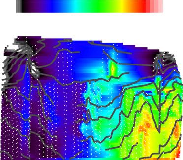
Downloaded from http://rsta.royalsocietypublishing.org/ on November 1, 2015

2074                                     S. C. Wofsy et al.

reactions in the atmosphere and assimilated meteorological fields. The surface
flux field is then adjusted to obtain the best match between model output and
data. The model is effectively ‘inverted’ to define optimal sources and sinks from
atmospheric concentrations.
   Global-scale ACTMs have difficulty resolving sharp chemical gradients, such
as exist at air mass boundaries, at the tropopause [7,8] or in plumes of tracers
emanating from strong source regions, a limitation inherent in the numerical
methods used in the Eulerian model framework [9]. ACTM outputs are commonly
compared with datasets that likewise do not resolve sharp gradients or define fine-
scale variance and covariance, e.g. data from sparse ground stations or satellites.
These data are in some respects ideal for comparison with global simulations,
since they may be presumed to represent large air masses and global-scale
processes. But, because accurate knowledge of vertical and horizontal gradients
is available neither from global data nor from global models, the fine-grained
structure of atmospheric tracer distributions is unknown and we have no way to
assess how important this structure might be for inverse models.
   Air mass boundaries move in space and time. Spatially aggregated data, or
measurements from widely spaced locations (e.g. remote island stations), give
horizontal patterns with diffuse boundaries. This fuzzy picture might be correct
if data are averaged over time (e.g. for a month), but the pattern is never
actually present in the atmosphere. A model may reproduce these smoothed
gradients with simulated rates of transport across air mass boundaries that are
significantly in error, leading to incorrect surface fluxes inferred from an inverse
analysis. Similarly, if the vertical gradient in a model is systematically in error,
the atmospheric mass burden (or column integral) is improperly simulated, and
significant bias can result when the model is inverted to obtain optimal surface
fluxes (e.g. [10]).
   Surface fluxes obtained by inverting global models are also subject to
systematic errors derived from other elements of the model framework, in addition
to transport errors. For example, misidentification of source processes and
locations, or incorrectly specified temporal variation of a priori fluxes, introduces
errors into ‘optimal’ flux fields associated directly with model constructs. Since
generally the only adjustable parameters in an inverse model are surface fluxes,
strong, independent tests of all elements of the model framework are needed,
using atmospheric measurements, in order to reduce the impact of these diverse
systematic errors and biases.
   This paper introduces the data obtained by the HIAPER Pole-to-Pole
Observations (HIPPO) project, a sequence of five global aircraft measurement
programmes that sample the atmosphere from (almost) the North Pole to the
coastal waters of Antarctica, from the surface to 14 km, spanning the seasons.
Three have been completed to date—January and November 2009, April 2010—
to be followed by June and August/September 2011 (denoted HIPPO-1, -2, etc.).
This paper will focus primarily on results obtained in HIPPO-1, for which data
have been finalized.
   HIPPO is intended to obtain global-scale, fine-grained data for the first time,
for a large number of atmospheric constituents. HIPPO data provide high-
resolution, systematic, pole-to-pole curtains with deeper vertical extent than
possible in the past, acquired at high temporal resolution to preserve correlations
among constituents. The goal is to provide new perspectives on how to use data

Phil. Trans. R. Soc. A (2011)
Downloaded from http://rsta.royalsocietypublishing.org/ on November 1, 2015

                         HIAPER Pole-to-Pole Observations (HIPPO)                          2075

to wring out transport issues in ACTMs, to identify and address the errors in the
spatial/temporal representation of surface fluxes and reaction rates, to discover
new features of trace gas and aerosol emissions and global-scale transport and to
rigorously test satellite algorithms. A related goal is to elucidate the underlying
processes and controls on surface emission fluxes, in order to be able to predict
emissions and atmospheric concentrations in the future.
   Fine-grained data have been obtained previously from aircraft platforms,
but only a few datasets have long transects covering extended time periods,
principally from commercial airliners that acquire data exclusively at cruise
altitude plus vertical profiles entering/leaving large urban complexes [11–13].
High-resolution datasets spanning the depth of the atmosphere over large areas
are available from a few surveys [14–17] that covered much smaller domains and
seasonal intervals than HIPPO. Thus, HIPPO data provide hitherto unavailable
information for testing and refining understanding of global distributions and
surface fluxes of trace gases and aerosols.

                     2. HIAPER Pole-to-Pole Observations payload

HIPPO measurements are summarized in table 1. The platform is the National
Science Foundation’s Gulfstream V (GV or HIAPER) aircraft operated by
the National Center for Atmospheric Research (NCAR). Major GHGs (CO2 ,
CH4 , N2 O) and other important trace species (CO, SF6 , O2 /N2 , H2 , etc.) were
measured at high frequency, many at 1 Hz, with two (or more) independent
measurements for each to provide redundancy (five for CO2 ), check calibration
and assess sensor drift. The quantum cascade laser spectrometer (QCLS), which
measures CO2 , CO, CH4 and N2 O, is a mid-infrared (IR) sensor developed by
Harvard University and Aerodyne Corp., owned by NCAR, and operated during
HIPPO by the Harvard team; the Observations of the Middle Stratosphere
(OMS) is a Harvard CO2 sensor using an IR gas analyser (IRGA), which has
logged more than 300 flights on airborne platforms [18]. The Research Aviation
Facility CO monitor (RAF-CO) refers to NCAR’s AeroLaser AL5002 vacuum–
UV sensor. Data at 1 Hz were obtained in two independent measurements for O3
and for H2 O (by the Vertical Cavity Surface Emitting Laser (VCSEL), a new
open path near-IR multi-pass spectrometer [19], and by the Unmanned Aircraft
Systems (UAS) Chromatograph for Atmospheric Trace Species (UCATS)-
H2 O, a National Oceanic and Atmospheric Administration (NOAA) mid-IR
spectrometer with a sampling inlet). AO2 is the NCAR Airborne Oxygen
Instrument, which measures O2 using a vacuum–UV absorption technique
[20] and CO2 using a single-cell IRGA (Licor 850). UCATS and the PAN
(PeroyAcylNitrate) and other Trace Hydrohalocarbon ExpeRiment (PANTHER)
are on-board gas chromatographs with extensive flight histories, measuring at
1–3 min intervals.
   A comprehensive suite of GHGs and a diverse ensemble of halocarbons,
hydrocarbons and sulphur species were measured by the whole-air sampler system
(WAS; [8]), using three different collection systems: stainless steel electropolished
cylinders (the Advanced Whole Air Sampler (AWAS) from the University of
Miami), glass vessels from the NOAA Programmable Flask Package (PFP)
programme (NWAS from NOAA) and special glass vessels for measuring O2 /N2

Phil. Trans. R. Soc. A (2011)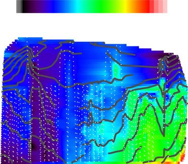
Downloaded from http://rsta.royalsocietypublishing.org/ on November 1, 2015

2076                                     S. C. Wofsy et al.

Table 1. Measurements and species on the GV in HIPPO. Bold font indicates species with three
                    or more measurements, sampling rates in parentheses.

Harvard/Aerodyne—HAIS QCLS              CO2 , CH4 , CO, N2 O (1 Hz)
NCAR AO2                                O2 /N2 , CO2 (0.5 Hz)
Harvard OMS CO2                         CO2 (0.5 Hz)
NOAA CSD O3                             O3 (1 Hz)
NOAA GMD O3 , H2 O                      O3 , H2 O (1 Hz)
NCAR RAF-CO                             CO (1 Hz)
NOAA UCATS and PANTHER                  CO, CH4 , N2 O, CFCs, HCFCs, SF6 , CH3 Br, PAN, CH3 Cl,
  gas chromatographs                      H2 , H2 O (1 sample per 70–200 s)
whole-air sampling: NWAS                O2 /N2 , N2 /Ar, CO2 , CH4 , CO, N2 O, other GHGs,
  (NOAA), AWAS (Miami),                   halocarbons, SF6 , H2 , COS, CS2 , solvent gases, reactive
  MEDUSA (NCAR/Scripps)                   hydrocarbons, marine species, isotopes of CO2 , etc.
VCSEL Princeton/SWS                     H2 O (1 Hz)
NOAA SP2                                BC mass, size (1 Hz)
MTP, wing stores                        T, P, vertical structure, winds, aerosols, cloud water

and Ar/N2 ratios and the isotopic composition of CO2 (Multiple Enclosure Device
for Unfractioned Sampling of Air (MEDUSA) from the University of California
at San Diego).
   BC was measured at 1 Hz by the NOAA single-particle soot photometer
(SP2) [21] on air drawn into the cabin. The SP2 uses a laser beam to heat
the BC component of individual fine-mode aerosol particles to vaporization,
resulting in emission of thermal radiation that is interpreted to give the BC
mass concentration and size distribution. Other particle probes, including a
cloud droplet probe (CDP), the NCAR Ultra High Sensitivity Aerosol Sampler
(UHSAS), the 2D-C particle imager and the PMS liquid water sensor (King)
(Precipitable Liquid Water Content (PLWC)), resided on the wing, along with
the microwave temperature profiler (MTP), which measures the temperature
profile above and below the plane, and a digital camera that acquired an image
every second.

                                             3. Results

Figure 1 shows the flight tracks for HIPPO-1 and -2, plus vertical sampling
and observed isentropic structure for HIPPO-1. Each deployment obtained a
southbound cross section of the atmosphere near the International Date Line,
covering the Arctic Ocean, Alaska and the entire Pacific to just short of
Antarctica. Northbound, HIPPO-1 traversed the South Pacific to sample in the
eastern tropical Pacific upwelling zone, and HIPPO-2 sampled the western Pacific
warm pool. We obtained 138, 151 and 136 vertical profiles in HIPPO-1, -2 and -3,
respectively, spanning 67◦ S–80◦ N. On average, consecutive samples in the mid-
troposphere are separated by 2.2◦ of latitude, with 4.4◦ between consecutive
near-surface or high-altitude samples. Most profiles extended from approximately
300 to 8500 m altitude, constrained by air traffic, but significant profiling extended
above approximately 14 km (figure 1c).

Phil. Trans. R. Soc. A (2011)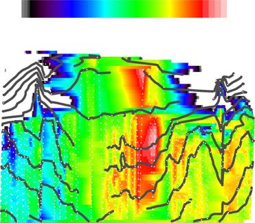
Downloaded from http://rsta.royalsocietypublishing.org/ on November 1, 2015

                                          HIAPER Pole-to-Pole Observations (HIPPO)                                                                    2077

        (a)                                                                           (b)
                         60

                         30
          latitude

                          0

                     −30

                     −60

                               150     −160     −110       −60                                            150         −160     −110                  −60
                                         longitude                                                                      longitude

                                                                                                                             (Q)
  (c)                                                                           (d)
                                                                                                          260          300          340        380
               15                                                                 15 000
                                                                                                                360           350          360
  P-ALT (km)

                                                                       altitude (m)
               10                                                                 10 000                                                   340

                                                                                                                      330
                     5                                                                5000                            320

                                                                                                 29                   310                      290
                                                                                                      0                       300
                 0                                                                          0
                              −50            0           50                                     −60               −20       0 20          40     60    80
                                          latitude                                                                      latitude

Figure 1. (a, b) Locations of flight tracks and vertical profiles (red points) for HIPPO deployments 1
and 2. (c) Vertical profiles in the HIPPO-1 cross section of the Pacific southbound near the date line
(flights 2–7), tropopause heights (pressure altitude (km); cyan) from MTP, and stratospheric flight
segments in red. (d) Cross section of potential temperature (Q) in HIPPO-1, on the southbound
leg near the date line. The white dotted lines mark the flight path of the GV, and grey lines show
contours of potential temperature. Altitudes are given in metres above sea level (m.a.s.l.) (GPS).
(Online version in colour.)

   Figure 1d shows the cross section of potential temperature (Q) versus latitude
and GPS altitude (m.a.s.l.) during HIPPO-1. A dome of very cold, stable air,
with a strong latitude gradient of Q, covered the Arctic, with a sharp transition
at the northern edge of the polar jet, near 60◦ N. There was a narrow zone of
stratospheric influx just equatorward of 60◦ N, and then a belt of much weaker
vertical stratification from 60◦ to 40◦ N, the region of the ‘warm conveyor belt’,
where vertical transport occurs in association with jet stream dynamics and mid-
latitude storms [22,23]. Equatorward of 40◦ N, there was a broad Q bulge in the
middle and upper troposphere, reflecting the influence of deep convection and
the Hadley circulation. The Southern Hemisphere (SH) had similar structure,
but the features were weaker, reflecting the summer season.
   Figure 2 shows cross sections along the date line for key species in January 2009
(HIPPO-1). Atmospheric tracers displayed sharp transitions in the horizontal,
demarcating the boundaries between polar, middle latitude, subtropical and

Phil. Trans. R. Soc. A (2011)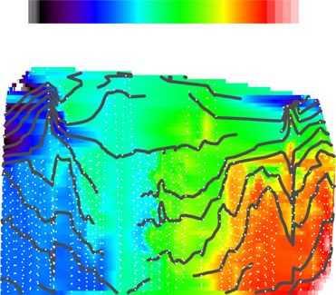
Downloaded from http://rsta.royalsocietypublishing.org/ on November 1, 2015
2078 S. C. Wofsy et al.
(a) (b)
1650 1750 1850 40 60 80 120 160
15 000
360 350 360 360 360
altitude (m)
10 000 340 340
330 330
5000 320 320
29 310 290 29
310 290
0 300 0 300
0
(c) (d)
382 386 390 394 6.1 6 .3 6.5 6 .7 6.9
15 000
360 350 360
360 350 360
altitude (m)
340
10 000 340
330
330
5000 320
320
310 290
310 290
29
29
0 300
0
0
(e) (f)
318 320 322 324 326 0.5 1 .5 2.5 3 .5 4.5
15 000
360 350 360 360 360
altitude (m)
10 000 340 340
330 330
5000 320 320
29 310 290 29 310 290
0 300 0 300
0
−60 −40 −20 0 20 40 60 80 −60 −20 0 20 40 60 80
latitude latitude
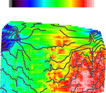
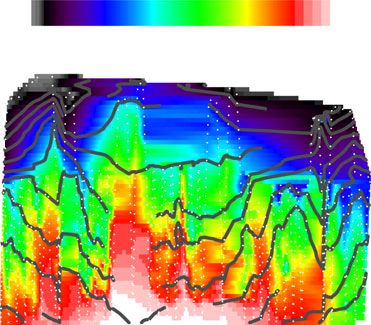
Figure 2. Cross sections of (a) CH4 (ppb), (b) CO (ppb), (c) CO2 (ppm), (d) SF6 (ppt), (e) N2 O
(ppb) and (f ) H2 O (log10 (ppm)) on HIPPO-1, southbound along the date line, January 2009.
White dotted lines show flight tracks, and grey contours show potential temperature. SF6 data
represent a composite of PANTHER and UCATS data, and H2 O data are from VCSEL. Altitudes
are given in m.a.s.l. (GPS). (Online version in colour.)
tropical air masses, and at the intertropical convergence zone (ITCZ; the
persistent line of convective storms that circles the globe near the equator,
demarcating the boundary between the hemispheres). Gradients were much
weaker in the vertical than in the horizontal, except in the northern polar
region where fresh inputs of CO, CO2 , CH4 and SF6 were evidenced by high
values near the surface and the presence of very short-lived pollutants (e.g.
Phil. Trans. R. Soc. A (2011)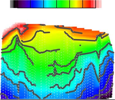
Downloaded from http://rsta.royalsocietypublishing.org/ on November 1, 2015

                         HIAPER Pole-to-Pole Observations (HIPPO)                          2079

benzene). According to model simulations (discussed further below), these
pollutants originated from Asia and Europe. In the Arctic, tracer isopleths
broadly aligned with isentropes, with sporadic anomalies owing to proximate
emissions or to stratospheric influence. Convective transport across isentropes
was evident elsewhere, in mid-latitudes, tropics and subtropics, particularly for
the longest lived tracers (e.g. SF6 and N2 O). The peak value of SF6 over the
North Pacific was observed in the middle troposphere. Concentrations of N2 O
showed a completely different pattern from other GHGs, with a prominent bulge
in the middle and upper tropical and subtropical troposphere, plus sporadic
enhancements between 10 and 14 km. Similar features were seen for N2 O in all
three missions flown so far.
   Water vapour showed the expected increases with temperature and tropical
origin. Input of very wet air was notable in the South Pacific convergence zone
(SPCZ; 10–20◦ S). The SPCZ is a persistent frontal formation of widespread cloud
cover and precipitation extending in a southeast direction from New Guinea into
the SH mid-latitudes, with strong convection typically extending over a large
area. It is specially prominent in boreal winter [24]. The SPCZ is spatially larger,
and contains more intense convection, than similar convergence zones elsewhere,
such as the South Indian Convergence Zone (SICZ) and the South Atlantic
Convergence Zone (SACZ), although it is not clear why [24]. Analogous, but
less distinct, anomalies have been observed for other chemical tracers near the
SPCZ [25,26]. In each of the three HIPPO missions so far, the water vapour
plume from the SPCZ has been larger in extent, and penetrated deeper into
the atmosphere, than in the ITCZ. These results suggest that the SPCZ may
be an important global source of water vapour to the tropical tropopause layer
over the Pacific, at least in the boreal winter season, supporting inferences
from observations of cirrus clouds over the tropical western Pacific during that
season [27].
   Figure 3 shows cross sections for HIPPO-2 in November 2009. Inverted vertical
profiles (i.e. with higher concentrations aloft) were surprisingly strong. Pollutant
levels typical of urban corridors were found in a thick layer at 6–8 km over
an extensive region of the Arctic, overlying clean air. The layers preserve
coherence (figure 3d,e) among tracers despite sharp gradients and transport over
thousands of kilometres, with strong vertical uplift. Very high levels of BC aerosol
were present, and absorption of solar radiation was visible (figure 3c). High
aerosol concentrations indicate the absence of efficient precipitation scavenging,
suggesting that polluted air was lofted by isentropic advection over the cold dome
that was in the process of developing over the Arctic. Notable enhancements of
N2 O were observed in some of the plumes. In many descents, enhanced CH4
concentrations were observed near the surface of the Arctic Ocean, sometimes in
otherwise pristine air, possibly signifying emission from biogenic sources or from
CH4 hydrates (e.g. figure 3c, below 2000 m). Horizontal gradients were again very
sharp at air mass boundaries.
   Figure 4 illustrates the meridional gradients of CO2 and O2 /N2 . Concentrations
of CO2 were enhanced above the surface (but not at the surface) from 45◦ S to
70◦ S in January (figures 2c and 4a), which might confirm a signal of elevated
CO2 in this region similar to that reported by the Atmospheric Infrared Sounder
(AIRS) satellite [28]; the structure of the CO2 distribution is rather complex,
with probable contributions from multiple processes including fires in Australia

Phil. Trans. R. Soc. A (2011)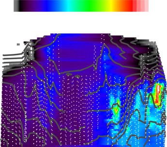
Downloaded from http://rsta.royalsocietypublishing.org/ on November 1, 2015

2080                                                                     S. C. Wofsy et al.

     (a)                                                                                 (b)
                                     381   383    385     387    389     391                           50         100     150       200     250
                   15 000
                                                                         370
    altitude (m)

                                     370 3                                                       370                                          370
                                           40                                                               340
                                                                       350                                                                 350
                   10 000

                                                   330                                                                  330
                    5000                            320                                                                 320
                                                           310                                                                310
                                                                  290
                                                   300                                                                  300
                             0
                                 −60        −20      0 20 40 60 80                             −60           −20 0 20 40 60 80
                                                   latitude                                                    latitude

                                                          (c)

                   (d)                                                             (e)                 386         387        388     389         390      391     392

        10 000 100                          150            200               250    10 000           324.4        324.6       324.8   325.0       325.2    325.4

                   8000                                                              8000

                   6000                                                              6000
  Z (m)

                   4000                                                              4000

                   2000                                                              2000

                         0                                                                0
                                 0    50 100 150 200 250                                             1860               1870              1880            1890
                                      black carbon (ng kg–1)                                                                    CH4

Figure 3. (a, b) Cross sections of CO2 (ppm) and CO (ppb), on HIPPO-2, southbound along the
date line, November 2009. Grey contours show potential temperature. (c) Photo of dense layer
of dark aerosols, looking north at 80◦ N, 8 km altitude, 2 November 2009 (photo: E. Kort). (d)
Vertical profiles of black carbon (BC) and CO at 77.2◦ N, on HIPPO-2, 2 November 2009. Black
lines, BC; red lines, CO. (e) Vertical profiles of CO2 , CH4 and N2 O at 77.2◦ N, on HIPPO-2, 2
November 2009. Black lines, CH4 ; green lines, CO2 ; blue lines, N2 O. (Online version in colour.)

Phil. Trans. R. Soc. A (2011)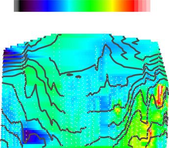
Downloaded from http://rsta.royalsocietypublishing.org/ on November 1, 2015

                                 HIAPER Pole-to-Pole Observations (HIPPO)                                 2081

         (a) 394                                             (b)

                     392
                                                                             −380
                     390

                                                              O2 (per meg)
         CO2 (ppm)

                     388
                                                                             −420
                     386

                     384
                                                                             −460
                     382
                             −50          0       50                                −50       0      50
                                      latitude                                            latitude

Figure 4. (a) Meridional gradients of CO2 averaged between 0.3 and 1.5 km and between 3.5 and
6.5 km. (b) Variation of the O2 : N2 ratio, as in (a). Green plus symbols, 0.3–1.5 km; open circles,
3.5–6.5 km. (Online version in colour.)

and uptake of CO2 at the ocean surface. There is excess O2 near the surface all
the way from 20◦ S to 60◦ S (figure 4b), reflecting inputs to the atmosphere from
both the ocean and the land, including thermal degassing of O2 from the ocean
and biological production of O2 from land and ocean in summer.
   Preliminary simulations of HIPPO-1 data have been made with global models
including Goddard Earth Observing System (GEOS) Chemical Tracer Model
(CHEM) [1], ACTM [6] and Global and regional Earth-system Monitor using
Satellite and in situ data/Monitoring and Forecasting Atmospheric Composition
(GEMS/MACC) [29]. Examples are shown in figure 5a–d. The models extracted
computed values along the flight track for detailed comparison with HIPPO.
Model simulations performed reasonably well in many respects, as can be seen by
comparing with figure 2. Simulations of CO2 from the GEOS-CHEM model ([30];
figure 5a) captured many features of the observations (figure 2), including the
relatively well-mixed profiles in subpolar and middle latitudes. Vertical contrasts
occurred mostly over the Arctic and Antarctic/Southern Ocean, reflecting inputs
from fossil fuels and marine biological uptake, respectively. But horizontal
gradients were much sharper in the atmosphere, and vertical gradients weaker,
than in the models. Most satellite data likewise do not resolve the observed
gradients. Enhanced CO2 poleward of 40◦ S seen by HIPPO is not reproduced
in the model; the major pollution signature appears at 60◦ N instead of 80◦ N;
enhanced surface CO2 in the SH deep tropics, probably from equatorial upwelling,
is not simulated in the model.
   Both the ACTM and GEOS-CHEM models appear to have vertical transport
rates that are too weak at high latitudes (compare CO2 , SF6 and CO in
figures 2–5), both along and across isentropes. The GEMS/MACC model gives a
somewhat better appearance for vertical profiles of CO and CH4 (not shown),
but has anomalies elsewhere and misses global-scale North–South gradients
significantly: GEMS/MACC predicts 70 ppb for DCO between the Antarctic and
the Arctic, compared with approximately 95 ppb observed.

Phil. Trans. R. Soc. A (2011)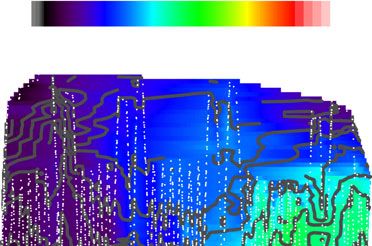
Downloaded from http://rsta.royalsocietypublishing.org/ on November 1, 2015

2082                                                             S. C. Wofsy et al.

 (a)                                                                                (b)

                15 000     382         386      390          394                                   15 000         6.3 6.4 6.5 6.6 6.7          6.8
                                     360                                                                                      370
                                 0                   360
                            37                                                                                                  350      360
 altitude (m)

                                                                                    altitude (m)
                                                            350
                10 000         0              340                                                  10 000                                  340
                            33
                                                           320          10                                                                  320
                                                                       3
                                                                                                                            330
                 5000                                                                               5000
                                                                                                                            310
                                                    300                    0
                                                                       27                                                          300
                    0                                                                                  0
                         −60          −20 0 20 40                 60           80                           −60        −20 0 20 40                60    80
                                         latitude                                                                         latitude

 (c)                                                                                (d)

            10 000                                                                                 15 000    318      320         322    324      326
                                                                                                                             370
                                                                                                                               350
 altitude (m)

                                                                                    altitude (m)
                                                                                                                                         360

                                                                                                   10 000                                  340
                6000                                                                                                                        320

                                                                                                                            330
                                                                                                    5000
                2000                                                                                                        310
                                                                                                                                   300
                    0                                                                                   0
                         322.5        323.5         324.5          325.5                                    −60        −20 0 20 40                60    80
                                              N2O                                                                         latitude

Figure 5. Model simulations for HIPPO-1, southbound along the date line, January 2009. (a,b)
Cross sections of CO2 (ppm) and SF6 (ppt) from the GEOS-CHEM and ACTM models,
respectively. (c) Vertical profiles of N2 O in the subtropics (ACTM and observed in HIPPO-1).
Blue filled squares, HIPPO-1; black open circles, ACTM. (d) Cross section for N2 O from the
ACTM for the HIPPO-1 flight track (flights 2–7). (Online version in colour.)

   HIPPO data for N2 O differ radically from model results. Simulations
completely miss the major feature of the global distribution, the tropical/sub-
tropical maxima at altitude (figure 5c,d), with greater enhancement north of
the ITCZ. This pattern has been observed in all six HIPPO cross sections
flown to date, although the magnitude of the enhancement aloft was largest in
HIPPO-1 southbound. HYSPLIT [31] trajectories showed that air near the surface
originated from the east, whereas the air with enhanced N2 O concentrations,
above 2 km, came from the west, suggesting sources in regions of convection in the
western Pacific and/or tropical South Asia or Indonesia. Samples collected on the
CARIBIC flights of commercial aircraft from Germany to India [32] also showed
diffuse maxima of N2 O in the upper troposphere (8.5–12 km) during June–August,
peaking in the same general latitude range as in HIPPO flights (15–25◦ N). It
appears that much of the excess N2 O seen by HIPPO was generated in the tropics,
but it is difficult to distinguish land-based sources from possible production by
corona discharge or lightning in convective storms [33] or by other mechanisms.

Phil. Trans. R. Soc. A (2011)
Downloaded from http://rsta.royalsocietypublishing.org/ on November 1, 2015
HIAPER Pole-to-Pole Observations (HIPPO) 2083
Previous studies [34,35] using sparse station data have already suggested that
unaccounted tropical sources were needed to close the N2 O budget. HIPPO data
strongly support that view. Elevated concentrations high in the atmosphere found
in HIPPO indicate a notably stronger tropical source than could be inferred from
surface data only. Even in the north polar region, HIPPO data often showed
maximum concentrations of N2 O aloft (cf. figures 2, 3 and 5), emphasizing the
difficulty of using surface measurements for modelling of this important species.
4. Summary and conclusions
HIPPO flights provide a unique dataset for atmospheric research: simultaneous,
fine-grained, global, high-frequency measurements of major GHGs, tracers with a
wide range of chemical lifetimes and diverse source processes, O2 /N2 and Ar/N2
ratios, BC and aerosols, plus the isotopic composition of CO2 . Concentration
data from HIPPO are linked to world standards, and multiple measurements
provide checks on data quality. The data from all missions will be publicly
available within 12–18 months of collection. HIPPO data have already played a
major role in calibrating total column measurements of CO2 , CO and CH4 from
the Total Carbon Column Observing Network (TCCON) of Fourier transform
spectrometers [36].
First impressions already highlight new phenomena: dense pollution high over
the Arctic in late autumn/early winter, with a notable component of BC; the
imprint of large N2 O sources in the tropical or subtropical areas of Asia or the
western Pacific and sources of CH4 in the Arctic both from fossil-fuel extraction
and from non-industrial sources. Although not discussed here, we also observed
short-lived gases emanating from various marine environments across the Pacific
(e.g. methyl nitrate, haloforms) and from major industrial areas.
HIPPO data clearly delineate the atmospheric imprint of summertime sinks for
CO2 and sources for O2 in the SH, providing a new tool to infer the strength of
ocean and land fluxes in the carbon cycle. Curtain plots reveal large-scale features
invisible to satellites and blurred by models, revealing the internal structure
of global CO2 distributions hitherto observed fuzzily by satellites and sparse
remote stations.
The most novel aspect of HIPPO is the imaging of the signatures of global
atmospheric transport modes with high clarity. From the SPCZ and ITCZ to the
cold dome over the winter pole, HIPPO data show the influence of convection,
isentropic transport and stratosphere–troposphere exchange, with fine resolution
at global scale. Remarkably sharp gradients in tracer concentrations are observed
at air mass boundaries. Inverted tracer gradients, with maxima aloft, were found
to be common in both hemispheres over the Pacific. These features present major
challenges to global models and to observation systems using sparse surface
stations and satellites. If not represented in global inverse model studies, they
can lead to major biases and inconsistencies. HIPPO data can play a crucial role
in identifying and resolving these issues.
The HIPPO Programme was supported by NSF grants ATM-0628575, ATM-0628519 and ATM-
0628388 to Harvard University, University of California (San Diego), University Corporation for
Atmospheric Research, University of Colorado/CIRES and by the NCAR. The NCAR is supported
by the National Science Foundation. Participation by several instruments (SP-2, Ozone, UCATS,
Phil. Trans. R. Soc. A (2011)Downloaded from http://rsta.royalsocietypublishing.org/ on November 1, 2015
2084 S. C. Wofsy et al.
PANTHER, NWAS flasks), and weather forecasting, were supported by offices and programmes
of the National Oceanic and Atmospheric Administration: the Atmospheric Composition and
Climate Programme, the Office of Oceanic and Atmospheric Research and the Environmental
Research Laboratory. The AWAS flasks system was supported by NSF grants NSF ATM0849086
and AGS0959853 to the University of Miami. VCSEL was supported by NSF grant AGS-1036275
to Princeton University. We are grateful to the crew of the GV for their dedication and professional
skill in making the flights possible and in taking the GV to places not previously visited by a jet
aircraft, and to the NCAR Earth Observing Laboratory for support of logistics and public outreach.
The authors gratefully acknowledge the NOAA Air Resources Laboratory (ARL) for the provision
of the HYSPLIT transport and dispersion model.
† S. C. Wofsy, B. C. Daube, R. Jimenez, E. Kort, J. V. Pittman, S. Park, R. Commane, B.
Xiang, G. Santoni, D. Jacob, J. Fisher, C. Pickett-Heaps, H. Wang, K. Wecht, Q.-Q. Wang (School
of Engineering and Applied Science, Harvard University, Cambridge, MA, USA); B. B. Stephens, S.
Shertz, P. Romashkin, T. Campos, J. Haggerty, W. A. Cooper, D. Rogers, S. Beaton, R. Hendershot
(National Center for Atmospheric Research, Boulder, CO, USA); J. W. Elkins, D. W. Fahey, R.
S. Gao, F. Moore, S. A. Montzka, J. P. Schwarz, D. Hurst, B. Miller, C. Sweeney, S. Oltmans,
D. Nance, E. Hintsa, G. Dutton, L. A. Watts, J. R. Spackman, K. H. Rosenlof, E. A. Ray, B.
Hall (NOAA ESRL and CIRES, Boulder, CO, USA); M. A. Zondlo, M. Diao (Department of
Civil and Environmental Engineering, Princeton University, Princeton, NJ, USA); R. Keeling, J.
Bent (Scripps Institution of Oceanography, University of California at San Diego, CA, USA); E. L.
Atlas, R. Lueb (Rosenstiel School of Marine and Atmospheric Science, University of Miami, Miami,
FL, USA); M. J. Mahoney, M. Chahine, E. Olsen (Jet Propulsion Laboratory, Pasadena, CA,
USA); P. Patra, K. Ishijima (Research Institute for Global Change, JAMSTEC, Yokohama, Japan);
R. Engelen, J. Flemming (European Centre for Medium-Range Weather Forecasts, Reading, UK);
R. Nassar, D. B. A. Jones (Department of Physics, University of Toronto, Toronto, Canada);
S. E. Mikaloff Fletcher (National Institute for Water and Atmospheric Research, Wellington,
New Zealand).
References
1 Bey, I. et al. 2001 Global modeling of tropospheric chemistry with assimilated meteorology:
model description and evaluation. J. Geophys. Res. Atmos. 106, 23 073–23 095. (doi:10.1029/
2001JD000807)
2 Engelen, R. J., Serrar, S. & Chevallier, F. 2009 Four-dimensional data assimilation of
atmospheric CO2 using AIRS observations. J. Geophys. Res. 114, D03303. (doi:10.1029/
2008JD010739)
3 Gurney, K. R. et al. 2002 Towards robust regional estimates of CO2 sources and sinks using
atmospheric transport models. Nature 415, 626–630. (doi:10.1038/415626a)
4 Kort, E. A. et al. 2008 Emissions of CH4 and N2 O over the United States and Canada based on
a receptor-oriented modeling framework and COBRA-NA atmospheric observations. Geophys.
Res. Lett. 35, L18808. (doi:10.1029/2008GL034031)
5 Michalak, A. M., Bruhwiler, L. & Tans, P. P. 2004 A geostatistical approach to surface flux
estimation of atmospheric trace gases. J. Geophys. Res. Atmos. 109, D14109. (doi:10.1029/
2003JD004422)
6 Patra, P. K., Takigawa, M., Dutton, G. S., Uhse, K., Ishijima, K., Lintner, B. R., Miyazaki,
K. & Elkins, J. W. 2009 Transport mechanisms for synoptic, seasonal and interannual SF6
variations and ‘age’ of air in troposphere. Atmos. Chem. Phys. 9, 1209–1225. (doi:10.5194/
acp-9-1209-2009)
7 Ishijima, K. et al. 2010 The stratospheric influence on the seasonal cycle of nitrous oxide in the
troposphere, deduced from aircraft observations and model simulations. J. Geophys. Res. 115,
D20308. (doi:10.1029/2009JD013322)
8 Pan, L. L. et al. 2010 The stratosphere–troposphere analyses of regional transport 2008
experiment. Bull. Am. Meteorol. Soc. 91, 327–342. (doi:10.1175/2009BAMS2865.1)
Phil. Trans. R. Soc. A (2011)Downloaded from http://rsta.royalsocietypublishing.org/ on November 1, 2015
HIAPER Pole-to-Pole Observations (HIPPO) 2085
9 Rastigejev, Y., Park, R., Brenner, M. P. & Jacob, D. J. 2010 Resolving intercontinental pollution
plumes in global models of atmospheric transport. J. Geophys. Res. 115, D02302. (doi:10.1029/
2009JD012568)
10 Stephens, B. B. et al. 2007 Weak northern and strong tropical land carbon uptake from vertical
profiles of atmospheric CO2 . Science 316, 1732–1735. (doi:10.1126/science.1137004)
11 Machida, T. et al. 2008 Worldwide measurements of atmospheric CO2 and other trace gas
species using commercial airlines. J. Atmos. Ocean. Technol. 25, 1744–1754. (doi:10.1175/
2008JTECHA1082.1)
12 Nakazawa, T., Miyashita, K., Aoki, S. & Tanaka, M. 1991 Temporal and spatial variations of
upper tropospheric and lower stratospheric carbon dioxide. Tellus B 43, 106–117. (doi:10.1034/
j.1600-0889.1991.t01-1-00005.x)
13 Marenco, A. et al. 1998 Measurement of ozone and water vapor by Airbus in-service aircraft:
the MOZAIC airborne program—an overview. J. Geophys. Res. Atmos. 103, 25 631–25 642.
(doi:10.1029/98JD00977)
14 Davis, D. D. 1980 Project gametag—an overview. J. Geophys. Res. Oceans Atmos. 85, 7285–
7292. (doi:10.1029/JC085iC12p07285)
15 Hoell, J. M., Davis, D. D., Jacob, D. J., Rodgers, M. O., Newell, R. E., Fuelberg, H. E., McNeal,
R. J., Raper, J. L. & Bendura, R. J. 1999 The Pacific exploratory mission in the tropical Pacific:
PEM-tropics A, August–September 1996. J. Geophys. Res. 104, 5567–5584. (doi:10.1029/1998
JD100074)
16 Jacob, D. J. et al. 2003 The transport and chemical evolution over the Pacific (TRACE-P)
aircraft mission: design, execution, and first results. J. Geophys. Res. 108, 9000. (doi:10.1029/
2002JD003276)
17 Raper, J. L., Kleb, M. M., Jacob, D. J., Davis, D. D., Newell, R. E., Fuelberg, H. E., Bendura, R.
J., Hoell, J. M. & McNeal, R. J. 2001 Pacific exploratory mission in the tropical Pacific: PEM-
tropics B, March–April 1999. J. Geophys. Res. 106, 32 401–32 425. (doi:10.1029/2000JD900833)
18 Daube, B. C., Boering, K. A., Andrews, A. E. & Wofsy, S. C. 2002 A high-precision fast-
response airborne CO2 analyzer for in situ sampling from the surface to the middle stratosphere.
J. Atmos. Ocean. Technol. 19, 1532–1543. (doi:10.1175/1520-0426(2002)019
2.0.CO;2)
19 Zondlo, M. A., Paige, M. E., Massick, S. M. & Silver, J. A. 2010 Development, flight
performance, and calibrations of the NSF Gulfstream-V vertical cavity surface emitting laser
(VCSEL) hygrometer. J. Geophys. Res. Atmos. 115, D20309. (doi:10.1029/2010JD014445)
20 Stephens, B. B., Keeling, R. F. & Paplawsky, W. J. 2003 Shipboard measurements of
atmospheric oxygen using a vacuum-ultraviolet absorption technique. Tellus B Chem. Phys.
Meteorol. 55, 857–878. (doi:10.1046/j.1435-6935.2003.00075.x)
21 Schwarz, J. P. et al. 2008 Coatings and their enhancement of black-carbon light absorption in
the tropical atmosphere. J. Geophys. Res. 113, D03203. (doi:10.1029/2007JD009042)
22 Bethan, S., Vaughan, G., Gerbig, C., Volz-Thomas, A., Richer, H. & Tiddeman, D. A. 1998
Chemical air mass differences near fronts. J. Geophys. Res. 103, 13 413–13 434. (doi:10.1029/
98JD00535)
23 Cooper, O. R. et al. 2004 A case study of transpacific warm conveyor belt transport: influence
of merging airstreams on trace gas import to North America. J. Geophys. Res. 109, D23S08.
(doi:10.1029/2003JD003624)
24 Widlansky, M. 2007 Variability of the South Pacific convergence zone and its influence on the
general atmospheric circulation. Masters thesis, Georgia Institute of Technology, USA, p. 76.
25 Gregory, G. L. et al. 1999 Chemical characteristics of the Pacific tropospheric air in the region
of the intertropical convergence zone and South Pacific convergence zone. J. Geophys. Res. 104,
5677–5696. (doi:10.1029/98JD01357)
26 Mari, C. et al. 2003 On the relative role of convection, chemistry, and transport over the South
Pacific convergence zone during PEM-tropics B: a case study. J. Geophys. Res. Atmos. 108,
8232. (doi:10.1029/2001JD001466)
27 Fujiwara, M. et al. 2009 Cirrus observations in the tropical tropopause layer in the western
Pacific. J. Geophys. Res. Atmos. 114, D09304. (doi:10.1029/2008JD011040)
Phil. Trans. R. Soc. A (2011)Downloaded from http://rsta.royalsocietypublishing.org/ on November 1, 2015 2086 S. C. Wofsy et al. 28 Chahine, M. T., Chen, L., Dimotakis, P., Jiang, X., Li, Q., Olsen, E. T., Pagano, T., Randerson, J. & Yung, Y. L. 2008 Satellite remote sounding of mid-tropospheric CO2 . Geophys.Res. Lett. 35, L17807. (doi:10.1029/2008GL035022) 29 Hollingsworth, A. et al. & the GEMS consortium. 2009 Toward a monitoring and forecasting system for atmospheric composition. The GEMS project. Bull. Am. Meteorol. Soc. 89, 1147– 1164. (doi:10.1175/2008BAMS2355.1) 30 Nassar, R. et al. 2010 Modeling global atmospheric CO2 with improved emission inventories and CO2 production from the oxidation of other carbon species. Geosci. Model Dev. Discuss. 3, 889–948. (doi:10.5194/gmdd-3-889-2010) 31 Draxler, R. R. & Rolph, G. D. 2010 HYSPLIT (Hybrid Single-Particle Lagrangian Integrated Trajectory) Model access via NOAA ARL READY. Silver Spring, MD: NOAA Air Resources Laboratory. See http://ready.arl.noaa.gov/HYSPLIT.php. 32 Schuck, T. J., Brenninkmeijer, C. A. M., Baker, A. K., Slemr, F., von Velthoven, P. F. J. & Zahn, A. 2010 Greenhouse gas relationships in the Indian summer monsoon plume measured by the CARIBIC passenger aircraft. Atmos. Chem. Phys. 10, 3965–3984. (doi:10.5194/acp-10- 3965-2010) 33 Martinez, P. & Brandvold, D. K. 1996 Laboratory and field measurements of NOx produced from corona discharge. Atmos. Environ. 30, 4177–4182. (doi:10.1016/1352-2310(96)00156-2) 34 Hirsch, A. I., Michalak, A. M., Bruhwiler, L. M., Peters, W., Dlugokencky, E. J. & Tans, P. P. 2006 Inverse modeling estimates of the global nitrous oxide surface flux from 1998–2001. Glob. Biogeochem. Cycles 20, GB1008. (doi:10.1029/2004GB002443) 35 Huang, J. et al. 2008 Estimation of regional emissions of nitrous oxide from 1997 to 2005 using multinetwork measurements, a chemical transport model, and an inverse method. J. Geophys. Res. 113, D17313. (doi:10.1029/2007JD009381) 36 Wunch, D. et al. 2010 Calibration of the total carbon column observing network using aircraft profile data. Atmos. Meas. Tech. Discuss. 3, 2603–2632. (doi:10.5194/amtd-3-2603-2010) Phil. Trans. R. Soc. A (2011)
You can also read