AMPERE polar cap boundaries - ANGEO
←
→
Page content transcription
If your browser does not render page correctly, please read the page content below
Ann. Geophys., 38, 481–490, 2020
https://doi.org/10.5194/angeo-38-481-2020
© Author(s) 2020. This work is distributed under
the Creative Commons Attribution 4.0 License.

AMPERE polar cap boundaries
Angeline G. Burrell1 , Gareth Chisham2 , Stephen E. Milan3 , Liam Kilcommons4 , Yun-Ju Chen5 , Evan G. Thomas6 ,
and Brian Anderson7
1 Space Science Division, U.S. Naval Research Laboratory, 4555 Overlook Ave. SW, Washington, DC, USA
2 BritishAntarctic Survey, Cambridge, UK
3 Radio and Space Plasma Physics, Department of Physics and Astronomy, University of Leicester, University Road,

Leicester, UK
4 Ann and H.J. Smead Department of Aerospace Engineering Sciences, University of Colorado Boulder, 2055 Regent Drive,

Boulder, CO, USA
5 Center for Space Sciences, Department of Physics, The University of Texas at Dallas, 800 West Campbell Road,

Richardson, TX, USA
6 Thayer School of Engineering, Dartmouth College, 14 Engineering Drive, Hanover, NH, USA
7 Johns Hopkins University Applied Physics Laboratory, 11100 Johns Hopkins Road, Laurel, MD, USA

Correspondence: Angeline G. Burrell (angeline.burrell@nrl.navy.mil)

Received: 2 August 2019 – Discussion started: 21 August 2019
Revised: 21 January 2020 – Accepted: 11 March 2020 – Published: 8 April 2020

Abstract. The high-latitude atmosphere is a dynamic region      sor J (DMSP SSJ) electron energy flux boundaries to test this
with processes that respond to forcing from the Sun, magne-     hypothesis and determine the best estimate of the systematic
tosphere, neutral atmosphere, and ionosphere. Historically,     offset between the R1–R2 boundary and the OCB as a func-
the dominance of magnetosphere–ionosphere interactions          tion of magnetic local time. These calibrated boundaries, as
has motivated upper atmospheric studies to use magnetic         well as OCBs obtained from the Imager for Magnetopause-
coordinates when examining magnetosphere–ionosphere–            to-Aurora Global Exploration (IMAGE) observations, are
thermosphere coupling processes. However, there are signif-     validated using simultaneous observations of the convection
icant differences between the dominant interactions within      reversal boundary measured by DMSP. The validation shows
the polar cap, auroral oval, and equatorward of the auroral     that the OCBs from IMAGE and AMPERE may be used to-
oval. Organising data relative to these boundaries has been     gether in statistical studies, providing the basis of a long-term
shown to improve climatological and statistical studies, but    data set that can be used to separate observations originating
the process of doing so is complicated by the shifting nature   inside and outside of the polar cap.
of the auroral oval and the difficulty in measuring its pole-
ward and equatorward boundaries.
   This study presents a new set of open–closed magnetic
field line boundaries (OCBs) obtained from Active Magne-        1   Introduction
tosphere and Planetary Electrodynamics Response Experi-
ment (AMPERE) magnetic perturbation data. AMPERE ob-            The high-latitude atmosphere is a dynamic region with pro-
servations of field-aligned currents (FACs) are used to de-     cesses that respond to forcing from the Sun, magnetosphere,
termine the location of the boundary between the Region 1       neutral atmosphere, and ionosphere. The dominant coupling
(R1) and Region 2 (R2) FAC systems. This current bound-         occurs between the ionosphere, magnetosphere, and the so-
ary is thought to typically lie a few degrees equatorward of    lar wind. Interactions between the interplanetary magnetic
the OCB, making it a good candidate for obtaining OCB lo-       field (IMF), the magnetic field carried by the solar wind, and
cations. The AMPERE R1–R2 boundaries are compared to            the terrestrial magnetosphere result in magnetic reconnec-
the Defense Meteorological Satellite Program Special Sen-       tion. This creates an area of open field lines (field lines that
                                                                originate at Earth and connect to the IMF) known as the polar

Published by Copernicus Publications on behalf of the European Geosciences Union.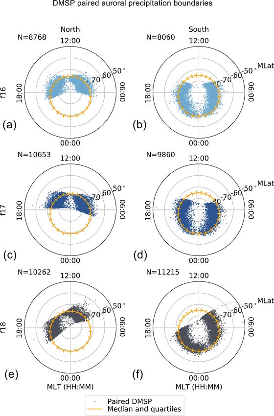
482                                                                                      A. G. Burrell et al.: AMPERE OCBs

cap. The physical processes that occur here are different from     OCB-oriented coordinates when studying the climatological
those that occur at other high-latitude regions where the mag-     behaviour of the plasma drift vorticity) when using adaptive,
netic field lines are closed (connect back to the Earth in the     high-latitude coordinates. Unfortunately, observations of the
opposite hemisphere). In the polar cap, magnetic field lines       OCB are sparse. Long-term and large-scale studies would
are moved from magnetic noon to magnetic midnight by the           benefit from specifications of the OCB in both hemispheres
solar wind, where they eventually reconnect with geomag-           and all magnetic local times (MLTs) every 15 min or less
netic field lines from the opposite hemisphere. Once closed,       (Cowley and Lockwood, 1992). Models that have the abil-
these field lines move to lower magnetic latitudes (the au-        ity to distinguish between regions with open and closed field
roral oval) and return towards the dayside. This process of        lines would also benefit from adaptive, high-latitude coordi-
reconnection is known as the Dungey cycle (Dungey, 1961),          nates (Zhu et al., 2019).
and (to first order) describes the motion of the magnetic field       This study presents a new set of OCBs obtained from the
lines and the ionospheric plasma frozen into those field lines.    Active Magnetosphere and Planetary Electrodynamics Re-
   At ionospheric altitudes, the open–closed field line bound-     sponse Experiment (AMPERE) magnetic perturbation obser-
ary (OCB) separates the polar cap from the auroral oval,           vations. AMPERE measurements of FACs make it possible
which is the highest latitude region to have closed magnetic       to estimate the location where Region 1 (R1) and Region 2
field lines. This boundary is important because the state of       (R2) FAC systems meet (the R1–R2 boundary). Because the
the field lines (open or closed) determines the types of cou-      location of the Birkeland current system is tied to the ex-
pling that may occur within the magnetosphere–ionosphere–          pansion and contraction of the polar cap under quiescent
thermosphere (MIT) system. One example of a difference in          and disturbed conditions (Coxon et al., 2018, and references
MIT coupling between the polar cap and auroral oval is field-      therein.), it seems logical to hypothesise that a dependable
aligned currents (FACs). The closed field lines in the auroral     relationship between the R1–R2 boundary and the OCB ex-
oval support the formation of current systems that link the        ists. This study investigates the relationship between the AM-
ionosphere to the magnetopause and current sheet (the Re-          PERE R1–R2 boundary and the OCB inferred from particle
gion 1 or R1 FAC system) and to the partial ring current in        precipitation measurements made by the Defense Meteoro-
the inner magnetosphere (the Region 2 or R2 FAC system)            logical Satellite Program Special Sensor J (DMSP SSJ) elec-
(Iijima and Potemra, 1976). Because the R1 FAC system con-         tron energy flux boundaries. This study has parallels with that
nects the ionosphere to the outer magnetosphere, it lies pole-     of Clausen et al. (2013), who compared the R1 peak loca-
ward of the R2 FAC system and moves with the OCB (Coxon            tion (as determined from a circle fitted to the R1 peaks at all
et al., 2018, and references therein).                             MLTs) with a range of different DMSP particle precipitation
   Another example of MIT coupling processes affected by           boundaries, showing a close relationship with the b5i and b5e
the OCB is the density structure of the high-latitude iono-        boundaries in the nightside ionosphere. Section 2 presents
sphere. Consider the unexceptional case of a southward IMF         the details of both data sets. Section 3 explores the rela-
and a partially illuminated high-latitude ionosphere. Under        tionship between the different boundaries and presents the
these conditions, ionospheric plasma follows a convective          calibration process that allows the AMPERE R1–R2 bound-
flow driven by the Dungey cycle, characterised by straight,        ary to be used as a proxy for the OCB. This calibration, as
anti-sunward plasma drifts within the polar cap and longer,        well as the previous Magnetopause-to-Aurora Global Explo-
curved, sunward drifts when the plasma are frozen into             ration (IMAGE) calibration performed by Chisham (2017b),
closed magnetic field lines (the boundary between these two        is validated in Sect. 4 by comparing calibrated OCBs with the
regions is commonly referred to as the convection rever-           CRBs from DMSP plasma drift measurements. CRBs were
sal boundary or CRB). The difference in convective mo-             chosen as a validation data set because the direction of con-
tion poleward and equatorward of the CRB creates a highly          vective plasma drifts are strongly tied to the motion and state
structured polar ionosphere, as the dense dayside ionospheric      (i.e. open or closed) of the magnetic field lines. This means
plasma is rapidly transported to the nightside where recombi-      that the CRB is typically located at or just equatorward of the
nation processes destroy plasma that does not return to sunlit     OCB (Newell et al., 2004; Drake et al., 2009), except for re-
regions quickly enough (due to having to follow the longer         gions of the dayside and nightside ionosphere that map to re-
return path through the auroral oval) (e.g. Spiro et al., 1978).   gions of ongoing magnetic reconnection. Finally, the results
   Due to these and other differences in MIT coupling pro-         of this study are summarised in Sect. 5.
cesses in the auroral oval and the polar cap, it is desirable to
have a coordinate system that indicates where (in which re-
gion) measurements were taken. This type of adaptive, high-        2   Instrumentation
latitude gridding has been performed with various data sets
(Redmon et al., 2010; Chisham, 2017b; Kilcommons et al.,           The data sets used in this study have a long and ongoing his-
2017). These studies have demonstrated improved statistical        tory of observations. The primary data set, AMPERE, is de-
and climatological results (for example, Chisham (2017b)           scribed in Sect. 2.1. Two instruments from DMSP are used,
demonstrated the difference between using magnetic and             one for calibration of the boundaries and another for valida-

Ann. Geophys., 38, 481–490, 2020                                                           www.ann-geophys.net/38/481/2020/
A. G. Burrell et al.: AMPERE OCBs                                                                                           483

tion. Both DMSP data sets are described in Sect. 2.2. The          2.2   DMSP
IMAGE far ultraviolet (FUV) data set used in the validation
is described in Sect. 2.3.                                         The DMSP OCB locations are obtained from energetic elec-
                                                                   tron fluxes measured by three DMSP spacecraft (F16–F18)
2.1   AMPERE                                                       that were operational and have updated ephemera (Red-
                                                                   mon et al., 2017) during the period of time when AM-
AMPERE assimilates measurements from the approximately             PERE R1–R2 boundaries were available. The DMSP satel-
70 polar-orbiting spacecraft of the Iridium telecommunica-         lites were located in sun-synchronous polar orbits at an al-
tions constellation to deduce the high-latitude distribution       titude of about 830 km, with an orbital period of approx-
of horizontal magnetic field perturbations produced by the         imately 101 min. The geographic locations of the DMSP
FACs responsible for magnetosphere–ionosphere coupling             SSJ/5 equatorward and poleward boundaries were deter-
(Anderson et al., 2000, 2002; Waters et al., 2001; Coxon           mined using ssj_auroral_boundary (Kilcommons and Bur-
et al., 2018). The FAC pattern in both hemispheres is cal-         rell, 2019), which implements the technique described in Kil-
culated from 10 min averages at a 2 min cadence on a mag-          commons et al. (2017). A clean set of OCBs were obtained
netic latitude and MLT grid (1◦ × 1 h resolution); this study      by selecting the poleward boundaries with figures of merit
employs R1–R2 FAC boundaries from 2010 to 2012 (Milan,             greater than 3.0 and calculating the AACGM-v2 coordinates
2019).                                                             at each location (Shepherd, 2014; Burrell et al., 2018b).
   The basis of the R1–R2 boundary identification is a fitting        The same DMSP spacecraft also carry an Ion Velocity Me-
technique described by Milan et al. (2015). This technique         ter (IVM) that measures the three-dimensional ion velocity
aims to determine the centre and radius of the circle that best    (Heelis and Hanson, 1998). As discussed in Sect. 1, the CRB
describes the boundary between the R1 and R2 FACs with-            is the location where plasma drifts change from moving sun-
out fitting to individual MLT bins. By avoiding this com-          ward to anti-sunward, or vice versa, and this boundary typ-
mon method of defining a high-latitude boundary, this R1–          ically lies at or just equatorward of the OCB (Newell et al.,
R2 boundary identification is more robust in the event of          2004; Drake et al., 2009).
sparse or weak currents and less influenced by the poorly             In this paper, CRBs obtained by Chen et al. (2015) are
defined current structures near local magnetic noon and mid-       used to validate the AMPERE OCB locations within an hour
night.                                                             of dawn (06:00 MLT) and dusk (18:00 MLT). Other MLTs
   The following procedure is applied to each AMPERE               were not considered for several reasons. Most importantly,
FAC grid. In this description, positive and negative values
represent upward and downward currents respectively. The            1. near magnetic noon and midnight the flows tend to be
R1 currents flow upwards at dusk and downwards at dawn,                mostly sunward or anti-sunward, meaning there is no
whereas the R2 currents have the opposite polarity and lie             clear reversal in the convection as a function of mag-
equatorward of the R1 current system. To distinguish be-               netic latitude;
tween these two FAC systems, the first step is to multiply all
FAC magnitudes on the dawn side (00:00 ≤ MLT < 12:00)               2. the IMF orientation will shift the MLT location of these
by −1. This redefines the current signs such that R1 FACs are          sunward or anti-sunward flows, meaning more local
positive and R2 FACs are negative at all MLTs. Then a centre           times than just noon and midnight are affected; and
point (x0 , y0 ) is assumed, where x0 is the dawnward distance
from the noon–midnight meridian and y0 is the sunward dis-          3. near midnight, the Harang reversal can give the appear-
tance from the dawn–dusk meridian. A range of centres are              ance of multiple convection reversals at different lati-
tested, with x0 varying between ± 4◦ and y0 varying between            tudes.
−6 and 0◦ latitude. Additionally, a range of radii are tested at      The Chen et al. (2015) algorithm is optimised to identify
each centre point; the radius is varied by 1◦ latitude (111 km)    the CRB in a two-cell convection pattern. If the plasma con-
from 8 to 35◦ . At each radius and centre point, the sum of the    vection has a complex pattern with more than four rever-
FACs at 200 equally spaced points in a ring centred at (x0 ,       sals, or the plasma flows are weak and noisy, the program
y0 ) is found. This produces a profile of integrated FAC mag-      will not identify any CRB location. For symmetric, multi-
nitude with the radius, in which a negative–positive bipolar       cell patterns (such as those observed when the IMF is domi-
signature is sought. The zero-crossing of the bipolar signa-       nated by a positive BZ component), the program will identify
ture is taken to be the R1–R2 boundary, and the peak-to-peak       the most equatorward reversal boundary. Otherwise, the most
magnitude provides a figure of merit (FOM) for the bound-          poleward reversal boundary will be selected as the CRB loca-
ary fit. For each AMPERE FAC grid, the circle with the best        tion. The algorithm typically performs better in the summer,
FOM is chosen, and grids with low FOMs are discarded as            as the DMSP IVM performs better when the plasma density
being unreliable.                                                  is higher (Chen et al., 2015; Chen and Heelis, 2018). These
                                                                   algorithmic biases mean that the CRBs cover May through
                                                                   August in the Northern Hemisphere and November through

www.ann-geophys.net/38/481/2020/                                                           Ann. Geophys., 38, 481–490, 2020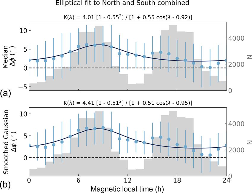
484 A. G. Burrell et al.: AMPERE OCBs
February in the Southern Hemisphere. However, even with on the AMPERE FAC maps (see Sect. 2.1). However, over
the difficulties introduced by nonsymmetric convection pat- 90 % of Northern Hemisphere pairs and over 80 % of South-
terns, all IMF clock angles are well represented in the CRB ern Hemisphere pairs have a temporal difference of 1 min or
data set. less. Good DMSP SSJ OCB detections are defined as having
a FOM of 3.0 or greater. This is consistent with the work pre-
2.3 IMAGE FUV sented by Kilcommons et al. (2017) and reduces the number
of passes with dayside precipitation associated with the cusp,
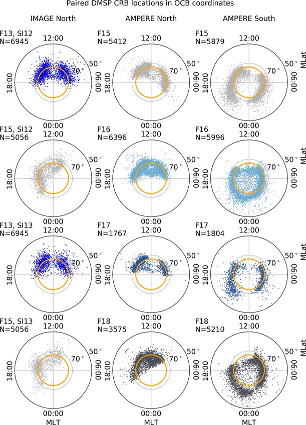
Chisham (2017b) obtained estimates of the OCB from auro- mantle, and other sources whose origin (inside or outside the
ral images measured by the FUV imagers onboard the IM- polar cap) is still debatable. The DMSP SSJ paired OCBs for
AGE spacecraft. Images of the Northern Hemisphere auroral each hemisphere and satellite are shown in Fig. 1 as a scat-
region were available for the epoch spanning from May 2000 ter plot, with the median location of the AMPERE R1–R2
to August 2002. During this time, the spacecraft was located boundaries plotted on top. Note that the R1–R2 boundaries
in an elliptical orbit with a 90◦ inclination, an apogee of 7 RE , lie near the equatorward edge of the DMSP SSJ OCBs. Be-
a perigee of 1000 km, and an orbital period of ∼ 13.5 h. cause of the DMSP satellite orbits, MLTs near noon are only
This study uses data from the two FUV spectrographic covered in the Northern Hemisphere and those near midnight
imagers, SI12 and SI13 (Mende et al., 2000). The SI13 im- are only covered in the Southern Hemisphere.
ager measured oxygen emissions at 135.6 nm, resulting from Ideally, observations from both hemispheres can be com-
energetic electron precipitation. The SI12 imager measured bined to provide complete MLT coverage of the differences
Doppler-shifted Lyman-α emissions at 121.8 nm, resulting between the AMPERE R1–R2 boundaries and DMSP SSJ
from proton precipitation. Both imagers provided data at OCBs. To test the assumption that the northern and south-
a 2 min resolution, when the Northern Hemisphere was vis- ern boundaries have the same local time dependence, the
ible. The OCB was identified in the individual FUV images MLT bins with observations in both hemispheres (05:00–
and fit across all magnetic local times using the techniques 08:00 and 15:00–20:00 MLT) were compared. The hourly
described by Longden et al. (2010) and Chisham (2017b). boundary offsets in each hemisphere and both hemispheres
combined, all calculated using the magnetic co-latitude, are
3 Relationship between the R1–R2 boundary and OCB presented in Table 1.
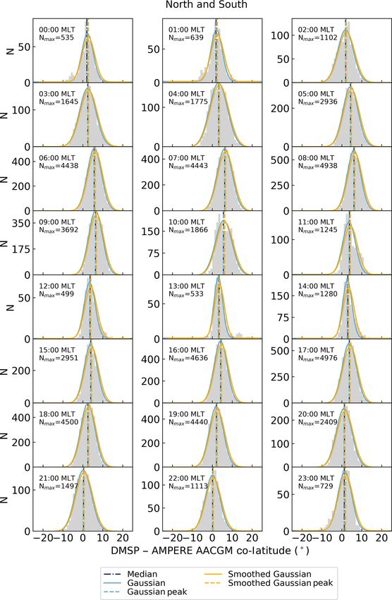
The boundary offsets in Table 1 were calculated by finding
This study follows the process outlined in Boakes et al. the typical difference between the DMSP SSJ OCB and the
(2008), which determined the offset between the IMAGE AMPERE R1–R2 boundary location in AACGM-v2 mag-
FUV poleward auroral boundaries and DMSP OCBs, to ob- netic latitude in 1 h MLT bins. The typical boundary lati-
tain a correction between the AMPERE R1–R2 boundary and tude difference (1φ, which equals the DMSP SSJ OCB co-
the DMSP SSJ OCBs. The five steps of this process are enu- latitude minus the AMPERE R1–R2 boundary co-latitude) is
merated in the following: represented by two values – the median of the boundary lati-
tude differences and the peak of a Gaussian distribution (S.G.
1. identify the AMPERE R1–R2 boundaries;
peak) – fitted to a smoothed histogram (as in Boakes et al.,
2. pair AMPERE R1–R2 boundaries with DMSP SSJ 2008). The histograms have 1◦ bins, and they were smoothed
OCBs; using a 4◦ running average. The smoothed histogram was
then fitted with a Gaussian function, allowing the S.G. peak
3. determine the typical offset at different MLTs;
and standard deviation to be calculated.
4. find a functional fit that describes the offset between Comparing the median and S.G. peak of the 1φ for the
the DMSP SSJ OCBs and the AMPERE R1–R2 bound- MLT bins with observations in both hemispheres shows
aries; and a mean hemispheric difference of −0.30 and 0.23◦ for the
median and S.G. peaks respectively. This difference is small
5. use the functional fit to correct the AMPERE R1–R2 enough to justify combining the northern and southern hemi-
boundary locations, creating an AMPERE OCB proxy. spheric 1φ, as it is much smaller than the mean standard de-
This study uses AMPERE R1–R2 boundaries, described in viation of the MLT distributions (σ = 2.66◦ for the overlap-
Sect. 2.1, from January 2010 through December 2012. Us- ping MLT bins). The results for the combined hemispheres
ing only R1–R2 boundaries with FOMs greater than 0.15 mA are presented in the rightmost columns of Table 1 and in
provides 636 250 Northern Hemisphere and 531 666 South- Fig. 2. There is about a 0.49◦ difference between the median
ern Hemisphere boundary locations. Pairing these bound- and S.G. peak values. This difference is very small compared
aries to good DMSP SSJ OCB detections by requiring each with the width of the 1φ distributions, and it provides a mea-
observation be taken within 10 min of each other leaves sure of uncertainty for the resulting boundary correction.
29 683 Northern Hemisphere and 29 135 Southern Hemi- Unfortunately, the differences between the boundary fit-
sphere boundaries. The 10 min window for pairing bound- ting methodology used by Chisham (2017b) and Milan et al.
aries was chosen because of the 10 min averaging performed (2015) mean that it is not reasonable to use a harmonic func-
Ann. Geophys., 38, 481–490, 2020 www.ann-geophys.net/38/481/2020/A. G. Burrell et al.: AMPERE OCBs 485
Table 1. Hourly boundary offset for hours with over 100 boundary pairs and successfully fit Gaussians.
MLT North South Both
Median (◦ ) S.G. peak (◦ ) Median (◦ ) S.G. peak (◦ ) Median (◦ ) S.G. peak (◦ )
00:00 – – 2.04 2.83 2.04 2.83
01:00 – – 1.88 2.56 1.88 2.56
02:00 – – 1.93 2.36 1.93 2.36
03:00 – – 2.46 2.94 2.46 2.94
04:00 – – 3.20 3.60 3.20 3.60
05:00 3.96 4.45 4.80 5.29 4.33 4.86
06:00 5.16 5.69 6.34 – 5.73 6.26
07:00 5.29 5.88 6.98 – 6.21 6.71
08:00 5.69 6.19 7.10 – 6.08 6.64
09:00 5.38 5.99 – – 6.35 6.88
10:00 4.64 5.29 – – 5.64 6.23
11:00 3.78 4.27 – – 3.82 4.32
12:00 3.57 3.99 – – 3.66 4.04
13:00 3.30 3.61 – – 3.40 3.62
14:00 2.95 3.36 – – 3.02 3.43
15:00 3.49 3.97 5.21 5.76 3.97 4.50
16:00 4.20 4.68 4.19 4.66 4.19 4.67
17:00 4.00 4.47 3.32 3.74 3.77 4.22
18:00 2.82 3.30 2.27 2.77 2.54 3.01
19:00 2.67 3.12 1.52 1.95 2.07 2.51
20:00 2.42 3.13 0.96 1.35 1.29 1.63
21:00 – – 0.33 0.73 0.33 0.73
22:00 – – 0.14 0.60 0.14 0.60
23:00 – – 1.24 1.94 1.24 1.94
Table 2. Boundary fit constants for DMSP − AMPERE boundary τ is the angular offset of the ellipse’s centre in radians. These
offset. four constants allow the ellipse to adjust its centre and axes.
They are fit using the Python SciPy least squares fitting rou-
Constant Median S.G. peak tine, leastsq (Virtanen et al., 2020), which wraps the MIN-
a 4.01◦ 4.41◦ PACK LMDIF and LMDER algorithms (More et al., 1984).
e 0.55 0.51 The least squares fitting routine minimises the difference be-
τ −0.92 −0.95 tween K and 1φ, weighted by the inverse of the error, .
The error is defined as shown in Eq. (2), where NMLT is the
number of 1φ observations in each MLT bin, Nmax is the
tion to describe the offset between the DMSP SSJ OCBs and maximum NMLT , and σ is either the interquartile range or
the AMPERE R1–R2 boundaries, as done in prior auroral the standard deviation depending on whether the median or
boundary fitting studies (Holzworth and Meng, 1975; Car- S.G. peak was used as the central value. The results of this
bary et al., 2003; Boakes et al., 2008). Because the R1–R2 fitting procedure are shown in Fig. 3 and Table 2.
boundary fitting method used by Milan et al. (2015) does
s
NMLT 2
not fit a series of MLT bins, the boundary correction cannot = +σ2 (2)
be applied prior to circle fitting and will determine the final Nmax
shape of the OCB proxy. Thus, this study uses a generalised
ellipse (Eq. 1) rather than a harmonic function to avoid over- As shown in Fig. 3, the AMPERE R1–R2 boundary lies
fitting the MLT dependence of the offset between the DMSP about 2◦ equatorward of the OCB at magnetic midnight,
SSJ OCBs and the AMPERE R1–R2 boundaries. about 4◦ equatorward of the OCB at magnetic noon, and
further out at dawn and dusk. The elliptical fit follows the
a(1 − e2 ) central values very closely between 00:00 and 10:00 MLT,
K(λ) = (1) and it smooths through the maxima and minima at 12:00,
1 + e cos(λ − τ )
16:00, and 22:00 MLT. However, even where the differences
In Eq. (1), λ is the MLT in radians, a is the semi-major are greatest, the elliptical fit does not differ from the central
axis in degrees, e is the eccentricity (a unitless quantity), and value by more than /2. This behaviour is consistent whether
www.ann-geophys.net/38/481/2020/ Ann. Geophys., 38, 481–490, 2020486 A. G. Burrell et al.: AMPERE OCBs Figure 1. Paired AMPERE R1–R2 boundaries and DMSP SSJ Figure 2. Hourly distributions of paired AMPERE R1–R2 bound- OCBs for both hemispheres (Northern Hemisphere is shown in a, c, ary and DMSP SSJ OCB latitude differences, with boundary differ- and e; Southern Hemisphere is shown in, b, d, and f) and each satel- ences from both hemispheres and all satellites. The black dashed lite. The scattered points show the DMSP SSJ OCBs, and the gold line shows the median of the distribution, the blue line shows circle shows the median location of the AMPERE R1–R2 bound- a Gaussian fit to the distribution and the gold line shows the Gaus- aries. The scatter bars denote the quartiles of the paired AMPERE sian fit to the smoothed histogram. The vertical blue and gold lines R1–R2 boundaries. show the peaks of each Gaussian fit. the median or S.G. peak is used in the fitting process. The 4 Validation similarity between the two fits can be quantified by compar- ing the differences between aMedian and aS.G. Peak (0.40◦ ) and The appropriateness of using K to transform the AMPERE the typical difference between the hourly median and S.G. R1–R2 boundary into an AMPERE OCB is tested by com- peak values (0.49◦ ); the differences between the eccentricity paring the AMPERE OCBs to the DMSP CRBs within an and angular offset are even less significant. hour of dawn and dusk. These local times were chosen due The consistency of the elliptical fit for both central val- to the MLT-dependent variations in the CRB–OCB relation- ues, as well as its success at capturing the major features of ship discussed in Sect. 2.2. It should also be reiterated that 1φ given the functional constraints, make it a good candi- no specific selection was made for IMF conditions. All IMF date for correcting the R1–R2 boundary to provide an OCB clock angles and magnitudes are considered together, as the estimate. The Gaussian nature of the hourly bins (shown in AMPERE OCBs should be valid at all IMF conditions when Fig. 2) suggests that differences between the R1–R2 bound- the OCB can be represented (to first order) by an ellipse. To ary and DMSP SSJ OCB are randomly distributed, confirm- ensure that the performance of the AMPERE OCBs are on ing the conclusion that it is appropriate to use K to correct par with previous OCB calculations, this validation is also the R1–R2 boundary to obtain an AMPERE OCB estimate. performed for the IMAGE OCBs. Unfortunately, it is impos- Ann. Geophys., 38, 481–490, 2020 www.ann-geophys.net/38/481/2020/
A. G. Burrell et al.: AMPERE OCBs                                                                                                     487

Figure 3. Elliptical boundary correction (black line) fit to the me-
dian (a) and S.G. peak (b) 1φ for both hemispheres. The blue dots
and scatter bars show the central value and  in each MLT bin re-
spectively. The grey histogram shows NMLT , and scales to the y axis
on the right.

sible to directly compare the AMPERE and IMAGE OCBs
because there is no temporal overlap between the two data
sets. This validation effort paired OCBs with DMSP CRBs
that were identified within 10 min of one another. The loca-
tion of the DMSP CRB relative to the OCB was then deter-
mined. In this adaptive coordinate system, the OCB is set at           Figure 4. Paired IMAGE and AMPERE OCBs with DMSP CRBs
a co-latitude of 74◦ (a latitude chosen to represent the OCB in        for the available hemispheres and each satellite. The IMAGE data
adaptive, high-latitude coordinates based on the typical size          show the SI12 and SI13 observations for the Northern Hemisphere
of the polar cap). CRBs that occur poleward or equatorward             (left column), while the median elliptical correction was applied to
of the OCB will have co-latitudes greater than or less than            obtain the AMPERE OCBs shown in the middle and right columns
74◦ respectively. This adaptive gridding was performed us-             (which show the Northern Hemisphere and Southern Hemisphere
ing the ocbpy Python package (Burrell and Chisham, 2018;               respectively). The scattered points show the DMSP IVM CRBs, and
Burrell et al., 2018a).                                                the gold circle shows the IMAGE or AMPERE OCB. To simplify
   Figure 4 shows the distribution of CRB observations                 the comparison, the DMSP IVM CRB locations are plotted in ad-
                                                                       justed polar coordinates (Burrell and Chisham, 2018). Although all
for the different DMSP satellites, OCB sources, and hemi-
                                                                       CRBs paired with IMAGE or AMPERE OCBs are shown here, only
spheres. As was done with the DMSP SSJ observations,
                                                                       CRBs within 1 h of 06:00 or 18:00 MLT were used in this validation.
2 years of CRBs and OCBs were paired in time after re-
moving unreliable boundaries (as discussed in Sect. 2). Note
that the paired data, both from the two IMAGE instruments              of the distributions is below 5◦ in all places. Additionally, the
and from AMPERE (in both hemispheres), show a similar                  CRB is approximately co-located with both the AMPERE
spread of CRBs at different magnetic local times, with larger          and IMAGE OCBs. This close agreement with the DMSP
spreads near magnetic noon and midnight.                               CRB and the similar behaviour of the IMAGE and AMPERE
   Figure 5 shows the histograms of the latitude differences           OCBs validates the AMPERE OCBs provided here.
between the DMSP CRBs and the IMAGE (Fig. 5a, d) or
AMPERE (Fig. 5b, c, e, f) OCBs. This figure also shows the
results for the median ellipse correction to obtain the AM-            5   Conclusions
PERE OCB (Fig. 5a, b, c) and the S.G. peak ellipse correc-
tion (Fig. d, e, f). For the IMAGE histograms, Fig. 5a shows           This study modified traditional auroral boundary fitting
the results for the SI13 instrument, and Fig. 5d shows the re-         methods to establish an MLT-dependent relationship between
sults for the SI12 instrument. In all cases, the means and me-         the OCB and the R1–R2 boundary. This was performed by
dians of the difference distributions behave similarly: most           determining the first moment of the distribution of differ-
points lie within 1◦ of each other, and the standard deviation         ences between the R1–R2 boundary and the OCB (as mea-

www.ann-geophys.net/38/481/2020/                                                                  Ann. Geophys., 38, 481–490, 2020
488 A. G. Burrell et al.: AMPERE OCBs
Figure 5. Histograms showing the differences between DMSP CRB and IMAGE or AMPERE OCB using paired boundaries that occur
within 1 h of 06:00 or 18:00 MLT.
sured by the DMSP SSJ instrument) for 1 h MLT bins. These We thank the PI, the IMAGE mission, and the IMAGE FUV
moments (which included the median of the distribution and team for data usage and processing tools. The raw IMAGE data
the peak of a smoothed Gaussian fit) were then used to define and software are available from http://sprg.ssl.berkeley.edu/image/
the parameters of an elliptical function. This function speci- (Frey, 2017). The auroral boundary data set and the methodology
fies the distance between the OCB and R1–R2 boundary as used to create it can be found at https://www.bas.ac.uk/project/
image-auroral-boundary-data/ (last access: August 2019) or in
a function of MLT.
Chisham (2017a).
The validity of this OCB, as well as previously determined DMSP data are available at http://cedar.openmadrigal.org (Ride-
IMAGE OCBs, were tested against the dawn and dusk mea- out, 2019), and https://cdaweb.gsfc.nasa.gov (Kovalick, 2019).
surements of the CRB (as measured by several DMSP IVM DMSP SSJ boundaries may be obtained using the software avail-
instruments). These boundaries were found to typically differ able at https://doi.org/10.5281/zenodo.3267415 (Kilcommons and
by less than a degree. Burrell, 2019) and https://doi.org/10.5281/zenodo.3373812 (Kil-
As mentioned in the introduction, modelling and statisti- commons et al., 2019). DMSP CRBs can be requested from Yun-
cal studies in polar regions should avoid mixing measure- Ju Chen (yxc126130@utdallas.edu).
ments taken in the auroral oval and the polar cap. In combi- The software that was used to perform adaptive, high-latitude
nation, the AMPERE and IMAGE OCBs form the basis of gridding can be found at https://github.com/aburrell/ocbpy (last
a multi-solar cycle data set that could be used to improve access: August 2019) or https://doi.org/10.5281/zenodo.1217177
(Burrell and Chisham, 2018).
high-latitude statistical studies and climatological models.
The data sets and software tools presented in this paper allow
researchers to begin using adaptive, high-latitude coordinates
Author contributions. AGB developed the concept, performed the
in their investigations.
data analysis, and wrote the paper. GC supported the conceptual de-
velopment, provided feedback on the data analysis, and edited the
paper. SEM provided the AMPERE R1–R2 boundaries and guide-
Code and data availability. AMPERE data are available from the lines for their use, provided feedback on the conceptual develop-
John Hopkins University Applied Physics Laboratory at http:// ment, and contributed to writing the paper. LK provided guidelines
ampere.jhuapl.edu/ (John Hopkins Applied Physics Laboratory, for the use of the DMSP SSJ boundaries, gave feedback on the val-
2019). We thank the AMPERE team and the AMPERE Science idation, and edited the paper. YJC provided the DMSP CRBs, sup-
Center for providing the Iridium-derived data products. AMPERE plied guidelines for their use in validation, and edited the paper.
boundaries are described in Milan et al. (2015) and can be ac- EGT provided feedback on the data validation efforts and edited the
cessed at https://doi.org/10.25392/leicester.data.11294861.v1 (Mi- paper. BA is the PI of AMPERE.
lan, 2019) or through ocbpy (Burrell and Chisham, 2018).
The IMAGE FUV data are provided courtesy of the instru-
ment PI Stephen Mende (University of California, Berkeley).
Ann. Geophys., 38, 481–490, 2020 www.ann-geophys.net/38/481/2020/A. G. Burrell et al.: AMPERE OCBs 489
Competing interests. The authors declare that they have no conflict Chen, Y.-J. and Heelis, R. A.: Motions of the Convec-
of interest. tion Reversal Boundary and Local Plasma in the High-
Latitude Ionosphere, J. Geophys. Res.-Space, 123, 2953–2963,
https://doi.org/10.1002/2017ja024934, 2018.
Acknowledgements. Angeline G. Burrell is supported by the United Chen, Y.-J., Heelis, R. A., and Cumnock, J. A.: Response of the
States Chief of Naval Research (US CNR). Gareth Chisham is sup- ionospheric convection reversal boundary at high latitudes to
ported by United Kingdom Research and Innovation (UKRI) as part changes in the interplanetary magnetic field, J. Geophys. Res.-
of the British Antarctic Survey – Polar Science for Planet Earth Space, 120, 5022–5034, https://doi.org/10.1002/2015ja021024,
Programme. Liam Kilcommons is supported by AFOSR (award 2015.
no. FA9550-17-1-0258). Yun-Ju Chen is supported by an AFOSR Chisham, G.: Auroral Boundary Derived from IMAGE Satel-
MURI grant (grant no. FA9559-16-1-0364) to The University of lite Mission Data (May 2000–Oct 2002), British Antarc-
Texas at Dallas. Evan G. Thomas is supported by a NSF grant. The tic Survey, https://doi.org/10.5285/75aa66c1-47b4-4344-ab5d-
authors would like to thank Jone Peter Reistad for communications 52ff2913a61e, 2017a.
about the “Discussion Paper” version of this paper that lead to im- Chisham, G.: A new methodology for the development
portant improvements. of high-latitude ionospheric climatologies and empir-
ical models, J. Geophys. Res.-Space, 122, 932–947,
https://doi.org/10.1002/2016JA023235, 2017b.
Financial support. This research has been supported by the United Clausen, L. B. N., Baker, J. B. H., Ruohoniemi, J. M., Milan, S. E.,
States Chief of Naval Research (US CNR); the United Kingdom Coxon, J. C., Wing, S., Ohtani, S., and Anderson, B. J.: Tem-
Research and Innovation (UKRI), British Antarctic Survey – Po- poral and spatial dynamics of the regions 1 and 2 Birkeland
lar Science for Planet Earth Programme; the Air Force Office of currents during substorms, J. Geophys. Res.-Space, 118, 3007–
Scientific Research (grant nos. FA9550-17-1-0258 and FA9559-16- 3016, https://doi.org/10.1002/jgra.50288, 2013.
1-0364); and the National Science Foundation, Office of Polar Pro- Cowley, S. W. H. and Lockwood, M.: Excitation and decay of
grams (grant no. OPP-1836426). solar-wind driven flows in the magnetosphere-ionosphere sys-
tem, Ann. Geophys., 10, 103–115, 1992.
Coxon, J. C., Milan, S. E., and Anderson, B. J.: A review of Birke-
land current research using AMPERE, vol. 235, chap., in: Elec-
Review statement. This paper was edited by Keisuke Hosokawa
tric Currents in Geospace and Beyond, American Geophysical
and reviewed by two anonymous referees.
Union, https://doi.org/10.1002/9781119324522.ch16, 257–278,
2018.
Drake, K. A., Heelis, R. A., Hairston, M. R., and Anderson, P. C.:
Electrostatic Potential Drop Across the Ionospheric Signature
References of the Low-Latitude Boundary Layer, J. Geophys. Res., 114,
A04215, https://doi.org/10.1029/2008JA013608, 2009.
Anderson, B. J., Takahashi, K., and Toth, B. A.: Sensing global Dungey, J. W.: Interplanetary Magnetic Field and the Auroral
Birkeland currents with Iridium engineering magnetometer data, Zones, Phys. Rev. Lett., 6, 47–48, 1961.
Geophys. Res. Lett., 27, 4045–4048, 2000. Frey, H. U.: Image, available at: http://sprg.ssl.berkeley.edu/image/,
Anderson, B. J., Takahashi, K., Kamei, T., Waters, C. L., last access: August 2017.
and Toth, B. A.: Birkeland current system key param- Heelis, R. A. and Hanson, W. B.: Measurements of Thermal Ion
eters derived from Iridium observations: Method and Drift Velocity and Temperature using Planar Sensors, in: Mea-
initial validation results, J. Geophys. Res., 107, 1079, surement Techniques in Space Plasmas: Particles, edited by:
https://doi.org/10.1029/2001JA000080, 2002. Pfaff, R. F., Borovsky, J., and Young, T. D., AGU, Washington,
Boakes, P. D., Milan, S. E., Abel, G. A., Freeman, M. P., Chisham, D.C., https://doi.org/10.1029/GM102, 61–71, 1998.
G., Hubert, B., and Sotirelis, T.: On the use of IMAGE FUV Holzworth, R. and Meng, C.-I.: Mathematical Representation of the
for estimating the latitude of the open/closed magnetic field line Auroral Oval, Geophys. Res. Lett., 2, 377–380, 1975.
boundary in the ionosphere, Ann. Geophys., 26, 2759–2769, Iijima, T. and Potemra, T. A.: The Amplitude Distribution of Field-
https://doi.org/10.5194/angeo-26-2759-2008, 2008. Aligned Currents at Northern High Latitudes Observed by Triad,
Burrell, A. G. and Chisham, G.: aburrell/ocbpy: Beta Release, Zen- J. Geophys. Res., 81, 2165–2174, 1976.
odo, https://doi.org/10.5281/zenodo.1217177, 2018. John Hopkins Applied Physics Laboratory: AMPERE, available at:
Burrell, A. G., Halford, A., Klenzing, J., Stoneback, R. A., Mor- http://ampere.jhuapl.edu/, last access: August 2019.
ley, S. K., Annex, A. M., Laundal, K. M., Kellerman, A. C., Kilcommons, L. and Burrell, A. G.: lkilcom-
Stansby, D., and Ma, J.: Snakes on a Spaceship—An Overview mons/ssj_auroral_boundary: Version 1 (Version v1.0.0),
of Python in Heliophysics, J. Geophys. Res.-Space, 123, 10384– Zenodo, https://doi.org/10.5281/zenodo.3267415, 2019.
10402, https://doi.org/10.1029/2018ja025877, 2018a. Kilcommons, L. M., Redmon, R. J., and Knipp, D. J.: A new
Burrell, A. G., van der Meeren, C., and Laundal, DMSP magnetometer and auroral boundary data set and es-
K. M.: aburrell/aacgmv2: AACGMV2 2.5.1, Zenodo, timates of field-aligned currents in dynamic auroral bound-
https://doi.org/10.5281/zenodo.1469697, 2018b. ary coordinates, J. Geophys. Res.-Space, 122, 9068–9079,
Carbary, J. F., Sotirelis, T., Newell, P. T., and Meng, C.-I.: Auro- https://doi.org/10.1002/2016ja023342, 2017.
ral boundary correlations between UVI and DMSP, J. Geophys.
Res., 108, 1018, https://doi.org/10.1029/2002JA009378, 2003.
www.ann-geophys.net/38/481/2020/ Ann. Geophys., 38, 481–490, 2020490 A. G. Burrell et al.: AMPERE OCBs Kilcommons, L., Redmon, R., and Knipp, D.: Defense Meteorol- Redmon, R. J., Denig, W. F., Kilcommons, L. M., and Knipp, ogy Satellite Program (DMSP) Electron Precipitation (SSJ) Au- D. J.: New DMSP database of precipitating auroral elec- roral Boundaries, 2010–2014 (Version 1.0.0) [Data set], Zenodo, trons and ions, J. Geophys. Res.-Space, 122, 9056–9067, https://doi.org/10.5281/zenodo.3373812, 2019. https://doi.org/10.1002/2016JA023339, 2017. Kovalick, T.: SPDF – Coordinated Data Analysis Web (CDAWeb), Rideout, B.: Madrigal database at CEDAR, available at: http://cedar. available at: https://cdaweb.gsfc.nasa.gov, last access: Au- openmadrigal.org, last access: August 2019. gust 2019. Shepherd, S. G.: Altitude-adjusted corrected geomag- Longden, N., Chisham, G., Freeman, M. P., Abel, G. A., and netic coordinates: Definition and functional approx- Sotirelis, T.: Estimating the location of the open-closed magnetic imations, J. Geophys. Res.-Space, 119, 7501–7521, field line boundary from auroral images, Ann. Geophys., 28, https://doi.org/10.1002/2014JA020264, 2014. 1659–1678, https://doi.org/10.5194/angeo-28-1659-2010, 2010. Spiro, R. W., Heelis, R. A., and Hanson, W. B.: Ion Convection and Mende, S. B., Heetderks, H., Frey, H. U., Stock, J. M., Lampton, the Formation and of the Mid-Latitude and F Region Ionization M., Geller, S. P., Abiad, R., Siegmund, O. H. W., Habraken, Trough, J. Geophys. Res., 83, 4255–4254, 1978. S., Renotte, E., Jamar, C., Rochus, P., Gérard, J. C., Sigler, R., Virtanen, P., Gommers, R., Oliphant, T. E., Haberland, M., Reddy, and Lauche, H.: Far ultraviolet imaging from the IMAGE space- T., Cournapeau, D., Burovski, E., Peterson, P., Weckesser, W., craft. 3. Spectral imaging of Lyman-alpha and OI 135.6 nm, Bright, J., van der Walt, S. J., Brett, M., Wilson, J., Millman, K. Space Sci. Rev., 91, 287–381, https://doi.org/10.1007/978-94- J., Mayorov, N., Nelson, A. R. J., Jones, E., Kern, R., Larson, 011-4233-5_10, 2000. R., Carey, C. J., Polat, İ., Feng, Y., Moore, E. W., VanderPlas, J., Milan, S.: AMPERE R1/R2 FAC radii, University of Leicester, Laxalde, D., Perktold, J., Cimrman, R., Henriksen, I., Quintero, https://doi.org/10.25392/leicester.data.11294861.v1, 2019. E. A., Harris, C. R., Archibald, A. M., Ribeiro, A. H., Pedregosa, Milan, S. E., Carter, J. A., Korth, H., and Anderson, B. J.: Prin- F., van Mulbregt, P., and SciPy 1.0 Contributors: SciPy 1.0: Fun- cipal component analysis of Birkeland currents determined by damental Algorithms for Scientific Computing in Python, Nat. the Active Magnetosphere and Planetary Electrodynamics Re- Methods, in press, 2020. sponse Experiment, J. Geophys. Res.-Space, 120, 10415–10424, Waters, C. L., Anderson, B. J., and Liou, K.: Estimation of Global https://doi.org/10.1002/grl.50505, 2015. and Field Aligned Currents Using the Iridium System Magne- More, J., Sorenson, D., Garbow, B., and Hillstrom, K.: The MIN- tometer Data, Geophys. Res. Lett., 28, 2165–2168, 2001. PACK Project, in: Sources and Development of Mathemati- Zhu, Q., Deng, Y., Richmond, A., Maute, A., Chen, Y.- cal Software, edited by: Cowell, W., Prentice-Hall, Englewood J., Hairston, M., Kilcommons, L., Knipp, D., Redmon, R., Cliffs, NJ, USA, available at: https://www.netlib.org/minpack/ and Mitchell, E.: Impacts of binning methods on high- (last access: August 2019), 1984. latitude electrodynamic forcing: static vs. boundary-oriented bin- Newell, P. T., Ruohoniemi, J. M., and Meng, C.-I.: Maps of ning methods, J. Geophys. Res.-Space, 124, e2019JA027270, precipitation by source region, binned by IMF, with iner- https://doi.org/10.1029/2019JA027270, 2019. tial convection streamlines, J. Geophys. Res., 109, A10206, https://doi.org/10.1029/2004JA010499, 2004. Redmon, R. J., Peterson, W. K., Andersson, L., Kihn, E. a., Denig, W. F., Hairston, M., and Coley, R.: Vertical thermal O+ flows at 850 km in dynamic auroral boundary coordinates, J. Geo- phys. Res., 115, A00J08, https://doi.org/10.1029/2010JA015589, 2010. Ann. Geophys., 38, 481–490, 2020 www.ann-geophys.net/38/481/2020/
You can also read