Monte Carlo Tree Search in Continuous Spaces Using Voronoi Optimistic Optimization with Regret Bounds
←
→
Page content transcription
If your browser does not render page correctly, please read the page content below
The Thirty-Fourth AAAI Conference on Artificial Intelligence (AAAI-20)

                        Monte Carlo Tree Search in Continuous Spaces
                  Using Voronoi Optimistic Optimization with Regret Bounds
   Beomjoon Kim,1 Kyungjae Lee,2 Sungbin Lim,3 Leslie Pack Kaelbling,1 Tomás Lozano-Pérez1
                                  1
                                      MIT Computer Science and Artificial Intelligence Laboratory
                                                  {beomjoon, lpk, tlp}@mit.edu
                                                    2
                                                      Seoul National University
                                                  kyungjae.lee@cpslab.snu.ac.kr
                                                           3
                                                             Kakao Brain
                                                  sungbin.lim@kakaobrain.com

                           Abstract
  Many important applications, including robotics, data-center
  management, and process control, require planning action se-
  quences in domains with continuous state and action spaces
  and discontinuous objective functions. Monte Carlo tree
  search (MCTS) is an effective strategy for planning in dis-
  crete action spaces. We provide a novel MCTS algorithm
  (VOOT) for deterministic environments with continuous ac-
  tion spaces, which, in turn, is based on a novel black-box
  function-optimization algorithm (VOO) to efficiently sam-
  ple actions. The VOO algorithm uses Voronoi partitioning                  Figure 1: Packing domain: the task is to pack as many
  to guide sampling, and is particularly efficient in high-                  objects coming from a conveyor belt into the room (left).
  dimensional spaces. The VOOT algorithm has an instance of                 Object-clearing domain: obstacles must be cleared from the
  VOO at each node in the tree. We provide regret bounds for
  both algorithms and demonstrate their empirical effectiveness
                                                                            swept-volume of a path to the sink (right). In both domains,
  in several high-dimensional problems including two difficult               the robot needs to minimize the overall trajectory length.
  robotics planning problems.

                                                                               Recently, several gradient-free approaches to continuous-
                       Introduction                                         space planning problems have been proposed (Buşoniu et
We are interested in finite-horizon deterministic planning                   al. 2011; Munos 2014; Weinstein and Littman 2012; Mans-
problems with high-dimensional continuous action spaces,                    ley, Weinstein, and Littman 2011), some of which have
with possibly a discontinuous objective function. For exam-                 been proven to asymptotically find a globally optimal so-
ple, consider the sequential robot mobile-manipulation plan-                lution. These approaches either frame the problem as si-
ning problem shown in Figure 1 (left). In this domain, the                  multaneously optimizing a whole action sequence (Buşoniu
objective function is defined to be the number of objects that               et al. 2011; Weinstein and Littman 2012) or treat the ac-
the robot packs into the storage room while satisfying fea-                 tion space in each node of a tree search (Mansley, We-
sibility conditions, such as collision-free motions, and min-               instein, and Littman 2011) as the search space for a
imizing the total length of its trajectory. Another example is              budgeted-black-box function optimization (BBFO) algo-
shown in Figure 1 (right), where the task is to clear obstacles             rithm, and use hierarchical-partitioning-based optimization
from a region, and the objective is a function of the number                algorithms (Munos 2011; Bubeck et al. 2011) to approxi-
of obstacles cleared and trajectory length. In both cases, the              mately find the globally optimal solution.
robot’s action space is high dimensional, consisting of mul-                   While these hierarchical-partitioning algorithms handle
tiple pick or placement configurations of the robot.                         a richer class of objective functions than traditional meth-
   More generally, such discontinuous objective functions                   ods (Pintér 1996), their main drawback is poor scalabil-
are the sum of a finite set of step functions in a high-                     ity to high-dimensional search spaces: to optimize effi-
dimensional state-action space, where each step corresponds                 ciently, these algorithms sequentially construct partitions of
to the occurrence of an important event, such as placing                    the search space where, at each iteration, they create a finer-
an object. For classes of functions of this kind, standard                  resolution partition inside the most promising cell of the
gradient-based optimization techniques are not directly ap-                 current partition. The problem is that constructing a parti-
plicable, and even if we smooth the objective function, the                 tion requires deciding the optimal dimension to cut, which
solution is prone to local optima.                                          is a difficult combinatorial problem especially in a high-
Copyright  c 2020, Association for the Advancement of Artificial            dimensional space. Figure 2 (left) illustrates this issue with
Intelligence (www.aaai.org). All rights reserved.                           one of the algorithms, DOO (Munos 2011).

                                                                     9916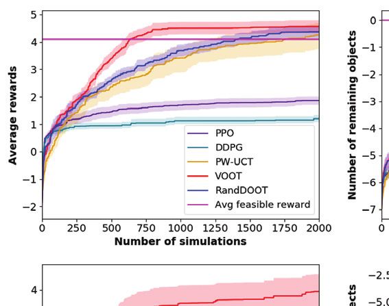
We propose a new BBFO algorithm called Voronoi Op-
timistic Optimization (VOO) which, unlike the previous ap-
proaches, only implicitly constructs partitions, and so scales
to high-dimensional search spaces more effectively. Specifi-
cally, partitions in VOO are Voronoi partitions whose cells
are implicitly defined as the set of all the points that are
closer to the generator than to any other evaluated point. Fig-
ure 2 (right) shows an example.
   Given as inputs a semi-metric, a bounded search space,                Figure 2: Left: Illustrations of a partition made by DOO when
and an exploration probability ω, VOO operates similarly                 five points are evaluated to optimize a 2D Shekel function.
to the previous partition-based methods: at each iteration,              Each solid line shows the partitions made by the point that is
it selects (implicitly) a Voronoi cell based on a simple                 on it. Numbers indicate the order of evaluations. The dotted
exploration-exploitation scheme, samples a point from the                lines indicate the two possible partitions that can be made
cell, and (implicitly) makes finer-resolution cells inside the            by the fifth point, and depending on this choice, the per-
selected cell based on the sampled point. The selection of               formance differs. Right: Illustration of the Voronoi parti-
a Voronoi cell is based on the given exploration probability:            tion implicitly constructed by VOO. We can sample from the
with probability ω, it explores by selecting a cell with proba-          best Voronoi cell (defined by the black point) by random-
bility proportional to the volume of the cell; with probability          sampling points, and rejecting them until we obtain one that
1 − ω, it exploits by selecting the cell that contains the cur-          is closer to the black point than the other points. We can sam-
rent best point. Unlike the previous methods, however, VOO               ple a point with Voronoi bias by uniformly sampling from
never explicitly constructs the partitions: by using the defi-            the entire search space; the cell defined by the white point is
nition of Voronoi partition and the given semi-metric, sam-              most likely to be selected.
pling from the best cell is implemented simply using rejec-
tion sampling. Sampling a point based on the volumes of
the cells, which is also known as the Voronoi bias (Kuffner
and LaValle 2000), is also simply implemented by sampling
                                                                                               Related work
uniformly at random from the search space. Figure 2 (right)              There are several planning methods that use black-box func-
demonstrates this point. We prove the regret bound of VOO                tion optimization algorithms in continuous-space problems.
which shows that under some mild assumptions, the regret                 We first give an overview of the BBFO algorithms, and then
goes to zero.                                                            describe planning algorithms that use them. We then give
   Using VOO, we propose a novel continuous state-action-                an overview of progressive-widening approaches, which are
space Monte Carlo tree search (MCTS) algorithm, Voronoi                  continuous-space MCTS algorithms that do not use black-
optimistic optimization applied to trees (VOOT) that uses                box function optimization methods.
VOO at each node of the search tree to select the optimal ac-            Global optimization of black-box functions with budget
tion, in a similar fashion to HOOT (Mansley, Weinstein, and                 Several partition-based algorithms have been pro-
Littman 2011). HOOT, however, does not come with per-                    posed (Munos 2011; Bubeck et al. 2011; Munos 2014). In
formance guarantees; we are able to prove a performance                  (Munos 2011), two algorithms are proposed. The first algo-
guarantee for VOOT, which is derived from a bound on the                 rithm is DOO, which requires as inputs a semi-metric and the
regret of VOO. The key challenge in showing this result is               Lipschitz constant for the objective function. It sequentially
that, when VOO is used to optimize the state-action value                constructs partitions of the search space, where a cell in the
function of a node in the tree, the value function is non-               partition has a representative point, on which the objective
stationary, so that even when the environment is determinis-             function is evaluated. Using the local-smoothness assump-
tic, its value changes as the policy at the sub-tree below the           tion, it builds an upper-bound on the un-evaluated points in
action changes. We address this problem by using the regret              each cell using the distance from the representative point. It
of VOO at the leaf nodes, whose value function is stationary,            chooses the cell with the highest-upper bound, and creates
and computing how many re-evaluations at each depth is re-               a finer-resolution cell inside of it, and repeats. The second
quired to maintain the same regret at the root node as at the            algorithm proposed in (Munos 2011) is SOO, which does
leaf node. We show this regret can be made arbitrarily small.            not require a Lipschitz constant, and evaluates all cells that
   We compare VOO to several algorithms on a set of stan-                might contain the global optimum. In (Bubeck et al. 2011),
dard functions for evaluating black-box function optimiza-               Hierarchical Optimistic Optimization (HOO) is proposed.
tion algorithms in which the number of dimensions of the                 Unlike SOO and DOO, HOO can be applied to optimize a
search space is as high as 20, and show that VOO sig-                    noisy function, and can be seen as the stochastic counterpart
nificantly outperforms the benchmarks, especially in high                 of DOO. So far, these algorithms have been applied to prob-
dimensions. To evaluate VOOT, we compare it to other                     lems with low-dimensional search spaces, because solving
continuous-space MCTS algorithms in the two sequential                   for the optimal sequence of dimensions to cut at each itera-
robot mobile-manipulation problems shown in Figure 1, and                tion is difficult. VOO gets around this problem by not explic-
show that VOO computes significantly better quality plans                 itly building the partitions.
than the benchmarks, within a much smaller number of iter-                  Alternatively, we may use Bayesian optimization (BO) al-
ations.                                                                  gorithms, such as GP - UCB (Srinivas et al. 2010). A typical

                                                                  9917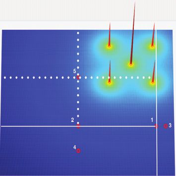
BO algorithm takes as inputs a kernel function, and an ex-                  Widening techniques for MCTS in continuous action
ploration parameter, and assumes that the objective function             spaces There are progressive-widening (PW) algorithms
is a sample from a Gaussian Process (GP). It builds an ac-               that extend MCTS to continuous action spaces (Couëtoux
quisition function, such as upper-confidence-bound function               et al. 2011; Auger, Couëtoux, and Teytaud 2013), but unlike
in GP - UCB (Srinivas et al. 2010), and it chooses to evalu-             the approaches above, their main concern is deciding when
ate, at every iteration, the point that has the highest acqui-           to sample a new action, instead of which action to sample.
sition function value, updates the parameters of the GP, and             The action-sampler in these PW algorithms is assumed to
repeats. The trouble with these approaches is that at every              be an external function that has a non-zero probability of
iteration, they require finding the global optimum of the ac-             sampling a near-optimal action, such as a uniform-random
quisition function, which is expensive in high dimensions.               sampler.
In contrast, VOO does not require an auxiliary optimization                 Typically, a PW technique (Couëtoux et al. 2011) ensures
step.                                                                    that the ratio between the number of sampled actions in a
   There have been several attempts to extend BO to high-                node to the number of visits to the node is above a given
dimensional search spaces (Wang et al. 2013; Kandasamy,                  threshold. In (Auger, Couëtoux, and Teytaud 2013), the au-
Schneider, and Poczos 2015). However, they make a rather                 thors show that a form of PW can guarantee that each state’s
strong assumption on the objective function, such as that                estimated value approaches the optimal value asymptoti-
it lies on a low-dimensional manifold, or that it can be                 cally. However, this analysis does not take into consideration
represented by a linear combination of functions of sub-                 the regret of the action sampler, and assumes that the proba-
dimensions, which are unlikely to hold in domains such as                bility of sampling a near-optimal action is the same in every
robotics, where all of the action dimensions contribute to               visit to the node. So, if an efficient action-sampler, whose re-
its value. Also, these methods require extra hyperparam-                 gret reduces quickly at each visit, is used, their error bound
eters that define the lower-dimensional search space that                 would be very loose. Our analysis shows how the regret of
are tricky to tune. VOO requires neither the assumption or               VOO affects the planning performance.
the hyperparameters for defining the low-dimensional search
space.                                                                          Monte Carlo planning in continuous
   There are also methods that try to combine BO and hi-                               state-action spaces
erarchical partitioning methods, such as (Wang et al. 2014;
Kawaguchi, Kaelbling, and Lozano-Pérez 2015). The idea is               We have a continuous state space S, a continuous action
to use hierarchical partitioning methods to optimize the ac-             space U , a deterministic transition model of the environ-
quisition function of BO; unfortunately, for the same reason             ment, T : S × U → S, a deterministic reward function
as hierarchical partitioning methods, they tend to perform               R : S × U → R, and a discount factor γ ∈ [0, 1). Our
poorly in higher dimensional spaces.                                     objective is to find a sequence of actions with planning hori-
   Optimal planning in continuous spaces using BBFO                      zon H that maximizes
                                                                                          H−1 the sum of the discounted rewards
There are two approaches to continuous-space planning                    maxu0 ,··· ,uH−1 t=0 γ t r(st , ut ) where st+1 = T (st , ut ).
problems that use black-box function-optimization (BBFO)                 Our approach to this problem is to use MCTS with an action-
algorithms. In the first group of approaches, the entire se-              optimization agent, which is an instance of a black-box
quence of actions is treated as a single search space for opti-          function-optimization algorithm, at each node in the tree.
mization. In (Weinstein and Littman 2012), the authors pro-                 We now describe the general MCTS algorithm for con-
pose hierarchical open-loop optimistic planning (HOLOP),                 tinuous state-action spaces, which is given in Algorithm 1.
which uses HOO for finding finite-horizon plans in stochas-                The algorithm takes as inputs an initial state s0 , an action-
tic environments with continuous action space. In (Buşoniu              optimization algorithm A, the total number of iterations
et al. 2011), the authors propose an algorithm called simul-             Niter , the re-evaluation parameter Nr ∈ [0, Niter ], and its
taneous optimistic optimization for planning (SOOP), that                decaying factor κr ∈ [0, 1]. It begins by initializing the nec-
uses SOO to find a plan when the environment is determinis-               essary data in the root node. U denotes the set of actions that
tic. These methods become very expensive as the length of                have been tried at the initial node, Q̂ denotes the estimated
the action sequence increases.                                           state-action value of the sampled actions, and nr denotes the
   The second group of approaches, where our method be-                  number of times we re-evaluated the last-sampled action. It
longs, performs a sample-based tree search with a form of                then performs Niter Monte Carlo simulations, after which it
continuous-space optimizer at each node. Our work most                   returns the apparently best action, the one with the highest
closely resembles hierarchical optimistic optimization ap-               estimated state-action value. This action is executed, and we
plied to trees (HOOT) (Mansley, Weinstein, and Littman                   re-plan in the resulting state.
2011), which applies hierarchical optimistic optimization                   Procedure SIMULATE is shown in Algorithm 2. It is a re-
(HOO) at every node in MCTS for the action-optimization                  cursive function whose termination condition is either en-
problem, but does not provide any performance guaran-                    countering an infeasible state or reaching a depth limit. At
tees. These algorithms have been limited to problems with                the current node T (s), it either selects the action that was
low-dimensional action space, such as the inverted pendu-                most recently sampled, if it has not yet been evaluated Nr
lum. Our experiments demonstrate VOOT can solve prob-                    times and we are not in the last layer of the tree, or it samples
lems with higher-dimensional action spaces much more ef-                 a new action. To sample a new action, it calls A with esti-
ficiently than these algorithms.                                          mated Q-values of the previously sampled actions, T (s).Q̂.

                                                                  9918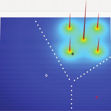
Algorithm 1 MCTS(s0 , A, Niter , Nr , κr , H, γ)                        sampled actions to explore further. In this case, the objective
 1:   global variables: T, R, H, γ, A, Niter , κr , H, γ                for allocating trials is to find the highest-value action among
                                                                        a discrete set, not to obtain accurate estimates of the values
 2:   T (s0 ) = {U = ∅, Q̂(s0 , ·) = −∞, nr = 0}
                                                                        of all the actions.
 3:   for i = 1 → Niter
                                                                           VOOT operates in continuous action spaces but performs
 4:      SIMULATE(s0 , 0, Nr )
                                                                        much more sophisticated value-driven sampling of the con-
 5:   return argmaxu∈T (s0 ).U T (s0 ).Q̂(s0 , u)                       tinuous actions than PW methods. To do this, it needs ac-
                                                                        curate estimates of the values of the actions it has already
                                                                        sampled, and so we have to allocate trials even to actions
Algorithm 2 SIMULATE(s, h, Nr )                                         that may currently “seem” suboptimal. Our empirical results
 1:   global variables: T, R, H, γ, A, Niter , κr , H, γ                show that this trade-off is worth making, especially in high-
 2:   if s == infeasible or h == H                                      dimensional action spaces.
 3:      return 0
 4:   if (|T (s).U | > 0) ∧ (T (s).nr < Nr ) ∧ (h = H − 1)                       Voronoi optimistic optimization
 5:      // re-evaluate the last added action                           Given a bounded search space X , a deterministic objective
 6:      u = T .U.get last added element()                              function f : X → R and a numerical function evaluation
 7:      T (s).nr = T (s).nr + 1                                        budget n, our goal is to devise an exploration strategy over X
 8:   else                                                              that, after n evaluations, minimizes the simple regret defined
 9:      // Perform action optimization                                 as f (x ) − maxt∈[n] f (xt ), where f (x ) = maxx∈X f (x),
10:      u ∼ A(T (s).Q̂)                                                xt is a point evaluated at iteration t, and [n] is shorthand
11:      T (s).U = T (s).U ∪ {u}                                        for {1, · · · n}. Since our algorithm is probabilistic, we will
12:      T (s).nr = 1                                                   analyze its expected behavior. We define the simple regret of
13:   s = T (s, u)                                                     a probabilistic optimization algorithm A as
14:   r = R(s, u)
15:   Q̂new = r + γ · SIMULATE(s , h + 1, Nr · κr )                                  Rn = f (x ) − Ex1:t ∼A max f (xt )
                                                                                                              t∈[n]
16:   if Q̂new > T (s).Q̂(s, u)
17:      T (s).Q̂(s, u) = Q̂new                                            Our algorithm, VOO (Algorithm 3), operates by implicitly
18:   return T (s).Q̂(s, u)                                             constructing a Voronoi partition of the search space X at
                                                                        each iteration: with probability ω, it samples from the entire
                                                                        search space, to sample from a Voronoi cell with probability
                                                                        proportional to its volume; with probability 1−ω, it samples
A transition is simulated based on the selected action, and             from the best Voronoi cell, which is the one induced by the
the process repeats until a leaf is reached; Q-value updates            current best point, x∗t = arg maxi∈[t] f (xi ).
are performed on a backward pass up the tree if a new solu-
tion with higher value has been found (note that, because the
                                                                        Algorithm 3 VOO(X , ω, d(·, ·), n)
transition model is deterministic, the update only requires
maximization.)                                                           1: for t = 0 → n − 1
   The purpose of the re-evaluations is to mitigate the prob-            2:   Sample ν ∼ U nif [0, 1]
lem of non-stationarity: an optimization algorithm A as-                 3:   if ν ≤ ω or t == 0
sumes it is given evaluations of a stationary underlying func-           4:      xt+1 =U NIF S AMPLE(X )
tion, but it is actually given Q̂(s, at ), whose value changes           5:   else
as more actions are explored in the child sub-tree. This                 6:      xt+1 =S AMPLE B EST VC ELL(d(·, ·))
problem is also noted in (Mansley, Weinstein, and Littman                7:   Evaluate ft+1 = f (xt+1 )
                                                                         8: return arg maxt∈{0,...,n−1} ft
2011). So, we make sure that Q̂(s, at ) ≈ Q∗ (s, at ) before
adding an action at+1 in state s by sampling more actions
at the sub-tree associated with at . Since at the leaf node                It takes as inputs the bounded search space X , the explo-
Q∗ (s, at ) = R(s, at ), we do not need to re-evaluate actions          ration probability ω, a semi-metric d(·, ·), and the budget
in leaf nodes. In section 5, we analyze the impact of the es-           n. The algorithm has two sub-procedures. The first one is
timation error in Q̂ on the performance at the root node.               U NIF S AMPLE, which samples a point from X uniformly at
   One may wonder if it is worth it to evaluate the sam-                random, and S AMPLE B EST VC ELL, which samples from the
pled actions same number of times, instead of more sophis-              best Voronoi cell uniformly at random. The former imple-
ticated methods such as Upper Confidence Bound (UCB),                    ments exploration using the Voronoi bias, and the latter im-
for the purpose of using an action-optimization algorithm               plements exploitation of the current knowledge of the func-
A. Typical continuous-action tree search methods perform                tion. Procedure S AMPLE B EST VC ELL can be implemented
progressive widening (PW) (Couëtoux et al. 2011; Auger,                using a form of rejection sampling, where we sample a point
Couëtoux, and Teytaud 2013), in which they sample new                  x at random from X and reject samples until d(x, x∗t ) is the
actions from the action space uniformly at random, but use              minimum among all the distances to the evaluated points.
UCB-like strategies for selecting which of the previously-              Efficiency can be increased by sampling from a Gaussian

                                                                 9919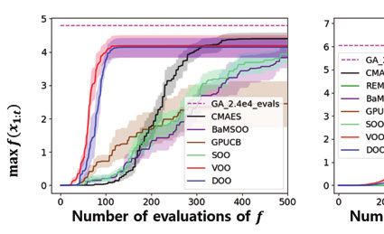
centered at x∗t , which we found to be effective in our exper-              cells decrease in diameter as more points are evaluated in-
iments.                                                                     side of them and that each shell is well-shaped, in that it al-
   To use VOO as an action optimizer in Algorithm 2, we                     ways contains a ball. Our assumption is similar, except that
simply let U be the search space, and use the semi-metric                   in our case, A3 and A4 are stated in terms of expectation,
d(·, ·). f (·) is now the value function Q∗ (s, ·) at each node             because VOO is a probabilistic algorithm.
of the tree, whose estimation is Q̂(s, ·). The consequence                     A5 is an additional assumption that previous literature
of having access only to Q̂ instead of the true optimal state-              has not made. It assumes the existence of a ball inside of
action value function Q∗ will be analyzed in the next section.              which, as you get closer to an optimum, the function values
                                                                            increase. It is possible to drastically relax this assumption to
              Analysis of VOO and VOOT                                      the existence of a sequence of open sets, instead of a ball,
                                                                            whose values increase as you get closer to an optimum. In
We begin with definitions. We denote the set of all global                   our proof, we prove the regret of VOO in this general case,
optima as X  , the Voronoi cell generated by a point x as                  and Theorem 1 holds as the special case when A5 is as-
C(x). We define the diameter of C(x) as supy∈C(x) d(x, y)                    sumed. We present this particular version for the purpose of
where d(·, ·) is the semi-metric on X .                                     brevity and comprehensibility, at the expense of generality.
   Suppose that we have a Voronoi cell generated by                            Define νmin = min∈[k] ν . We have the following regret
x, C0 (x). When we randomly sample a point z from                           bound for VOO. All the proofs are in the appendix.
C0 (x), this will create two new cells, one generated by
x, which we denote with C1 (x), and the other generated                     Theorem 1. Let n be the total number of evaluations. If
                                                                                       1−λ1/k
by z, denoted C1 (z). The diameters of these new cells                      μ̄B (νmin )+1−μ̄B (η·λδmax ) < ω, we have
would be random variables, because z was sampled ran-                                                                       n
domly. Now suppose that we have sampled a sequence                             Rn ≤Lδmax C1 λ1/k + ω(1 − μ̄B (η · λn δmax ))
of n0 points from the sequence of Voronoi cells gener-
ated by x, {C0 (x), C1 (x), C2 (x), · · · , Cn0 (x)}. Then, we de-                    + Lδmax C2 [(1 − ωk μ̄B (νmin )) · (1 + λ1/k )]n
fine the expected diameter of a Voronoi cell generated by
x as the expected value of the diameter of the last cell,                   where C1 and C2 are constants as follows
E[supy∈Cn0 (x) d(x, y)].                                                                                   1
   We write δmax for the largest distance between two points                  C1 :=                                                   ,
                                                                                    1−    ρ(λ1/k+ 1 − [1 − ω + ω μ̄B (η · λδmax )])−1
in X , Br (x) to denote a ball with radius r centered at point
                                                                               ρ := 1 − ω μ̄B (νmin ),
x, and μ̄B (r) = μ(B   r (·))
                    μ(X ) where μ(·) is a Borel measure de-
fined on X . We make the following assumptions:                                                       λ−1/k + 1
                                                                            and C2 :=
A 1. (Translation-invariant semi-metric) d : X × X → R+                                  (λ−1/k + 1) − (1 − ω μ̄B (νmin ))−1
is such that ∀x, y, z ∈ X , d(x, y) = d(y, x), d(x, y) = 0 if
and only if x = y, and d(x + z, y + z) = d(x, y).                              Some remarks are in order. Define an optimal cell as the
A 2. (Local smoothness of f ) There exists at least one global              the cell that contains a global optimum. Intuitively speak-
optimum x ∈ X of f such that ∀x ∈ X , f (x ) − f (x) ≤                    ing, when our best cell is an optimal cell, the regret should
L · d(x, x ) for some L > 0.                                               reduce quickly because when we sample from the best cell
                                                                            with probability 1 − ω, we always sample from the optimal
A 3. (Shrinkage ratio of the Voronoi cells) Consider any                    cell, and we can reduce our expected distance to an optimum
point y inside the Voronoi cell C generated by the point x0 ,               by λ. And because of A5, the best cell is an optimal cell if
and denote d0 = d(y, x0 ). If we randomly sample a point x1                 we have a sample inside one of Bν (x ).
from C, we have E[min(d0 , d(y, x1 ))] ≤ λd0 for λ ∈ (0, 1).
                                                                               Our regret bound verifies this intuition: the first term de-
A 4. (Well-shaped Voronoi cells) There exists η > 0 such                    creases quickly if λ is close to 0, meaning that if we sample
that for any Voronoi cell generated by x with expected di-                  from an optimal cell, then we can get close to the optimum
ameter d0 contains a ball of radius ηd0 centered at x.                      very quickly. The second term says that, if μ̄B (νmin ), the
A 5. (Local symmetry near optimum) X consists of finite                     minimum probability that the best cell is an optimal cell, is
                                                          ()               large, then the regret reduces quickly. We now have the fol-
number of disjoint and connected components {X }k=1 ,
k < ∞. For each component, there exists an open ball                        lowing corollary showing that VOO is no-regret under certain
       ()                ()      ()                     ()              conditions on λ and μ̄B (νmin ).
Bν (x ) for some x ∈ X such that d(x, x ) ≤
                                                                                                     λ1/k
       ()
d(y, x ) implies f (x) ≥ f (y) for any x, y ∈ Bν (x ).
                                                           ()              Corollary 1. If   (1+λ1/k )kμ̄B (νmin )
                                                                                                                      < ω < 1 − λ1/k and
                                                                             λ1/k
   We now describe the relationship between these assump-                   1−λ2/k
                                                                                     < k μ̄B (νmin ), then limn→∞ Rn = 0.
tions and those used in the previous literature. A1 and A2
are assumptions also made in (Munos 2011). These make                          The regret bound of VOOT makes use of the regret bound
the weaker version of the Lipschitz assumption applied only                 of VOO. We have the following theorem.
to the global optima, instead of every pair of points in X .                Theorem 2. Define Cmax = max{C1 , C2 }. Given a de-
A3 and A4 are also very similar to the assumptions made                     creasing sequence η(h) with respect to h, η(h) > 0, h ∈
in (Munos 2011). In (Munos 2011), the author assumes that                   {0 · · · H − 1} and the range of ω as in Theorem 1, if

                                                                     9920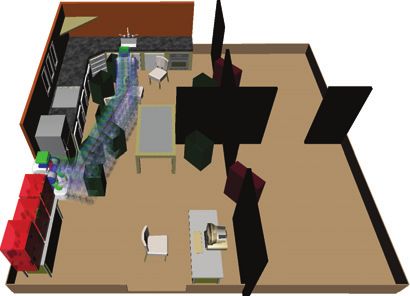
H−1
Niter =      h=0    Nr (h) is used, where
                    η(h) − γη(h + 1)
 Nr (h) ≥ log                               · min(Gλ,ω , Kν,ω,λ )
                         2Lδmax Cmax
Gλ,ω = (log λ1/k + ω )−1 , and Kν,ω,λ = (log([(1 −
ω μ̄B (νmin ))(1 + λ1/k )]))−1 , then for any state s traversed
in the search tree we have
     (h)           (h)
   V (s) − V̂Nr (h) (s) ≤ η(h)        ∀h ∈ {0, · · · , H − 1}
   This theorem states that if we wish to guarantee a regret
of η(h) at each height of the search tree, then we should use
Niter number of iterations, with Nr (h) number of iterations
at each node of height h.
   To get an intuitive understanding of this, we can view the
action optimization problem at each node as a BBFO prob-
lem that takes account of the regret of the next state. To see
this more concretely, suppose that H = 2. First consider a
leaf node, where the problem reduces to a BBFO problem                      Figure 3: Griewank, Rastrigin, and Shekel functions (top to
because there is no next state, and the regret of the node is               bottom) in 3, 10, and 20 dimensions (left to right)
equivalent to the regret of VOO. We can verify that by sub-
stituting Nr (H − 1) to the bound in Theorem 1 the regret of
η(H − 1) is guaranteed. Now suppose that we are at the root                 GP - UCB is used, then its regret bound can be readily used by
node at height H − 2. There are two factors that contribute                 computing the respective Nr (h) values in Theorem 1, and
to the regret at this node: the regret at the next state in height          its own Nr value in Remark 1. It is possible to prove a simi-
H − 1, and the regret that stems from sampling non-optimal                  lar remark in an undiscounted case. Please see Remark 2 in
actions in this node, which is the regret of VOO. Because all               our appendix.
nodes at height H −1 have a regret of η(H −1), to obtain the
regret of η(H − 2), the regret of VOO at the node at height                                       Experiments
H − 2 must be η(H − 2) − γNr (H − 1). Again, by substi-
                                                                            We designed a set of experiments with two goals: (1) test the
tuting Nr (H − 2) to the bound in Theorem 1, we can verify
                                                                            performance of VOO on high-dimensional functions in com-
that that it would yield the regret of η(H − 2) − γNr (H − 1)
                                                                            parison to other black-box function optimizers and (2) test
as desired.
                                                                            the performance of VOOT on deterministic planning prob-
   Now, we have the following remark that relates the de-
                                                                            lems with high-dimensional action spaces in comparison to
sired constant regret at each node and the total number of
                                                                            other continuous-space MCTS algorithms. All plots show
iterations.
                                                                            mean and 95% confidence intervals (CIs) resulting from
Remark 1. If we set η(h) = η, ∀h ∈ {0 · · · H − 1}, and                     multiple executions with different random seeds.
Niter = (Nr )H where
                   η(1 − γ)
       Nr = log                      · min(Gλ,ω , Kν,ω,λ )                  Budgeted-black-box function optimization We evaluate
                    2Lδmax Cmax                                             VOO on three commonly studied objective functions from
then, for any state s traversed in the search tree we have                  the DEAP (Fortin et al. 2012) library: Griewank, Rastri-
                                                                            gin, and Shekel. They are highly non-linear, with many
       (h)           (h)
     V (s) − V̂Nr (h) (s) ≤ η      ∀h ∈ {0, · · · , H − 1}                 local optima, and can extend to high-dimensional spaces.
                                                                            The true optimum of the Shekel function is not known; to
                                                                            gauge the optimality of our solutions, we attempted to find
   We draw a connection to the case of discrete action space                the optimum for our instances by using a genetic algorithm
with b number of actions. In this case, we can guarantee                    (GA) (Qin and Suganthan 2005) with a very large budget of
zero-regret at the root node if we explore all bH number                    function evaluations.
of possible paths from the root node to leaf nodes. In the                     We compare VOO to GP - UCB, DOO, SOO, CMA - ES, an
continuous case, with assumptions A1-A5, it would require                   evolutionary algorithm (Beyer and Schwefel 2002), REMBO,
sampling infinite number of actions at a leaf node to guaran-                the BO algorithm for high-dimensional space that works
tee zero-regret, rendering achieving zero-regret in problems                by projecting the function into a lower-dimensional mani-
with H > 0 impossible. So, this remark considers a posi-                    fold (Wang et al. 2013), and BAMSOO, which combines BO
tive expected regret of η. It show that to guarantee this, we               and hierarchical partitioning (Wang et al. 2014). All algo-
need to explore at least (Nr )H paths from the root to leaf                 rithms evaluate the same initial point. We ran each of them
nodes, where Nr is determined by the regret-bound of our                    with 20 different random seeds. We omit the comparison to
action-optimization algorithm VOO. Alternatively, if some                   HOO, which reduces to DOO on deterministic functions. We
other action-optimization algorithm such as DOO, SOO, or                    also omit testing REMBO in problems with 3-dimensional

                                                                     9921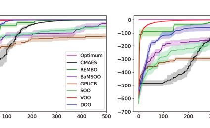
search spaces. Detailed descriptions of the implementations
and extensive parameter choice studies are in the appendix.
   Results are shown in Figure 3. In the 3-dimensional cases,
most algorithms work fairly well with VOO and DOO per-
forming similarly. But, as the number of dimensions in-
creases, VOO is significantly better than all other methods.
Purely hierarchical partitioning methods, DOO and SOO suf-
fers because it is difficult to make the optimal partition,
and SOOsuffers more than DOO because it does not take ad-
vantage of the semi-metric; the mixed approach of BO and
hierarchical partitioning, BAMSOO, tends to do better than
SOO , but still is inefficient in high dimensions for the same
reason as SOO. GP - UCB suffers because in higher dimen-
sions it becomes difficult to globally optimize the acquisi-
tion function. REMBO assumes that the objective function
varies mostly in a lower-dimensional manifold, and there are
negligible changes in the remaining dimensions, but these
assumptions are not satisfied in our test functions, and VOO,             Figure 4: (Top-left) max sum of rewards vs. Niter for the
which doesn’t make this assumption, outperforms it. CMA -                object clearing domain (Bottom-left) that for the packing
ES performs a large number of function evaluations to sus-               domain. (Top-right) minus the number of remaining objects
tain its population, making it less suitable for budgeted-               that need to be moved vs. Niter in the object clearing do-
optimization problems where function evaluations are ex-                 main (Bottom-right) that for the packing domain.
pensive.
   This trend is more pronounced in the Shekel function,
which is flat over most of its domain, but does increase near             lems, PPO (Schulman et al. 2017) and DDPG (Lillicrap et al.
the optimum (see the 2D version in Figure 2). DOO, SOO,                  2016). We train the stochastic policy using the same amount
and BAMSOO perform poorly because they allocate samples                  of simulated experience that the tree-search algorithms use
to large flat regions. GP - UCB performs poorly because in ad-            to find a solution, and report the performance of the best tra-
dition to the difficulty of optimizing the acquisition function,          jectory obtained.
the function is not well modeled by a GP with a typical ker-                 The action-space dimensions are 6 and 9 in the object-
nel, and the same goes for REMBO. VOO has neither of these               clearing and packing domains, respectively. The detailed
problems; as soon as VOO gets a sample that has a slightly               action-space and reward function definitions, and extensive
better value, it can concentrate its sampling to that region,            hyper-parameter value studies are given in the appendix.
which drives it more quickly to the optimum. We do note                  The plots in this section are obtained with 20 and 50 ran-
that CMA - ES is the only method besides VOO to perform at               dom seeds for object-clearing and packing problems, respec-
all well in high-dimensions.                                             tively.
                                                                             We first consider the object-clearing problem (s0 is shown
                                                                         in Figure 1 (right)). Roughly, the reward function penalizes
  Sequential mobile manipulation planning problems                       infeasible actions and actions that move an obstacle but do
We now study two realistic robotic planning problems. We                 not clear it from the path; it rewards actions that clear an
compare VOOT to DOOT, which respectively use VOO and                     object, but with value inversely proportional to the length of
DOO and as its action-optimizer in Algorithm 2, and a                    the clearing motion. The challenging aspect of this problem
single-progressive-widening algorithm that uses UCT (PW-                 is that, to the right of the kitchen area, there are two large
UCT ) (Couëtoux et al. 2011). But to make DOOT work in                  rooms that are unreachable by the robot; object placements
these problems, we consider a randomized variant called                  in those rooms will be infeasible. So, the robot must clear
RAND - DOOT which samples an action uniformly in the cell                obstacles within the relatively tight space of the kitchen.
to be evaluated next, instead of always selecting the mid-                   Figure 4 (Top-left) shows the results. In this case, PW- UCT
point, which could not solve any of these problems.                      samples from the whole space, concentrating far too many
   The objective of comparing to PW- UCT is to verify our                of them in the unreachable empty rooms. RAND - DOOT also
claim that using an efficient action-optimizer, at the expense            spends time partitioning the big unreachable regions, due to
of uniform re-evaluations of the sampled actions, is better              its large exploration bonus; however it performs better than
evaluating sampled actions with UCB at the expense of sam-               PW- UCT because once the cells it makes in the unreachable
pling new actions uniformly. The objective of comparing to               region get small enough, it starts concentrating in the kitchen
RAND - DOOT is to verify our claim that VOOT can scale to                region. However, it performs worse than VOOT for similar
higher dimensional problems for which RAND - DOOT does                   reasons as in the Shekel problems: as soon as VOOT finds the
not.                                                                     first placement inside the kitchen (i.e. first positive reward),
   In addition to the state-of-the-art continuous MCTS meth-             it immediately focuses its sampling effort near this area with
ods, we compare VOO to the representative policy search                  probability 1−ω. This phenomenon is illustrated in Figure 5,
methods typically used for continuous-action space prob-                 which shows the values of placements. We can also observe

                                                                  9922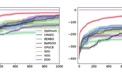
from Figure 4 (Top-right) that VOOT clears obstacles much
faster than the other methods; it clears almost all of them
with 750 simulations, while others require more than 1700,
which is about a factor of 2.3 speed-up.
   The reinforcement learning algorithms, PPO and DDPG,
perform poorly compared to the tree-search methods. We
can see that within the first 250 simulations, their rewards
grow just as quickly as for the search algorithms, but they
seem to get stuck at local optima, clearing only one or two                     Figure 5: Q̂(s, a) of PW- UCT, RAND - DOOT, and VOOT (left
obstacles. This is because the problem has two challenging                      to right) after 50 visits to the place node for the first ob-
characteristics: large future delayed rewards and sparse re-                    ject. Blue and purple bars indicate values of infeasible and
wards.                                                                          feasible placements, respectively. Solid robot indicates the
   The problem has sparse rewards because most of the ac-                       current state of the robot, and the transparent robots indicate
tions are unreachable placements, or kinematically infeasi-                     the placements sampled. Notice VOOT has far fewer samples
ble picks. It has large delayed rewards because the reward                      in infeasible regions.
function is inversely proportional to the length of the clear-
ing motion, but the first few objects need to be moved far
away from their initial locations to make the subsequent ob-                    rive a performance guarantee on VOOT. The tree perfor-
jects accessible. Unfortunately, the RL methods come with                       mance guarantee is the first of its kind for search methods
an ineffective exploration strategy for long-horizon planning                   with BBFO-type algorithms at the nodes. We demonstrated
problems: Gaussian random actions1 . This strategy could                        that both VOO and VOOT significantly outperform previous
not discover the delayed future rewards, and the policies fell                  methods within a small number of iterations in challenging
into a local optima in which they try to clear the first two                     higher-dimensional synthetic BBFO and practical robotics
objects with the least possible cost, but blocking the way to                   problems.
the subsequent objects.                                                            We believe there is a strong potential for combining learn-
   We now consider the conveyor belt problem (s0 shown                          ing and VOOT to tackle more challenging tasks in continu-
in Figure 1 (left)). The challenge is the significant interde-                   ous domains, much like combining learning and Polynomial
pendence among the actions at different time steps: the first                    UCT has done in the game of Go (Silver et al. 2016). We
two boxes are too big to go through the door that leads to                      can learn from previous planning experience a policy πθ ,
the bigger rooms, so the robot must place them in the small                     which assigns high probabilities to promising actions, using
first room, so that there is still room to move the rest of the                  a reinforcement-learning algorithm. We can then use VOO
objects into the bigger rooms. Figure 4 (Bottom-left) shows                     with πθ , instead of uniform sampling.
the results. VOOT achieves the reward of a little more than
3 with 1000 simulations, while other methods achieve be-                                           Acknowledgement
low 1 ; even with 3000 simulations, their rewards are below
2, whereas that of VOOT goes up to approximately 4. Fig-                        We gratefully acknowledge support from NSF grants
ure 4 (Bottom-right) shows that VOOT finds a way to place                        1523767 and 1723381; from AFOSR grant FA9550-17-1-
as many as 15 objects within 1000 simulations, whereas the                      0165; from ONR grant N00014-18-1-2847; from Honda Re-
alternative methods have only found plans for placing 12                        search; and from the MIT-Sensetime Alliance on AI. Any
or 13 objects after 3000 simulations. We view each action-                      opinions, findings, and conclusions or recommendations ex-
optimization problem (line 10 of Alg. 2) as a BBFO prob-                        pressed in this material are those of the authors and do not
lem, since we only have access to the values of the actions                     necessarily reflect the views of our sponsors.
that have been simulated, and the number of simulations is
limited to Niter . The RL approaches suffer in this problem                                             References
as well, packing at most 8 boxes, while the worst search-                       Auger, D.; Couëtoux, A.; and Teytaud, O. 2013. Continuous
based method packs 13 boxes. Again, the reason is the same                      Upper Confidence Trees with polynomial exploration - con-
as in the previous domain: sparse and delayed long-term re-                     sistency. Joint European Conference on Machine Learning
wards.                                                                          and Knowledge Discovery in Databases.
                                                                                Beyer, H.-G., and Schwefel, H.-P. 2002. Evolution strategies
             Future work and conclusions                                        – a comprehensive introduction. Natural Computing.
We proposed a continuous MCTS algorithm in determinis-                          Bubeck, S.; Munos, R.; Stoltz, G.; and Szepesvári, C. 2011.
tic environments that scales to higher-dimensional spaces,                      X-armed bandits. Journal of Machine Learning Research.
which is based on a novel and efficient BBFO VOO. We                             Buşoniu; Daniels, A.; Munos, R.; and Babus̆ka, R. 2011.
proved a bound on the regret for VOO, and used it to de-                        Optimistic planning for continuous-action deterministic sys-
    1                                                                           tems. IEEE Symposium on Adaptive Dynamic Programming
      In order to get the RL methods to perform at all well, we had to
tailor the exploration strategy to compensate for the fact that many
                                                                                and Reinforcement Learning.
of the action choices are completely infeasible. Details are in the             Couëtoux, A.; Hoock, J.-B.; Sokolovska, N.; Teytaud, O.;
appendix.                                                                       and Bonnard, N. 2011. Continuous upper confidence trees.

                                                                         9923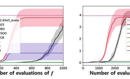
International Conference on Learning and Intelligent Opti-                Weinstein, A., and Littman, M. 2012. Bandit-based planning
mization.                                                                 and learning in continuous-action markov decision proce-
Fortin, F.-A.; De Rainville, F.-M.; Gardner, M.-A.; Parizeau,             ses. International Conference on Automated Planning and
M.; and Gagné, C. 2012. DEAP: Evolutionary algorithms                    Scheduling.
made easy. Journal of Machine Learning Research.
Kandasamy, K.; Schneider, J.; and Poczos, B. 2015. High
dimensional bayesian optimisation and bandits via additive
models. International Conference on Machine Learning.
Kawaguchi, K.; Kaelbling, L.; and Lozano-Pérez, T. 2015.
Bayesian optimization with exponential convergence. In Ad-
vances in Neural Information Processing Systems.
Kuffner, J., and LaValle, S. 2000. RRT-connect: An effi-
cient approach to single-query path planning. In Interna-
tional Conference on Robotics and Automation.
Lillicrap, T. P.; J. J. Hunt, A. P.; Heess, N.; Erez, T.; Tassa,
Y.; Silver, D.; and Wierstra, D. 2016. Continuous control
with deep reinforcement learning. International Conference
on Learning Representations.
Mansley; Weinstein, A.; and Littman, M. 2011. Sample-
based planning for continuous action Markov Decision Pro-
cesses. International Conference on Automated Planning
and Scheduling.
Munos, R. 2011. Optimistic optimization of a deterministic
function without the knowledge of its smoothness. Advances
in Neural Information Processing Systems.
Munos, R. 2014. From bandits to Monte-Carlo Tree Search:
the optimistic principle applied to optimization and plan-
ning. Foundations and Trends in Machine Learning.
Pintér, J. 1996. Global Optimization in Action (Contin-
uous and Lipschitz Optimization: Algorithms, Implementa-
tions and Applications). Springer US.
Qin, A., and Suganthan, P. 2005. Self-adaptive differen-
tial evolution algorithm for numerical optimization. IEEE
Congress on Evolutionary Computation.
Schulman, J.; Wolski, F.; Dhariwal, P.; Radford, A.; and
Klimov, O. 2017. Proximal policy optimization algorithms.
arXiv.
Silver, D.; Huang, A.; Maddison, C.; Guez, A.; Sifre, L.;
van den Driessche, G.; Schrittwieser, J.; Antonoglou, I.;
Panneershelvam, V.; Lanctot, M.; Dieleman, S.; Grewe, D.;
Nham, J.; Kalchbrenner, N.; Sutskever, I.; Lillicrap, T.;
Leach, M.; Kavukcuoglu, K.; Graepel, T.; and Hassabis, D.
2016. Mastering the game of Go with deep neural networks
and tree search. Nature.
Srinivas, N.; Krause, A.; Kakade, S.; and Seeger, M. 2010.
Gaussian Process optimization in the bandit setting: no re-
gret and experimental design. International Conference on
Machine Learning.
Wang, Z.; Zoghi, M.; Hutter, F.; Matheson, D.; and Freitas,
N. 2013. Bayesian optimization in high dimensions via
random embeddings ziyu. International Conference on Ar-
tificial Intelligence and Statistics.
Wang, Z.; Shakibi, B.; Jin, L.; and Freitas, N. 2014.
Bayesian multi-scale optimistic optimization. International
Conference on Artificial Intelligence and Statistics.

                                                                   9924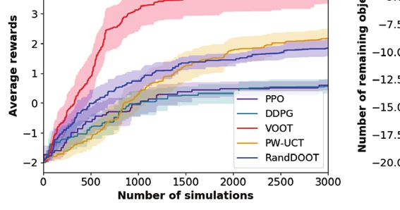
You can also read