Mixed Variable Bayesian Optimization with Frequency Modulated Kernels
←
→
Page content transcription
If your browser does not render page correctly, please read the page content below
Mixed Variable Bayesian Optimization with Frequency Modulated Kernels

                Changyong Oh1                         Efstratios Gavves1                        Max Welling1,2

                     1 Informatics   Institute, University of Amsterdam, Amsterdam, The Netherlands
                           2 Qualcomm     AI Research Netherlands, Amsterdam, The Netherlands

                        Abstract                                  ter optimization tasks of machine learning algorithms (e.g.
                                                                  Alpha-Go [Chen et al., 2018]). Much of this success is
                                                                  attributed to the flexibility and the quality of uncertainty
    The sample efficiency of Bayesian optimiza-                   quantification of Gaussian Process (GP)-based surrogate
    tion (BO) is often boosted by Gaussian Pro-                   models [Snoek et al., 2012, Swersky et al., 2013, Oh et al.,
    cess (GP) surrogate models. However, on mixed                 2018].
    variable spaces, surrogate models other than GPs
    are prevalent, mainly due to the lack of kernels              Despite the superiority of GP surrogate models, as compared
    which can model complex dependencies across dif-              to non-GP ones, their use on spaces with discrete struc-
    ferent types of variables. In this paper, we propose          tures (e.g., chemical spaces [Reymond and Awale, 2012],
    the frequency modulated (FM) kernel flexibly mod-             graphs and even mixtures of different types of spaces) is
    eling dependencies among different types of vari-             still application-specific [Kandasamy et al., 2018, Korovina
    ables, so that BO can enjoy the further improved              et al., 2019]. The main reason is the difficulty of defining ker-
    sample efficiency. The FM kernel uses distances on            nels flexible enough to model dependencies across different
    continuous variables to modulate the graph Fourier            types of variables. On mixed variable spaces which consist
    spectrum derived from discrete variables. How-                of different types of variables including continuous, ordinal
    ever, the frequency modulation does not always                and nominal variables, current BO approaches resort to non-
    define a kernel with the similarity measure behav-            GP surrogate models, such as simple linear models or linear
    ior which returns higher values for pairs of more             models with manually chosen basis functions [Daxberger
    similar points. Therefore, we specify and prove               et al., 2019]. However, such linear approaches are limited
    conditions for FM kernels to be positive definite             because they may lack the necessary model capacity.
    and to exhibit the similarity measure behavior. In            There is much progress on BO using GP surrogate mod-
    experiments, we demonstrate the improved sample               els (GP BO) for continuous, as well as for discrete variables.
    efficiency of GP BO using FM kernels (BO-FM).                 However, for mixed variables it is not straightforward how
    On synthetic problems and hyperparameter opti-                to define kernels ,which can model dependencies across
    mization problems, BO-FM outperforms competi-                 different types of variables. To bridge the gap, we propose
    tors consistently. Also, the importance of the fre-           frequency modulation which uses distances on continuous
    quency modulation principle is empirically demon-             variables to modulate the frequencies of the graph spectrum
    strated on the same problems. On joint optimiza-              [Ortega et al., 2018] where the graph represents the discrete
    tion of neural architectures and SGD hyperparam-              part of the search space [Oh et al., 2019].
    eters, BO-FM outperforms competitors including
    Regularized evolution (RE) and BOHB. Remark-                  A potential problem in the frequency modulation is that it
    ably, BO-FM performs better even than RE and                  does not always define a kernel with the similarity measure
    BOHB using three times as many evaluations.                   behavior [Vert et al., 2004]. That is, the frequency mod-
                                                                  ulation does not necessarily define a kernel that returns
                                                                  higher values for pairs of more similar points. Formally, for
1   INTRODUCTION                                                  a stationary kernel k(x, y) = s(x − y), s should be decreas-
                                                                  ing [Remes et al., 2017]. In order to guarantee the similar-
Bayesian optimization has found many applications rang-           ity measure behavior of kernels constructed by frequency
ing from daily routine level tasks of finding a tasty cookie      modulation, we stipulate a condition, the frequency modula-
recipe [Solnik et al., 2017] to sophisticated hyperparame-

                     Accepted for the 37th Conference on Uncertainty in Artificial Intelligence (UAI 2021).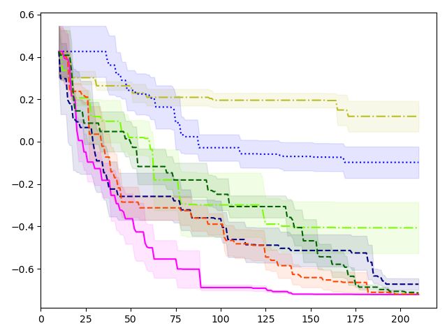
tion principle. Theoretical analysis results in proofs of the        exploitation trade-off [Shahriari et al., 2015]. Compared
positive definiteness as well as the effect of the frequency         with other surrogate models (such as Random Forest [Hutter
modulation principle. We coin frequency modulated (FM)               et al., 2011] and a tree-structured density estimator [Bergstra
kernels as the kernels constructed by frequency modulation           et al., 2011]), Gaussian Processes (GPs) tend to yield better
and respecting the frequency modulation principle.                   results [Snoek et al., 2012, Oh et al., 2018].
Different to methods that construct kernels on mixed vari-           For a given kernel k and data D = (X, y) where X =
ables by kernel addition and kernel multiplication, for exam-        [x1 , · · · , xn ]T and y = [y1 , · · · , yn ]T , a GP has a predic-
ple, FM kernels do not impose an independence assumption             tive mean µ(x∗ |X, y) = k∗X (kXX + σ 2 I)−1 y and predic-
among different types of variables. In FM kernels, quantities        tive variance σ 2 (x∗ |X, y) = k∗∗ − k∗X (kXX + σ 2 I)−1 kX∗
in the two domains, that is the distances in a spatial domain        where k∗∗ = k(x∗ , x∗ ), [k∗X ]1,i = k(x∗ , xi ), kX∗ = (k∗X )T and
and the frequencies in a Fourier domain, interact. Therefore,        [kXX ]i, j = k(xi , x j ).
the restrictive independence assumption is circumvented,
and thus flexible modeling of mixed variable functions is
                                                                     2.2     KERNELS ON DISCRETE VARIABLES
enabled.
In this paper, (i) we propose frequency modulation, a new            We first review some kernel terminology [Scholkopf and
way to construct kernels on mixed variables, (ii) we provide         Smola, 2001] that is needed in the rest of the paper.
the condition to guarantee the similarity measure behavior of        Definition 2.1 (Gram Matrix). Given a function k :
FM kernels together with a theoretical analysis, and (iii) we        X × X → R and data x1 , · · · , xn ∈ X , the n × n matrix
extend frequency modulation so that it can model complex             K with elements [K]i j = k(xi , x j ) is called the Gram matrix
dependencies between arbitrary types of variables. In exper-         of k with respect to x1 , · · · , xn .
iments, we validate the benefit of the increased modeling
                                                                     Definition 2.2 (Positive Definite Matrix). A real n × n ma-
capacity of FM kernels and the importance of the frequency
                                                                     trix K satisfying ∑i, j ai [K]i j a j ≥ 0 for all ai ∈ R is called
modulation principle for improved sample efficiency on dif-
ferent mixed variable BO tasks. We also test BO with GP              positive definite (PD)1 .
using FM kernels (BO-FM) on a challenging joint optimiza-            Definition 2.3 (Positive Definite Kernel). A function k :
tion of the neural architecture and the hyperparameters with         X × X → R which gives rise to a positive definite Gram
two strong baselines, Regularized Evolution (RE) [Real               matrix for all n ∈ N and all x1 , · · · , xn ∈ X is called a posi-
et al., 2019] and BOHB [Falkner et al., 2018]. BO-FM                 tive definite (PD) kernel, or simply a kernel.
outperforms both baselines which have proven their com-
petence in neural architecture search [Dong et al., 2021].           A search space which consists of discrete variables, includ-
Remarkably, BO-FM outperforms RE with three times eval-              ing both nominal and ordinal variables, can be represented
uations.                                                             as a graph [Kondor and Lafferty, 2002, Oh et al., 2019]. In
                                                                     this graph each vertex represents one state of exponentially
                                                                     many joint states of the discrete variables. The edges repre-
2     PRELIMINARIES                                                  sent relations between these states (e.g. if they are similar)
                                                                     [Oh et al., 2019]. With a graph representing a search space
2.1   BAYESIAN OPTIMIZATION WITH
                                                                     of discrete variables, kernels on a graph can be used for
      GAUSSIAN PROCESSES
                                                                     BO. In [Smola and Kondor, 2003], for a positive decreasing
Bayesian optimization (BO) aims at finding the global opti-          function f and a graph G = (V , E ) whose graph Laplacian
mum of a black-box function g over a search space X . At             L(G )2 has the eigendecomposition UΛU T , it is shown that
each round BO performs an evaluation yi on a new point xi ∈          a kernel can be defined as
X , collecting the set of evaluations D t = {(xi , yi )}i=1,··· ,t                    kdisc (v, v0 |β ) = [U f (Λ|β )U T ]v,v0                (1)
at the t-th round. Then, a surrogate model approximates the
function g given D t using the predictive mean µ(x∗ | D t )
                                                                     where β ≥ 0 is a kernel parameter and f is a positive de-
and the predictive variance σ 2 (x∗ | D t ). Now, an acquisi-
                                                                     creasing function. It is the reciprocal of a regularization
tion function r(x∗ ) = r(µ(x∗ | D t ), σ 2 (x∗ | D t )) quantifies
                                                                     operator [Smola and Kondor, 2003] which penalizes high
how informative input x ∈ X is for the purpose of find-
                                                                     frequency components in the spectrum.
ing the global optimum. g is then evaluated at xt+1 =
                                                                           1 Sometimes,
argmaxx∈X r(x), yt+1 = g(xt+1 ). With the updated set of                                     different terms are used, semi-positive definite
evaluations, D t+1 = D t ∪{(xt+1 , yt+1 )}, the process is re-       for ∑i, j ai [K]i j a j ≥ 0 and positive definite for ∑i, j ai [K]i j a j > 0.
peated.                                                              Here, we stick to the definition in [Scholkopf and Smola, 2001].
                                                                         2 In this paper, we use a (unnormalized) graph Laplacian
A crucial component in BO is thus the surrogate model.               L(G ) = D − A while, in [Smola and Kondor, 2003], symmetric
Specifically, the quality of the predictive distribution of the      normalized graph Laplacian, Lsym (G ) = D−1/2 (D − A)D−1/2 . (A :
surrogate model is critical for balancing the exploration-           adj. mat. / D : deg. mat.) Kernels are defined for both.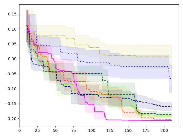
3    MIXED VARIABLE BAYESIAN
     OPTIMIZATION
With the goal of obtaining flexible kernels on mixed vari-
ables which can model complex dependencies across dif-
ferent types of variables, we propose the frequency modu-
lated (FM) kernel. Our objective is to enhance the modelling
capacity of GP surrogate models and, thereby improve the
sample efficiency of mixed-variable BO. FM kernels use
the continuous variables to modulate the frequencies of the
kernel of discrete variables defined on the graph. As a con-                              Figure 1: Influence on eigencomponents
sequence, FM kernels can model complex dependencies
between continuous and discrete variables. Specifically, let                   Definition 3.2 (FM kernel). A FM kernel is a function on
us start with continuous variables of dimension DC , and dis-                  (RDC × V ) × (RDC × V ) of the form in Eq. (2), where f is
crete variables represented by the graph G = (V , E ) whose                    a frequency modulating function on R+ × R.
graph Laplacian L(G ) has eigendecompostion UΛU T . To
define a frequency modulated kernel we consider the func-
tion k : (RDC × V )×(RDC × V ) ⇒ R of the following form                       3.1    FREQUENCY REGULARIZATION OF FM
                                                                                      KERNELS
               k((c, v), (c0 , v0 )|β , θ )
                    |V |                                                       In [Smola and Kondor, 2003], it is shown that Eq. (1) de-
                =   ∑ [U]v,i f (λi , k c − c0 kθ |β )[U]v0 ,i            (2)   fines a kernel that regularizes the eigenfunctions with high
                    i=1                                                        frequencies when f is positive and decreasing. It is also
                            D
where    k c − c0 k2θ C
                 = ∑d=1  (cd − c0d )2 /θd2 and (θ , β ) are tun-               shown that the reciprocal of f in Eq. (1) is a corresponding
able parameters. f is the frequency modulating function                        regularization operator. For example, the diffusion kernel
defined below in Def. 3.1.                                                     defined with f (λ ) = exp(−β λ ) corresponds to the regular-
                                                                               ization operator r(λ ) = exp(β λ ). The regularized Laplacian
The function f in Eq. (2) takes frequency λi and distance                      kernel defined with f (λ ) = 1/(1 + β λ ) corresponds to the
k c − c0 k2θ as arguments, and its output is combined with the                 regularization operator r(λ ) = 1 + β λ . Both regularization
basis [U]v,i . That is, the function f processes the informa-                  operators put more penalty on higher frequencies λ .
tion in each eigencomponent separately while Eq. (2) then
sums up the information processed by f . Note that unlike                      Therefore, the property FM-P1 forces FM kernels to have
kernel addition and kernel product,3 , the distance k c − c0 k2θ               the same regularization effect of promoting a smoother func-
influences each eigencomponent separately as illustrated in                    tion by penalizing the eigenfunctions with high frequencies.
Figure.1. Unfortunately, Eq. (2) with an arbitrary function
 f does not always define a positive definite kernel. More-                    3.2    POSITIVE DEFINITENESS OF FM KERNELS
over, Eq. (2) with an arbitrary function f may return higher
kernel values for less similar points, which is not expected                   Determining whether Eq.2 defines a positive definite ker-
from a proper similarity measure [Vert et al., 2004]. To this                  nel is not trivial. The reason is that the gram matrix
end, we first specify three properties of functions f such                     [k((ci , vi ), (c j , v j ))]i, j is not determined only by the entries vi
that Eq. (2) guaranteed to be a positive definite kernel and a                 and v j , but these entries are additionally affected by different
proper similarity measure at the same time. Then, we moti-                     distance terms k ci − c j kθ . To show that FM kernels are pos-
vate the necessity of each of the properties in the following                  itive definite, it is sufficient to show that f (λi , k c − c0 kθ | β )
subsections.                                                                   is positive definite on (c, c0 ) ∈ RDC × RDC .
Definition 3.1 (Frequency modulating function). A fre-                         Theorem 3.1. If f (λ , k c − c0 kθ | β ) defines a positive defi-
quency modulating function is a function f : R+ × R → R                        nite kernel with respect to c and c0 , then the FM kernel with
satisfying the three properties below.                                         such f is positive definite jointly on c and v. That is, the
FM-P1 For a fixed t ∈ R, f (s,t) is a positive and decreasing                  positive definiteness of f (λ , k c − c0 kθ | β ) on RDC implies
      function with respect to s on [0, ∞).                                    the positive definiteness of the FM kernel on RDC × V .
FM-P2 For a fixed s ∈ R+ , f (s, k c − c0 kθ ) is a positive
      definite kernel on (c, c0 ) ∈ RDC × RDC .                                Proof. See Supp. Sec.1, Thm. 1.1.
FM-P3 For t1 < t2 , ht1 ,t2 (s) = f (s,t1 ) − f (s,t2 ) is positive,
      strictly decreasing and convex w.r.t s ∈ R+ .
                                                                               Note that Theorem 3.1 shows that the property FM-P2 guar-
                                                 0 2
    3 e.g    kadd ((c, v), (c0 , v0 )) = e−k c − c kθ + kdisc (v, v0 )   and   antees that FMs kernels are positive definite jointly on c and
                                       0 2
k prod ((c, v), (c0 , v0 )) = e−k c − c kθ · kdisc (v, v0 )                    v.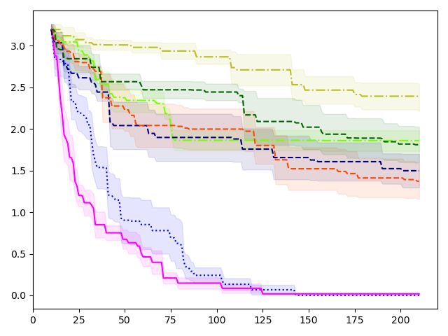
In the current form of Theorem 3.1, the frequency mod-                    h(0)/n + h(n) ∑ni=2 [U]v,i [U]v0 ,i = (h(0) − h(n))/n in which
ulating functions depend on the distance k c − c0 kθ . How-               non-negativity follows with decreasing h.
ever, the proof does not change for the more general form
                                                                          For the complete proof, see Thm. 2.1 in Supp. Sec. 2.
of f (λ , c, c0 |α, β ), where f does not depend on k c − c0 kθ .
Hence, Theorem 3.1 can be extended to the more general
case that f (λ , c, c0 |α, β ) is positive definite on (c, c0 ) ∈         Theorem 3.2 thus shows that the property FM-P3 is suf-
RD C × RD C .                                                             ficient for Eq. (4) to hold. We call the property FM-P3
                                                                          the frequency modulation principle. Theorem 3.2 also im-
                                                                          plies the non-negativity of many kernels derived from graph
3.3   FREQUENCY MODULATION PRINCIPLE                                      Laplacian.

A kernel, as a similarity measure, is expected to return higher           Corollary 3.2.1. The random walk kernel derived from
values for pairs of more similar points and vice versa [Vert              the symmetric normalized Laplacian [Smola and Kondor,
et al., 2004]. We call such behavior the similarity measure               2003], the diffusion kernels [Kondor and Lafferty, 2002, Oh
behavior.                                                                 et al., 2019] and the regularized Laplacian kernel [Smola
                                                                          and Kondor, 2003] derived from symmetric normalized or
In Eq. (2), the distance k c − c0 kθ represents a quantity in
                                                                          unnormalized Laplacian, are all non-negatived valued.
the “spatial” domain interacting with quantities λi s in the
“frequency” domain. Due to the interplay between the two
different domains, the kernels of the form Eq. (2) do not                 Proof. See Cor. 2.1.1 in Supp. Sec. 2.
exhibit the similarity measure behavior for an arbitrary
function f . Next, we derive a sufficient condition on f for              3.4    FM KERNELS IN PRACTICE
the similarity measure behavior to hold for FM kernels.
Formally, the similarity measure behavior is stated as                    Scalability Since the (graph Fourier) frequencies and ba-
                                                                          sis functions are computed by the eigendecomposition of
           k c − c0 kθ ≤ kc̃ − c̃0 kθ                                     cubic computational complexity, a plain application of fre-
             ⇒ k((c, v), (c0 , v0 )) ≥ k((c̃, v), (c̃0 , v0 ))     (3)    quency modulation makes the computation of FM ker-
                                                                          nels prohibitive for a large number of discrete variables.
                                                                          Given P discrete variables where each variable can be in-
or equivalently,                                                          dividually represented by a graph G p , the discrete part of
                                                                          the search space can be represented as a product space,
              k c − c0 kθ ≤ kc̃ − c̃0 kθ                                  V = V 1 × · · · × V P.
                     |V |
                ⇒                                                         In this case, we define FM kernels on RDC × V =
                      ∑ [U]v,i ht1 ,t2 (λi |β )[U]v0 ,i ≥ 0        (4)
                                                                          RDC ×(V 1 × · · · × V P ) as
                     i=1

where ht1 ,t2 (λ |β ) = f (λ ,t1 |β ) − f (λ ,t2 |β ), t1 = k c − c0 kθ                                           P
                                                                            k((c, v), (c0 , v0 )| α, β , θ ) =   ∏ k p ((c, v p ), (c0 , v0p )|β p , θ )
and t2 = kc̃ − c̃0 kθ .
                                                                                                                 p=1

Theorem 3.2. For a connected and weighted undirected                              P |V p |
graph G = (V , E ) with non-negative weights on edges, de-                   =   ∏ ∑ [U p ]v p ,i f (λip , α p k c − c0 kθ |β p )[U p ]v0p ,i         (5)
fine a similarity (or kernel) a(v, v0 ) = [Uh(Λ)U T ]v,v0 , where                p=1 i=1

U and Λ are eigenvectors and eigenvalues of the graph
Laplacian L(G ) = UΛU T . If h is any non-negative and                    where v = (v1 , · · · , vP , v0 = (v01 , · · · , v0P , α = (α1 , · · · , αP )
strictly decreasing convex function on [0, ∞), then a(v, v0 ) ≥           β = (β1 , · · · , βP ) and the graph Laplacian is given as L(G p )
0 for all v, v0 ∈ V .                                                     with the eigendecomposition U p diag[λ1p , · · · , λkpV p k ]U pT .
                                                                          Eq.5 should not be confused with the kernel product of ker-
Therefore, these conditions on h(Λ) result in a similarity                nels on each V p . Note that the distance k c − c0 kθ is shared,
measure a with only positive entries, which in turn proves                which introduces the coupling among discrete variables and
property Eq. (4). Here, we provide a proof of the theorem for             thus allows more modeling freedom than a product kernel.
a simpler case with an unweighted complete graph, where                   In addition to the coupling, the kernel parameter α p s lets us
Eq. (4) holds without the convexity condition on h.                       individually determine the strength of the frequency modu-
                                                                          lation.
Proof. For a unweighted complete graph with n vertices, we
have eigenvalues λ1 √ = 0, λ2 = · · · = λn = n and eigenvectors           Examples Defining a FM kernel amounts to constructing
such that [U]·1 = 1/ n and ∑ni=1 [U]v,i [U]v0 ,i = δvv0 . For v 6=        a frequency modulating function. We introduce examples of
v0 , the conclusion in Eq. (4), ∑ni=1 h(λi )[U]v,i [U]v0 ,i becomes       flexible families of frequency modulating functions.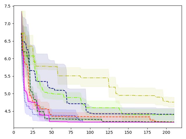
Proposition 1. For S ∈ (0, ∞), a finite measure µ on                                  4   RELATED WORK
[0, S], µ-measurable τ : [0, S] ⇒ [0, 2] and µ-measurable                             On continuous variables, many sophisticated kernels have
ρ : [0, S] ⇒ N, the function of the form below is a frequency                         been proposed [Wilson and Nickisch, 2015, Samo and
modulating function.                                                                  Roberts, 2015, Remes et al., 2017, Oh et al., 2018]. In
           f (λ , αk c − c0 kθ |β )                                                   contrast, kernels on discrete variables have been studied
               Z S                                                                    less [Haussler, 1999, Kondor and Lafferty, 2002, Smola
                                      1                                               and Kondor, 2003]. To our best knowledge, most of exist-
           =                                    τ(s)
                                                                 µ(ds)          (6)
                 0   (1 + β λ + αk c − c0 kθ )ρ(s)                                    ing kernels on mixed variables are constructed by a kernel
                                                                                      product Swersky et al. [2013], Li et al. [2016] with some
                                                                                      exceptions [Krause and Ong, 2011, Swersky et al., 2013,
                                                                                      Fiducioso et al., 2019], which rely on kernel addition.
Proof. See Supp. Sec.3, Prop.1.
                                                                                      In mixed variable BO, non-GP surrogate models are more
                                                                                      prevalent, including SMAC [Hutter et al., 2011] using ran-
Assuming S = 1 and τ(s) = 2, Prop. 1 gives (1 +                                       dom forest and TPE [Bergstra et al., 2011] using a tree
β λ + αk c − c0 k2θ )−1 with ρ(s) = 1 and µ(ds) = ds, and                             structured density estimator. Recently, by extending the
∑Nn=1 an (1 + β λ + αk c − c0 k2θ )−n with ρ(s) = bNsc and                            approach of using Bayesian linear regression for discrete
µ({n/N}) = an ≥ 0 and µ([{n/N}cn=1,··· ,N ) = 0.                                      variables [Baptista and Poloczek, 2018], Daxberger et al.
                                                                                      [2019] proposes Bayesian linear regression with manually
                                                                                      chosen basis functions on mixed variables, providing a re-
3.5    EXTENSION OF THE FREQUENCY                                                     gret analysis using Thompson sampling as an acquisition
       MODULATION                                                                     function. Another family of approaches utilizes a bandit
                                                                                      framework to handle the acquisition function optimization
Frequency modulation is not restricted to distances on Eu-                            on mixed variables with theoretical analysis [Gopakumar
clidean spaces but it is applicable to any arbitrary space with                       et al., 2018, Nguyen et al., 2019, Ru et al., 2020]. Nguyen
a kernel defined on it. As a concrete example of frequency                            et al. [2019] use GP in combination with multi-armed bandit
modulation by kernels, we show a non-stationary extension                             to model category-specific continuous variables and provide
where f does not depend on k c − c0 kθ but on the neural                              regret analysis using GP-UCB. Among these approaches,
network kernel kNN [Rasmussen, 2003]. Consider Eq. (2)                                Ru et al. [2020] also utilize information across different
with f = fNN as follows.                                                              categorical values, which –in combination with the bandit
                                                 1                                    framework– makes itself the most competitive method in
      fNN (λ , kNN (c, c0 |Σ)|β ) =                                             (7)   the family.
                                       2 + β λ − kNN (c, c0 |Σ)
                                                                                      Our focus is to extend the modelling prowess and flexi-

                                                   2 cT   Σ c0
                                                                                     bility of pure GPs for surrogate models on problems with
where kNN (c, c0 |Σ) = π2 arcsin (1+cT Σ c)(1+c0T Σ c0 )                     is the   mixed variables. We propose frequency modulated kernels,
neural network kernel [Rasmussen, 2003].                                              which are kernels that are specifically designed to model
Since the range of kNN is [−1, 1], fNN is positive and thus sat-                      the complex interactions between continuous and discrete
isfies FM-P1. Through Eq.7, Eq.2 is positive definite (Supp.                          variables.
Sec.3, Prop.2) and thus property FM-P2 is satisfied. If the                           In architecture search, approaches using weight sharing such
premise t1 < t2 of the property FM-P3 is replaced by t1 > t2 ,                        as DARTS [Liu et al., 2018] and ENAS [Pham et al., 2018]
then FM-P3 is also satisfied. In contrast to the frequency                            are gaining popularity. In spite of their efficiency, methods
modulation principle with distances in Eq. (3), the frequency                         training neural networks from scratch for given architec-
modulation principle with a kernel is formalized as                                   tures outperform approaches based on weight sharing [Dong
                                                                                      et al., 2021]. Moreover, the joint optimization of learning
             kNN (c, c0 |Σ) ≥ kNN (c̃, c̃0 |Σ)                                        hyperparameters and architectures is under-explored with
               ⇒ k((c, v), (c0 , v0 )) ≥ k((c̃, v), (c̃0 , v0 ))                (8)   a few exceptions such as BOHB [Falkner et al., 2018] and
                                                                                      autoHAS [Dong et al., 2020]. Our approach proposes a com-
                                                                                      petitive option to this challenging optimization of mixed
Note that kNN (c, c0 |Σ) is a similarity measure and thus the
                                                                                      variable functions with expensive evaluation cost.
inequality is not reversed unlike Eq. (3).
All above arguments on the extension of the frequency mod-
ulation using a nonstationary kernel hold also when the kNN                           5   EXPERIMENTS
is replaced by an arbitrary positive definite kernel. The only                        To demonstrate the improved sample efficiency of GP BO
required condition is that a kernel has to be upper bounded,                          using FM kernels (BO-FM) we study various mixed variable
i.e., kNN (c, c0 ) ≤ C, needed for FM-P1 and FM-P2.                                   black-box function optimization tasks, including 3 synthetic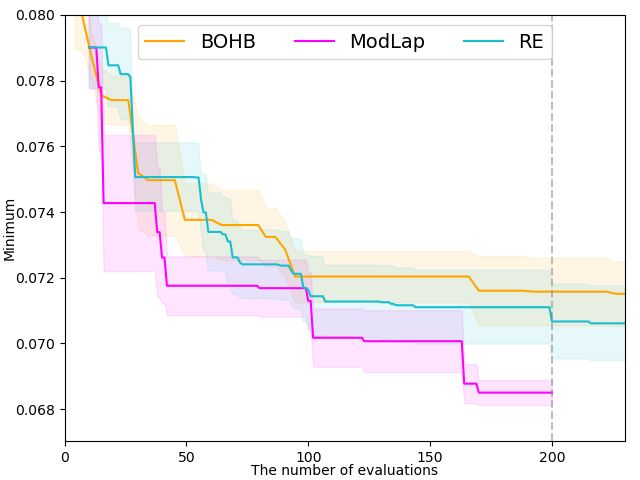
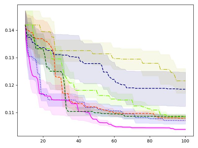
SMAC              TPE             ModDif            ModLap         CoCaBO-0.0      CoCaBO-0.5       CoCaBO-1.0
   Func2C +0.006 ± 0.039 −0.192 ± 0.005 −0.066 ± 0.046 −0.206 ± 0.000 −0.159 ± 0.013 −0.202 ± 0.002 −0.186 ± 0.009
   Func3C +0.119 ± 0.072 −0.407 ± 0.120 −0.098 ± 0.074 −0.722 ± 0.000 −0.673 ± 0.027 −0.720 ± 0.002 −0.714 ± 0.005
  Ackley5C +2.381 ± 0.165 +1.860 ± 0.125 +0.001 ± 0.000 +0.019 ± 0.006 +1.499 ± 0.201 +1.372 ± 0.211 +1.811 ± 0.217
                    Figure 2: Func2C(left), Func3C(middle), Ackley5C(right) (Mean±Std.Err. of 5 runs)
problems from Ru et al. [2020], 2 hyperparameter optimiza-             forms One-hot BO [authors, 2016] and EXP3BO [Gopaku-
tion problems (SVM [Smola and Kondor, 2003] and XG-                    mar et al., 2018]. For CoCaBO, we consider 3 variants using
Boost [Chen and Guestrin, 2016]) and the joint optimization            different mixture weights.9
of neural architecture and SGD hyperparameters.
As per our method, we consider M OD L AP which is of the               5.1     SYNTHETIC PROBLEMS
form Eq. 5 with the following frequency modulating func-
tion.                                                                  We test on 3 synthetic problems proposed in Ru et al.
                                              1                        [2020]10 . Each of the synthetic problems has the search
    fLap (λ , k c − c0 kθ |α, β ) =                         (9)
                                    1 + β λ + αk c − c0 k2θ            space as in Tab. 1. Details of synthetic problems can be
                                                                       found in Ru et al. [2020].
Moreover, to empirically demonstrate the importance of
the similarity measure behavior, we consider another kernel                                 Conti. Space      Num. of Cats.
following the form of Eq. 5 but disrespecting the frequency                     Func2C        [−1, 1]2              3, 5
modulation principle with the function                                          Func3C        [−1, 1]2             3, 5,4
                                                                               Ackley5C        [−1, 1]       17, 17, 17, 17, 17
  fDi f (λ , k c − c0 kθ |α, β ) = exp (−(1 + αk c − c0 k2θ )β λ )
                                                               (10)               Table 1: Synthetic Problem Search Spaces
We call the kernel constructed with this function M OD D IF.           On all 3 synthetic benchmarks, M OD L AP shows competitive
The implementation of these kernels is publicly available.4            performance (Fig. 2). On Func2C and Func3C, M OD L AP
In each round, after updating with an evaluation, we fit a GP          performs the best, while on Ackley5C M OD L AP is at the
surrogate model using marginal likelihood maximization                 second place, marginally further from the first. Notably,
with 10 random initialization until convergence [Rasmussen,            even on Func2C and Func3C, where M OD D IF underper-
2003]. We use the expected improvement (EI) acquisition                forms significantly, M OD L AP exhibits its competitiveness,
function [Donald, 1998] and optimize it by repeated al-                which empirically supports that the similarity measure be-
ternation of L-BFGS-B [Zhu et al., 1997] and hill climb-               havior plays an important role in the surrogate modeling in
ing [Skiena, 1998] until convergence. More details on the              Bayesian optimization. Note that TPE and CoCaBO have
experiments are provided in Supp. Sec. 4.                              much shorter wall-clock runtime.

Baselines For synthetic problems and hyperparameter
optimization problems below, baselines we consider5 are                5.2     HYPERPARAMETER OPTIMIZATION
SMAC6 [Hutter et al., 2011], TPE7 [Bergstra et al., 2011],                     PROBLEMS
and CoCaBO8 [Ru et al., 2020] which consistently outper-
                                                                       Now we consider a practical application of Bayesian opti-
    4 https://github.com/ChangYong-Oh/                                 mization over mixed variables. We take two machine learn-
FrequencyModulatedKernelBO                                                   9 Learningthe mixture weight is not supported in the imple-
   5 The methods [Daxberger et al., 2019, Nguyen et al., 2019]
                                                                       mentation, we did not include it. Moreover, as shown in Ru et al.
whose code has not been released are excluded.                         [2020], at least one of 3 variants usually performs better than
   6 https://github.com/automl/SMAC3                                   learning the mixture weight.
   7 http://hyperopt.github.io/hyperopt/                                  10 In the implementation provided by the authors, only Func2C
   8 https://github.com/rubinxin/CoCaBO_code                           and Func3C are supported. We implemented Ackley5C.
SVM Method XGBoost
4.759 ± .141 SMAC .1215 ± .0045
4.399 ± .163 TPE .1084 ± .0007
4.188 ± .001 ModDif .1071 ± .0013
4.186 ± .002 ModLap .1038 ± .0003
4.412 ± .170 CoCaBO-0.0 .1184 ± .0062
4.196 ± .004 CoCaBO-0.5 .1079 ± .0010
4.196 ± .004 CoCaBO-1.0 .1086 ± .0008
Figure 3: SVM(left), XGBoost(right) (Mean±Std.Err. of 5 runs)
ing algorithms, SVM [Smola and Kondor, 2003] and XG- With a stratified train:test(7:3) split, the model is trained
Boost [Chen and Guestrin, 2016] and optimize their hyper- with 50 rounds and the best test error over 50 rounds is the
parameters. objective of SVM hyperparameter optimization.
In Fig. 3, M OD L AP performs the best. On XGBoost hy-
SVM We optimize hyperparameters of NuSVR in scikit-
perparameter optimization, M OD L AP exhibits clear benefit
learn [Pedregosa et al., 2011]. We consider 3 categorical
compared to the baselines. Here, M OD D IF wins the second
hyperparameters and 3 continuous hyperparameters (Tab. 2)
place in both problems.
and for continuous hyperparameters we search over log10
transformed space of the range.
NuSVR param.11 Range Comparison to different kernel combinations In
kernel {linear, poly, RBF, sigmoid } Supp. Sec. 5, we also report the comparison with differ-
gamma {scale, auto } ent kernel combinations on all 3 synthetic problems and 2
shrinking {on, off } hyperparameter parameter optimization problems. We make
C [10−4 , 10] two observations. First, M OD D IF, which does not respect
tol [10−6 , 1] the similarity measure behavior, sometimes severely de-
nu [10−6 , 1] grades BO performance. Second, M OD L AP obtains equally
good final results and consistently finds the better solutions
Table 2: NuSVR hyperparameters faster than the kernel product. This can be clearly shown by
For each of 5 split of Boston housing dataset with comparing the area above the mean curve of BO runs using
train:test(7:3) ratio, NuSVR is fitted on the train set and different kernels. The area above the mean curve of BO
RMSE on the test set is computed. The average of 5 test using M OD L AP is larger than the are above the mean curve
RMSE is the objective. of BO using the kernel product. Moreover, the gap between
the area from M OD L AP and the area from kernel product
XGBoost We consider 1 ordinal, 3 categorical and 4 con- increases in problems with larger search spaces. Even on
tinuous hyperparameters (Tab. 3). the smallest search space, Func2C, M OD L AP lags behind
XGBoost param.12 Range the kernel product up to around 90th evaluation and outper-
forms after it. The benefit of M OD L AP modeling complex
max_depth {1, · · · , 10}
dependency among mixed variables is more prominent in
booster {gbtree, dart}
higher dimension problems.
grow_policy {depthwise, lossguide}
objective {multi:softmax, multi:softprob}
eta [10−6 , 1] Ablation study on regression tasks In addition to the
gamma [10−4 , 10] results on BO experiments, we compare FM kernels with
subsample [10−3 , 1] kernel addiition and kernel product on three regression tasks
lambda [0, 5] from UCI datasets (Supp. Sec. 6). In terms of negative
Table 3: XGBoost hyperparameters log-likelihood (NLL), which takes into account uncertainty,
ModLap performs the best in two out of three tasks. Even
For 3 continuous hyperparameters, eta, gamma and subsam- on the task which is conjectured to have a structure suitable
ple, we search over the log10 transformed space of the range. to kernel product, ModLap shows competitive performance.
11 https://scikit-learn.org/stable/modules/ Moreover, on regression tasks, the importance of the fre-
generated/sklearn.svm.NuSVR.html quency modulation principle is further reinforced. For full
12 https://xgboost.readthedocs.io/en/ NLL and RMSE comparison and detailed discussion, see
latest/parameter.html Supp. Sec. 6Method #Eval. Mean±Std.Err.
BOHB 200 7.158 × 10⁻² ±1.0303 × 10⁻³
BOHB 230 7.151 × 10⁻² ±9.8367 × 10⁻⁴
BOHB 600 6.941 × 10⁻² ±4.4320 × 10⁻⁴
RE 200 7.067 × 10⁻² ±1.1417 × 10⁻³
RE 230 7.061 × 10⁻² ±1.1329 × 10⁻³
RE 400 6.929 × 10⁻² ±6.4804 × 10⁻⁴
RE 600 6.879 × 10⁻² ±1.0039 × 10⁻³
M OD L AP 200 6.850 × 10⁻² ±3.7914 × 10⁻⁴
For the figure with all numbers above, see Supp. Sec. 5.
Figure 4: Joint optimization of the architecture and SGD hyperparameters (Mean±Std.Err. of 4 runs)
5.3 JOINT OPTIMIZATION OF NEURAL epochs. For further details on the setup and the baselines we
ARCHITECTURE AND SGD refer the reader to Supp. Sec. 4 and 5.
HYPERPARAMETERS
We present the results in Fig. 4. Since BOHB adaptively
chooses the budget (the number of epochs), BOHB is plotted
Next, we experiment with BO on mixed variables by op-
according to the budget consumption. For example, the y-
timizing continuous and discrete hyperparameters of neu-
axis value of BOHB on 100-th evaluation is the result of
ral networks. The space of discrete hyperparameters A is
BOHB having consumed 2,500 epochs (25 epochs × 100).
modified from the NASNet search space [Zoph and Le,
2016], which consists of 8,153,726,976 choices. The space We observe that M OD L AP finds the best architecture in
of continuous hyperparameters H comprises 6 continuous terms of accuracy and computational cost. What is more,
hyperparameters of the SGD with a learning rate sched- we observe that M OD L AP reaches the better solutions faster
uler: learning rate, momentum, weight decay, learning rate in terms of numbers of evaluations. Even though the time
reduction factor, 1st reduction point ratio and 2nd reduc- to evaluate a new hyperparameter is dominant, the time to
tion point ratio. A good neural architecture should both suggest a new hyperparameter in M OD L AP is not negligi-
achieve low errors and be computationally modest. Thus, ble in this case. Therefore, we also provide the comparison
we optimize the objective f (a, h) = errvalid (a, h) + 0.02 × with respect the wall-clock time. It is estimated that RE
FLOP(a)/ maxa0 ∈A FLOP(a0 ). To increase the separability and BOHB evaluate 230 hyperparameters while M OD L AP
among smaller values, we use log f (a, h) transformed val- evaluate 200 hyperparameters (Supp. Sec. 4). For the same
ues whenever model fitting is performed on evaluation data. estimated wall-clock time, M OD L AP(200) outperforms com-
The reported results are still the original non-transformed petitors(RE(230), BOHB(230)).
f (a, h).
In order to see how beneficial the sample efficiency of
We compare with two strong baselines. One is BO-FM is in comparison to the baselines, we perform a
BOHB [Falkner et al., 2018] which is an evaluation- stress test in which more evaluations are allowed for RE
cost-aware algorithm augmenting unstructured bandit and BOHB. We leave RE and BOHB for 600 evaluations.
approach [Li et al., 2017] with model-based guidance. Notably, M OD L AP with 200 evaluations outperforms both
Another is RE [Real et al., 2019] based on a genetic competitors with 600 evaluations (Fig. 4 and Supp.Sec. 5).
algorithm with a novel population selection strategy. We conclude that M OD L AP exhibits higher sample effi-
In Dong et al. [2021], on discrete-only spaces, these ciency than the baselines.
two outperform competitors including weight sharing
approaches such as DARTS [Liu et al., 2018], SETN [Dong
and Yang, 2019], ENAS [Pham et al., 2018] and etc. In the 6 CONCLUSION
experiment, for BOHB, we use the public implementation13
and for RE, we use our own implementation. We propose FM kernels to improve the sample efficiency of
For a given set of hyperparameters, with M OD L AP or RE, mixed variable Bayesian optimization.
the neural network is trained on FashionMNIST for 25 On the theoretical side, we provide and prove conditions
epochs while BOHB adaptively chooses the number of for FM kernels to be positive definite and to satisfy the
similarity measure behavior. Both conditions are not trivial
13 https://github.com/automl/HpBandSter due to the interactions between quantities on two disparatedomains, the spatial domain and the frequency domain. Xuanyi Dong, Lu Liu, Katarzyna Musial, and Bogdan
Gabrys. Nats-bench: Benchmarking nas algorithms for
On the empirical side, we validate the effect of the condi-
architecture topology and size. IEEE Transactions on
tions for FM kernels on multiple synthetic problems and
Pattern Analysis and Machine Intelligence, 2021.
realistic hyperparameter optimization problems. Further, we
successfully demonstrate the benefits of FM kernels com- Stefan Falkner, Aaron Klein, and Frank Hutter. Bohb: Ro-
pared to non-GP based Bayesian Optimization on a chal- bust and efficient hyperparameter optimization at scale.
lenging joint optimization of neural architectures and SGD In International Conference on Machine Learning, pages
hyperparameters. BO-FM outperforms its competitors, in- 1437–1446. PMLR, 2018.
cluding Regularized evolution, which requires three times
as many evaluations. Marcello Fiducioso, Sebastian Curi, Benedikt Schumacher,
We conclude that an effective modeling of dependencies Markus Gwerder, and Andreas Krause. Safe contextual
between different types of variables improves the sample bayesian optimization for sustainable room temperature
efficiency of BO. We believe the generality of the approach pid control tuning. In IJCAI, pages 5850–5856. AAAI
can have a wider impact on modeling dependencies between Press, 2019.
discrete variables and variables of arbitrary other types,
including continuous variables. Shivapratap Gopakumar, Sunil Gupta, Santu Rana,
Vu Nguyen, and Svetha Venkatesh. Algorithmic assur-
ance: An active approach to algorithmic testing using
References bayesian optimisation. In Proceedings of the 32nd Inter-
national Conference on Neural Information Processing
The GPyOpt authors. Gpyopt: A bayesian optimiza- Systems, pages 5470–5478, 2018.
tion framework in python. http://github.com/
SheffieldML/GPyOpt, 2016. David Haussler. Convolution kernels on discrete structures.
Technical report, Technical report, Department of Com-
Ricardo Baptista and Matthias Poloczek. Bayesian opti- puter Science, University of California . . . , 1999.
mization of combinatorial structures. In ICML, pages
462–471, 2018. Frank Hutter, Holger H Hoos, and Kevin Leyton-Brown. Se-
James S Bergstra, Rémi Bardenet, Yoshua Bengio, and quential model-based optimization for general algorithm
Balázs Kégl. Algorithms for hyper-parameter optimiza- configuration. In International conference on learning
tion. In NeurIPS, pages 2546–2554, 2011. and intelligent optimization, pages 507–523. Springer,
2011.
Tianqi Chen and Carlos Guestrin. Xgboost: A scalable
tree boosting system. In Proceedings of the 22nd acm Kirthevasan Kandasamy, Willie Neiswanger, Jeff Schneider,
sigkdd international conference on knowledge discovery Barnabas Poczos, and Eric P Xing. Neural architecture
and data mining, pages 785–794, 2016. search with bayesian optimisation and optimal transport.
In Advances in Neural Information Processing Systems,
Yutian Chen, Aja Huang, Ziyu Wang, Ioannis Antonoglou, pages 2016–2025, 2018.
Julian Schrittwieser, David Silver, and Nando de Fre-
itas. Bayesian optimization in alphago. arXiv preprint Risi Imre Kondor and John Lafferty. Diffusion kernels on
arXiv:1812.06855, 2018. graphs and other discrete structures. In ICML, 2002.
Erik Daxberger, Anastasia Makarova, Matteo Turchetta, and Ksenia Korovina, Sailun Xu, Kirthevasan Kandasamy,
Andreas Krause. Mixed-variable bayesian optimization. Willie Neiswanger, Barnabas Poczos, Jeff Schneider, and
arXiv preprint arXiv:1907.01329, 2019. Eric P Xing. Chembo: Bayesian optimization of small
organic molecules with synthesizable recommendations.
R Jones Donald. Efficient global optimization of expensive
arXiv preprint arXiv:1908.01425, 2019.
black-box function. J. Global Optim., 13:455–492, 1998.
Xuanyi Dong and Yi Yang. One-shot neural architecture Andreas Krause and Cheng S Ong. Contextual gaussian
search via self-evaluated template network. In Proceed- process bandit optimization. In NeurIPS, pages 2447–
ings of the IEEE/CVF International Conference on Com- 2455, 2011.
puter Vision, pages 3681–3690, 2019.
Lisha Li, Kevin Jamieson, Giulia DeSalvo, Afshin Ros-
Xuanyi Dong, Mingxing Tan, Adams Wei Yu, Daiyi Peng, tamizadeh, and Ameet Talwalkar. Hyperband: A novel
Bogdan Gabrys, and Quoc V Le. Autohas: Efficient bandit-based approach to hyperparameter optimization.
hyperparameter and architecture search. arXiv preprint The Journal of Machine Learning Research, 18(1):6765–
arXiv:2006.03656, 2020. 6816, 2017.Shuai Li, Baoxiang Wang, Shengyu Zhang, and Wei Chen. Yves-Laurent Kom Samo and Stephen Roberts. Generalized
Contextual combinatorial cascading bandits. In ICML, spectral kernels. arXiv preprint arXiv:1506.02236, 2015.
volume 16, pages 1245–1253, 2016.
Bernhard Scholkopf and Alexander J Smola. Learning
Hanxiao Liu, Karen Simonyan, and Yiming Yang. Darts: with kernels: support vector machines, regularization,
Differentiable architecture search. arXiv preprint optimization, and beyond. MIT press, 2001.
arXiv:1806.09055, 2018.
Bobak Shahriari, Kevin Swersky, Ziyu Wang, Ryan P
Dang Nguyen, Sunil Gupta, Santu Rana, Alistair Shilton, Adams, and Nando De Freitas. Taking the human out of
and Svetha Venkatesh. Bayesian optimization for cate- the loop: A review of bayesian optimization. Proceedings
gorical and category-specific continuous inputs. arXiv of the IEEE, 104(1):148–175, 2015.
preprint arXiv:1911.12473, 2019.
Steven S Skiena. The algorithm design manual: Text, vol-
ChangYong Oh, Efstratios Gavves, and Max Welling. Bock: ume 1. Springer Science & Business Media, 1998.
Bayesian optimization with cylindrical kernels. In ICML,
pages 3868–3877, 2018. Alexander J Smola and Risi Kondor. Kernels and regulariza-
tion on graphs. In Learning theory and kernel machines,
Changyong Oh, Jakub Tomczak, Efstratios Gavves, and Max pages 144–158. Springer, 2003.
Welling. Combinatorial bayesian optimization using the
graph cartesian product. In NeurIPS, pages 2910–2920, Jasper Snoek, Hugo Larochelle, and Ryan P Adams. Practi-
2019. cal bayesian optimization of machine learning algorithms.
In NeurIPS, pages 2951–2959, 2012.
Antonio Ortega, Pascal Frossard, Jelena Kovačević, José MF
Moura, and Pierre Vandergheynst. Graph signal process- Benjamin Solnik, Daniel Golovin, Greg Kochanski, John El-
ing: Overview, challenges, and applications. Proceedings liot Karro, Subhodeep Moitra, and D. Sculley. Bayesian
of the IEEE, 106(5):808–828, 2018. optimization for a better dessert. In Proceedings of the
2017 NIPS Workshop on Bayesian Optimization, Decem-
Fabian Pedregosa, Gaël Varoquaux, Alexandre Gramfort,
ber 9, 2017, Long Beach, USA, 2017. The workshop is
Vincent Michel, Bertrand Thirion, Olivier Grisel, Mathieu
BayesOpt 2017 NIPS Workshop on Bayesian Optimiza-
Blondel, Peter Prettenhofer, Ron Weiss, Vincent Dubourg,
tion December 9, 2017, Long Beach, USA.
et al. Scikit-learn: Machine learning in python. the Jour-
nal of machine Learning research, 12:2825–2830, 2011. Kevin Swersky, Jasper Snoek, and Ryan P Adams. Multi-
Hieu Pham, Melody Guan, Barret Zoph, Quoc Le, and Jeff task bayesian optimization. In NeurIPS, pages 2004–
Dean. Efficient neural architecture search via parame- 2012, 2013.
ters sharing. In International Conference on Machine Jean-Philippe Vert, Koji Tsuda, and Bernhard Schölkopf. A
Learning, pages 4095–4104. PMLR, 2018. primer on kernel methods. Kernel methods in computa-
Carl Edward Rasmussen. Gaussian processes in machine tional biology, 47:35–70, 2004.
learning. In Summer School on Machine Learning, pages
Andrew Wilson and Hannes Nickisch. Kernel interpolation
63–71. Springer, 2003.
for scalable structured gaussian processes (kiss-gp). In
Esteban Real, Alok Aggarwal, Yanping Huang, and Quoc V ICML, pages 1775–1784, 2015.
Le. Regularized evolution for image classifier architecture
Ciyou Zhu, Richard H Byrd, Peihuang Lu, and Jorge No-
search. In Proceedings of the aaai conference on artificial
cedal. Algorithm 778: L-bfgs-b: Fortran subroutines for
intelligence, volume 33, pages 4780–4789, 2019.
large-scale bound-constrained optimization. ACM Trans-
Sami Remes, Markus Heinonen, and Samuel Kaski. Non- actions on Mathematical Software (TOMS), 23(4):550–
stationary spectral kernels. In NeurIPS, pages 4642–4651, 560, 1997.
2017.
Barret Zoph and Quoc V Le. Neural architecture search with
Jean-Louis Reymond and Mahendra Awale. Exploring reinforcement learning. arXiv preprint arXiv:1611.01578,
chemical space for drug discovery using the chemical 2016.
universe database. ACS chemical neuroscience, 3(9):649–
657, 2012.
Binxin Ru, Ahsan Alvi, Vu Nguyen, Michael A Osborne,
and Stephen Roberts. Bayesian optimisation over multi-
ple continuous and categorical inputs. In International
Conference on Machine Learning, pages 8276–8285.
PMLR, 2020.You can also read