UNISWAP: Impermanent Loss and Risk Profile of a Liquidity Provider

UNISWAP: Impermanent Loss and Risk
 Profile of a Liquidity Provider
 Andreas A Aigner*, Gurvinder Dhaliwal+

 *
 TradeFlags, Vienna, Austria, +Fuel Ventures, London, United Kingdom

 Submitted: June 23, 2021, Updated: June 25, 2021

Uniswap is a decentralized exchange (DEX) and was first launched on November 2, 2018 on the Ethereum mainnet [1] and is part of
an Ecosystem of products in Decentralized Finance (DeFi). It replaces a traditional order book type of trading common on centralized
exchanges (CEX) with a deterministic model that swaps currencies (or tokens/assets) along a fixed price function determined by the
amount of currencies supplied by the liquidity providers. Liquidity providers can be regarded as investors in the decentralized
exchange and earn fixed commissions per trade. They lock up funds in liquidity pools for distinct pairs of currencies allowing market
participants to swap them using the fixed price function. Liquidity providers take on market risk as a liquidity provider in exchange for
earning commissions on each trade. Here we analyze the risk profile of a liquidity provider and the so called impermanent (unrealized)
loss in particular. We provide an improved version of the commonly denoted impermanent loss function for Uniswap v2 on the semi-
infinite domain. The differences between Uniswap v2 and v3 are also discussed.

Index Terms- Decentralized Finance, DeFi, Fintech, Automatic Market Maker, AMM, DEX, Decentralized Exchange,
Cryptocurrency, Uniswap, Ethereum, ERC-20, Yield farming, Liquidity Provider

JEL- A10, B10, D40, D47, D53, E44, F30, F60, G10, G14, G21, G23, G51, I10, K10, L14, M10, O16, O31, O33, O40, P10, C63,
C70, D83, D85.

 I. INTRODUCTION

D ecentralized Finance is a unique new application to the world of cryptos [2-41]. An easy introduction to this sector is found in
 [23] and [20]. It offers products and services akin to centralized finance but instead is decentralized. Meaning that where there
was a central authority handling all the transactions, there is none. Market participants interact directly with other participants through
the use of predefined contracts, smart contracts. There are also novel products that are unique to decentralized finance. Uniswap a
decentralized exchange with automated market making functionality is one example. Uniswap started off with offering exchanges
between Ethereum and other currencies (or tokens/assets) [1]. Version 2 generalized this to the exchange between any pair [42].
Liquidity providers of v2 provide liquidity on a semi-infinite domain of the exchange rate, whereas v3 allows liquidity providers to set
an arbitrary finite range instead, thereby maximizing the use of their pooled assets [43]. Uniswap uses a fixed price function, also
known as a liquidity function, to set the price for each trade. The function is called a market making function and the programmatic
use of this function to offer prices is commonly referred to as automated market making. It has its origins in prediction markets, online
ad auctions and instructor rating markets, where one of the most used scoring rule is the logarithmic market scoring rule (LMSR) [44,
45].
Historically market making has been studied widely [46-61], since it has its origin in the stock and forex market, where firms would
take the role of a designated market maker (DMM) on the exchange in return for being able to profit from the liquidity of the market.
With the advent of high frequency trading and algorithmic trading such automated means of trading can, in a sense, also be regarded
as automated market making. In the derivatives market the option market maker would be quoting bid-offer prices for options on a
whole range of stocks listed on an exchange in order to provide liquidity and collect premium and commissions in return [62, 63].
These methods are also referred to as algorithmic market making or quite often called automated market making as well. The
deterministic market making functions are normally not used in these situations, instead they are sophisticated stochastic models
acting as a feedback loop, responding elastically to market supply and demand.
The market making functions used in decentralized finance instead are deterministic. Of those that exist today there are several
different decentralized exchanges that use different market making functions and a number of papers have been written related to them
[44, 45, 64-89]. Some other examples are Bancor, Balancer, Curve, Sushiswap.
The reason why decentralized exchanges have turned to deterministic market making functions is because running a decentralized
exchange with an order book is simply unfeasible. The transactions would be slow and it would be very expensive to run. A
deterministic function can be easily coded in a smart contract on the Ethereum chain instead of replicating the dynamics of an order

UNISWAP: Impermanent Loss and Risk Profile of a Liquidity Provider
Aigner, Andreas A.
 2

book similar to a centralized exchange. The disadvantage of course is that the liquidity across the whole price domain is fixed too at
every time, provided there is no in or outflow of liquidity.
But an advantage a decentralized exchange has though is that it is decentralized, permissionless, secure, censorship-resistant and
automated, void of any third-party interaction [64]. It operates by various participants interacting directly with each other (through
smart contracts). It is secured by the Ethereum network that is designed to be hackproof. It is censorship resistant since participants
from anywhere in the world can interact with each other without the need for approval or KYC. It is automated in the sense that,
possibly except for the web interface/front end itself, it is extremely unlikely that the smart contracts will stop working. The
decentralized exchange will always be available 24/7.
A novel key advantage a decentralized exchange has to offer, is the fact that market participants can earn income on their balances, not
without any risks though. But it is important to highlight here that centralized exchanges or platforms such as Coinbase collect
enormous transactions fees (Coinbase Revenue 2020 was $1.27bn). Decentralized exchanges such as Uniswap offer market
participants a very attractive opportunity to earn such transaction fees. By depositing funds into a liquidity pool, they can earn on
every transaction. Market participants who use the exchange facility pay a fixed fee (0.05%, 0.3% or 1%) depending on the liquidity
pool and pair they want to trade. These fees are fixed and users know that these fees get paid directly to other market participants
being liquidity providers.
Considering the revenue of crypto exchange companies such as Coinbase, this offers up an alternative business model for crypto and a
potentially lucrative use case for crypto currencies in general.
Average returns for liquidity providers in the biggest liquidity pool on Uniswap make around 1% per week (52%pa) in return for the
last couple of weeks before the time of writing [90]. There are smaller liquidity pools with more illiquid currencies/tokens that can
have extreme average returns, but they don’t come without any serious risks involved (see recent case of Mark Cuban’s Titan-DAI
liquidity pool disaster [91, 92]).
Novel investors and curious crypto enthusiasts will want to get a firm grip on understanding exactly what the risks are in being a
liquidity provider. Here a detailed analysis of the risk profile is given, the paper is grouped into the following sections: Section II
describes the Market Making Function, Section III discusses Impermanent Loss and the Risk Profiles associated with Uniswap v2 and
v3 and Section IV concludes with a summary. Appendix I has a derivation of the impermanent loss and Appendix II is a guide on
How to become a Liquidity Provider.

 II. MARKET MAKING FUNCTION
The market making function that Uniswap v2 uses is the constant product function and can be described by this equation

 ∙ = Eq. (1)

where x and y are the amounts of each asset in the liquidity pool and K represents the total amount of liquidity. Furthermore, it is
required that the ratio of the two assets has to always represent the exchange rate of the two assets P.
 Eq. (2)
 = 
 
The relationship of x and y can be plotted as in Figure 1 where the exchange rate P goes to infinity for X large and Y small and
approaches zero for the opposite case. Each point along this curve therefore represents a predefined ratio of amounts x and y making
up the liquidity pool.

 Figure 1: Liquidity function of Uniswap v2.

UNISWAP: Impermanent Loss and Risk Profile of a Liquidity Provider
Aigner, Andreas A.
 3

If someone wants to purchase an amount of ∆ reducing the amount of liquidity in y, he will be quoted an amount of ∆ that exactly
matches the constraint given by the market making function. Both the current Price of the liquidity pool (x,y) and the new price of the
liquidity pool (x+∆ , − ∆ ) have to satisfy Eq. (1) such that the product of both is equal to the constant K. This means that we can
solve this equation
 ∙ = ( + ∆ ) ∙ ( − ∆ )

for ∆ 
 ∆ Eq. (3)
 ∆ = ∙ 
 − ∆ 

The amount of ∆ charged for every amount ∆ offered is therefore known and defined along the whole liquidity curve. We can
notice that the more asset x is depleted the higher the amount of ∆ is charged for a fixed amount of ∆ and likewise the more asset y
is depleted the higher the amount of ∆ is charged for a fixed amount of ∆ .

Furthermore, we note here that solving Eq. (1) and Eq. (2) for x and y we can express the liquidity reserves in terms of the Price P and
the constant K as
 / Eq. (4)
 = √ ∙ and = . 0

In Uniswap v3 the liquidity is limited to a range in prices ∈ 2 345 , 789: ; at which one of the liquidity amounts is zero at either end.
This means that when the price of the asset reaches the lower bound then all the assets are in asset y and when the price of the asset
reaches the upper bound all the assets are in asset x. This amounts to a shift in the liquidity function, Eq. (1), which can be expressed
as

 < ∙ < = Eq. (5)

where
 / Eq. (6)
 < = + = ∙ 345 and < = + .0
 >?@A

The intersections of this liquidity curve with the x and y axis is given by

 G G Eq. (7)
 = 0, CDE = √ ∙ F − K
 =0HIJ =0>?@A

and

 CDE = √ ∙ L= 789: − = 345 M, =0 Eq. (8)

 Figure 2: Liquidity function of Uniswap v3

UNISWAP: Impermanent Loss and Risk Profile of a Liquidity Provider
Aigner, Andreas A.
 4

corresponding to the points (0, CDE ) and ( CDE , 0) in Figure 2.

Each Price P in the range ∈ 2 345 , 789: ; corresponds to a pair of points ( , ) between (0, CDE ) and ( CDE , 0). Outside of this
range the liquidity pool consists solely of one of the assets x or y.

When we think of an order book market we think of a distribution of orders below and above the current market price (spot price), as
is sketched in Figure 3. The distribution of bid and offers might be symmetric or asymmetric. Bid-offers might be concentrated around
the spot price and fall off away from it, which is referred to as convex (higher spot liquidity), or increase with prices away from the
spot price (low spot liquidity), which is called concave. In the case of an automated market making, such as Uniswap, one can think of
the quantities available to trade at different bid offer prices as well and it will look something similar to what is shown in Figure 3.
The equivalent order book has increasing amounts of asset y the lower the price of y is with respect to x and less on offer the higher
the price of y is. The amounts can be thought of as bucketed and are represented by the amount of ∆ for each ∆ . This corresponds to
the tick sizes in the common stock market. While we might not have a symmetric order book around a current spot level, we do still
have an equivalent order book, which is not dynamic though and stays fixed as long as there is no in or outflow of liquidity.

 Figure 3: Examples of order books and market depth.

 III. IMPERMANENT LOSS & RISK PROFILE

Impermanent loss is the loss incurred by a market making position versus keeping the initially allocated amounts fixed. There are a
number of online calculators for the impermanent loss such as [93-96]. The Uniswap website also has a formula for it given here [97]
and there are a couple of papers and websites containing the same formula for it here [68, 98, 99]. The formula quoted there is
incorrect and will derive the correct impermanent loss equation here. Please note that the term impermanent loss can rather be thought
of as what is usually referred to as an unrealized loss. This is a more common way to call such a loss, which only becomes realized if
one chooses to sell out of a position which has dropped in value.

Given an initial Price N the value N of a 2-asset portfolio initially is given by

 N = + N ∙ Eq. (9)

The new value G when traded at a new price G is given by

 G = < + G ∙ < Eq. (10)

UNISWAP: Impermanent Loss and Risk Profile of a Liquidity Provider
Aigner, Andreas A.
 5

Compare this to a 2-asset portfolio with fixed quantities where the value initially would be the same as above, but the value at the new
price would also be given by

 + G ∙ Eq. (11)

The impermanent or unrealized loss is the difference between the portfolio change of the market making portfolio and the change in
value of a portfolio of assets with fixed quantities. This is the loss on top of a mark to market move of an equivalent fixed-quantity
portfolio.

It can be written as

 < + G ∙ < − ( + N ∙ ) − L + G ∙ − ( + N ∙ )M Eq. (12)

which simplifies to

 < − + G ∙ < − N ∙ − ( G − N ) ∙ Eq. (13)

Substitution and cancelling of terms yield the following equation for the impermanent loss 

 ∆ 1 Eq. (14)
 = = √ − ∙ ( + 1)
 N 2

 G
Which is expressed in terms of R, the ratio of the new versus the old price = V . A detailed derivation with all the steps involved
 N
is provided in Appendix I.

When we chart this and compare it to the calculations from the other sources we get a loss which is less pronounced for big drops, but
bigger for larger price moves, see Figure 4. When the price drops by 1/2 you have a loss −4.29% as compared to −5.72% . On the
contrary when the price increases by 2X you have a loss of −8.58% compared to a loss of −5.72% using the equation commonly
quoted. For a 2/3 drop this difference increases to −9.05% and 13.62%, versus −26.79% and 13.40%. The reason being is that the
impermanent loss equation commonly quoted is calculated relative to the final value of the portfolio. Here we calculate it versus the
initial value of the portfolio which makes more sense as an investor. Since looking at a PNL relative to the final PNL of a fixed
portfolio is misleading. Investors will always be surprised that their upside loss was higher than expected and their downside loss was
lower. It is particularly misleading when you are trying to compare different strategies with each other, since the final value of the
portfolio will be different for each strategy.

 Figure 4: Impermanent Loss

UNISWAP: Impermanent Loss and Risk Profile of a Liquidity Provider
Aigner, Andreas A.
 6

This is the impermanent loss on top of the mark to market of the initial position in assets x and y. If we want to know the total PNL we
have to include the mark to market of the initial position. Figure 5 shows a normalized version compared to a buy and hold with fixed
position sizes. A buy and hold portfolio has a linear relationship with its value since the value of the portfolio increases or decreases
with price linearly. The liquidity provider has a near linear relationship with price moves around the initial price only. When the price
drops to zero the portfolio value drops sharply to zero, since the liquidity provider is buying more and more of the asset losing its
value until the price is exactly zero and all of the other liquidity asset has dropped to zero. When the price increases the liquidity
provider loses more and more of the upside gains since he is selling more and more of the appreciating asset as the price increases.
This is the reason why the liquidity provider is losing money in both directions. He is buying the asset that is dropping in value and
selling the asset that is rising in value. Ideally the liquidity provider wants the asset prices to hover around his initial price, so one can
therefore think of the liquidity provider being ‘short volatility’ and ‘short convexity’. His position looks similar but is not identical to
someone being short a call and put option (a straddle). The risk profile here is nonlinear.

 Figure 5: Risk Profile of a Uniswap v2 liquidity provider and a Buy'n'Hold

The impermanent loss of Uniswap v3 can be calculated similarly to v2, first one needs to solve Eq. (5) and Eq. (6) for x and y,
similarly to Eq. (1),Eq. (2) and Eq. (4), which amounts to finding the roots of a quadratic equation in x and y.

 1 = 345
 ` + √ a + = 345 b ∙ + ∙ a − 1b = 0
 = 789: = 789:

and

 1 = 345 = 345
 ` + √ a + b∙ + ∙a − 1b = 0
 = 789: = 789:

Which can be solved using the ordinary p-q formula. Substituting this in the formula for the difference in the market to market move
of a 2-asset market making portfolio compared to a fixed quantity portfolio yields the impermanent loss of a Uniswap v3 liquidity
provider. We note from these quadratic equations that when 345 is zero and 789: is infinite we return the same equations as given
Eq. (4) in.

UNISWAP: Impermanent Loss and Risk Profile of a Liquidity Provider
Aigner, Andreas A.
 7

 Figure 6: Impermanent Loss of various Uniswap v3 liquidity positions and a Uniswap v2 liquidity position

Examples for various price ranges are shown in Figure 6 and compared to the impermanent loss of a Uniswap v2 liquidity provider. It
is obvious that when the fixed range of the liquidity provider approaches the semi-infinite domain of the v2 liquidity provider the
impermanent loss functions become similar. For smaller ranges the impermanent loss gets more symmetric and decreases around the
initial value having steeper losses than an ordinary Uniswap v2 position with a semi-infinite domain will have.

For example, when the price moves by 20% the impermanent loss of a v2 liquidity position will be −0.56% and −0.46% while a
fixed range of 25% and 125% of initial will have an impermanent loss of −4.75% and −3.8%. Some more examples are collected in
Table 1.

Table 1: Impermanent Loss of various Liquidity Positions

 %Move/Range -20% Initial 20%
 [0%, inf) -0.56% 0 -0.46%
 [0%, 200%] -0.86% 0 -0.70%
 [25%, 175%] -1.5% 0 -1.22%
 [50%, 150%] -2.34% 0 -1.91%
 [75%, 125%] -4.75% 0 -3.8%

Consider a fixed range of 80% and 120%, the risk profile of such a liquidity position will look like Figure 7. Since the liquidity
outside of this range is composed entirely of one or the other asset the value of the portfolio will decline linearly below the lower
bound, since the pool consists of 100% of the declining asset, and remain constant above the upper bound, since the pool consists of
100% of the asset that is not appreciating. Compare this to a buy and hold portfolio of the same initial asset distribution, which
increases/decreases linearly with price. Note that when the price drops to zero for one asset your buy and hold portfolio will still be
worth 50% whereas the market making portfolio will be have lost 100% of its value since it was long 100% of the declining asset
already since it breached the lower bound.

UNISWAP: Impermanent Loss and Risk Profile of a Liquidity Provider
Aigner, Andreas A.
 8

 Figure 7: Risk Profile of an 80%-120% liquidity position.

 Figure 8: Impermanent loss of an 80%-120% liquidity position.

Figure 8 shows the corresponding impermanent loss of a [80%, 120%] range liquidity provider. We note here that a liquidity provider
portfolio risk profile is always at a disadvantage to a buy and hold portfolio. Some websites interactive calculators erroneously show a
risk profile that indicate that you will lose less than a buy and hold portfolio. This is not the case. In essence as exhibited by the PNL
profile, Figure 7 and Figure 8, it is similar to being synthetically short variance (short Gamma) on the underlying, earning Theta
(yield). Extreme spot price moves will manifest this short gamma; in further papers we will discuss periodic delta hedging strategies
and short dated puts to ameliorate and subdue the risk characteristics endemic in the form of liquidity positions discussed in this paper.

 IV. CONCLUSION
Current investors can purchase crypto using centralized exchanges (CEX), which are companies in the conventional sense that provide
a platform or app to deposit fiat currencies into or offer the option to purchase using credit cards. They provide an on-ramp facility for
investors to exchange fiat currencies into crypto. Many of these platforms offer interest rates on crypto (and fiat) deposits and further
investment products such as locked staking.
In contrast to centralized exchanges there are decentralized exchanges (DEX) which have no central entity managing the deposits.
Instead the interactions between participants are handled by smart contracts on the Ethereum chain. Assets get exchanged using a
smart contract using a deterministic market making function that has a set price for every amount of token that gets offered or bid.
This function of liquidity represents a distribution of bid offers similar to order book type markets provided by centralized exchanges.
Instead of having a dynamic order book with market depth the depth of bid-offers is fixed, as long as the amount of liquidity

UNISWAP: Impermanent Loss and Risk Profile of a Liquidity Provider
Aigner, Andreas A.
 9

underlying doesn’t change. The liquidity in such a liquidity pool is not provided by a centralized entity, as would be the case on a
CEX, but instead by other individual market participants who get compensated by trade commissions in return for the risk they take
on. The risk that a liquidity provider takes on is essentially of two kinds. When setting up a position initially an amount of each asset
is provided and usually in a ratio of about 50% each. A liquidity provider therefore has, without any other interaction, a linear risk of
the price of one of the assets changing versus the other asset. This is normally called Delta risk, since Delta in the option market is the
rate of change of one asset with the change in the other asset. Usually the other asset in such case is the base currency such as the US
Dollar. When you have a liquidity position you can have two assets which are both different to your US Dollar, so in practice you
have Delta risk on both currencies already.
The second risk that a Liquidity Provider has is the change in his position due to other market participants interacting with his liquidity
pool. Every time part of his position gets bought or sold, the price of the asset changes. And at either one of the extreme ends of the
prices, albeit 0 and infinity or a fixed range ( 345 and 789: ) he will have swapped one of the assets into the other assets completely.
The difference between the value of the portfolio of two assets with and without these transactions is called impermanent loss. It can
also be called unrealized loss in this situation, because if the price of the asset reverses to the initial price a liquidity provider would
end up with exactly the same position as what he set out with, having zero loss, but would have earned commissions along the whole
price swing. The Delta risk above is also an unrealized loss, since the Liquidity provider ends up with zero loss or gain when the price
drops back to the same initial price.
To summarize both the Delta as well as the impermanent loss are unrealized as long as the liquidity provider does not withdraw his
liquidity from the pool. At the point where the liquidity provider withdraws his funds from the pool, is when his loss or gain due to the
impermanent loss gets realized. His loss or gain due to the Delta risk is only realized once he sells out of his position or swaps one of
the assets for the other.
Here we have described the underlying mechanics of a market making function in Section II, and have derived the impermanent loss
function for Uniswap v2 and v3, in Section III. We have provided an improved impermanent loss formula for the commonly quoted
Equation for v2 and online calculators for v3. We have charted the risk profile of positions in v2 and v3 and compared various
different ranges of liquidity, showing that v2 is approached in the limit of the range going to infinity.
Uniswap is one of the most liquid decentralized exchanges. There are other exchanges that offer similar market making products that
will work according to different market making functions. There is still ongoing research into these which can be found in our
references below.
What other risks exist for a liquidity provider? One of the key properties of a liquidity provider is that he is willing to own all of either
one of the assets at either his lower price limit or zero (in the case of v2). This means that when one of the assets has huge price
swings or is compromised, as for example in the recent case of Mark Cuban (ironfinance, Titan-DAI). The liquidity provider would
have sold all of his reliable assets to purchase the compromised asset. A liquidity provider cannot be certain that he will own any or
part of either asset at the time of redemption. If a liquidity provider is happy to own either one of the assets at its low and sell out of it
at a higher level, he will get compensated for this through the commissions he will earn when participants are trading on his liquidity
pool.
Since market making functions are using individual liquidity curves there are also various arbitrage opportunities. Some with external
order book type exchanges as well as internally between a trio of currency pairs that end up quoting different cross exchange rates for
the exchange rate in the first pair [72]. Provided the arbitrage opportunity is greater than the transaction costs required it will be
utilized. The work involved in taking advantage of these opportunities is extensive, especially if its across different exchanges. There
is however the advantage of using atomic transactions, meaning one smart contract transaction that will exercise a round trip in the
arbitrage. Building such arbitrage tools as a regular person will be too difficult, but suffice to say it is most certainly done already to
some extent. In fact decentralized exchanges such as Uniswap can represent a ‘fair’ price of assets since it will have been arbed
already, these are called price oracles and Uniswap is regarded as such as well [44] .
As of time of writing the biggest liquidity pool on Uniswap (ETH-USDC) is earning an average of 1.5% weekly [90, 100, 101], which
amounts to 78% annually at the current trading volumes. A liquidity provider who provides an equal amount of liquidity mapped
along the price curve can expect to earn the same or similar return.
There are other risks involved with crypto with have to do with smart contract risk, fraudulent DEXs, regulatory clampdowns, ISP
provider censorship and other exterior risks [102-106]. There are discussed widely in the literature here and here. Useful websites for
monitoring the Defi space and security issues are vfat.tools, RugDoctor and rekt.news.

 APPENDIX I: DERIVATION OF THE IMPERMANENT LOSS FUNCTION V2

We start off with the change in the Value of a portfolio of a liquidity provider versus the change of portfolio of a fixed-asset portfolio.

UNISWAP: Impermanent Loss and Risk Profile of a Liquidity Provider
Aigner, Andreas A.
 10

 G − N − L e8Efg − N M

Notice how we can cancel the N term and write

 < + G ∙ < − ( + G ∙ )

Substituting Equations 1,2 in Equation x gives

 = ∙ G + G ∙ h − i= ∙ N + G ∙ h j
 G N

When you expand this you get

 1 1
 √ ∙ L= G − = N M + √ G ∙ ih − h j
 G N

The initial value of the portfolio is

 N = + N ∙ = = ∙ N + N ∙ h = 2= ∙ N
 N

Dividing this by N we get

 √ ∙ L= G − = N M √ G 1 1
 + ∙ ih − h j
 2= ∙ N 2= ∙ N G N

Cancelling out the terms gives

 L= G − = N M G = N − = G 1 G 1 G G
 + ∙a b = ih − 1j + h ∙ i1 − h j
 2= N 2= N = N ∙ = G 2 N 2 N N

When we introduce the ratio of prices

 G
 =
 N

This can simply be written as

 1 1
 = L√ − 1M + √ L1 − √ M
 2 2

Which becomes

 1
 = √ − ∙ ( + 1)
 2

Comparing this to the commonly quoted impermanent loss function, where the change in value as relative to the final portfolio value
is calculated instead of the initial value, you would divide by e8Efg instead of N and get [97, 107-109]

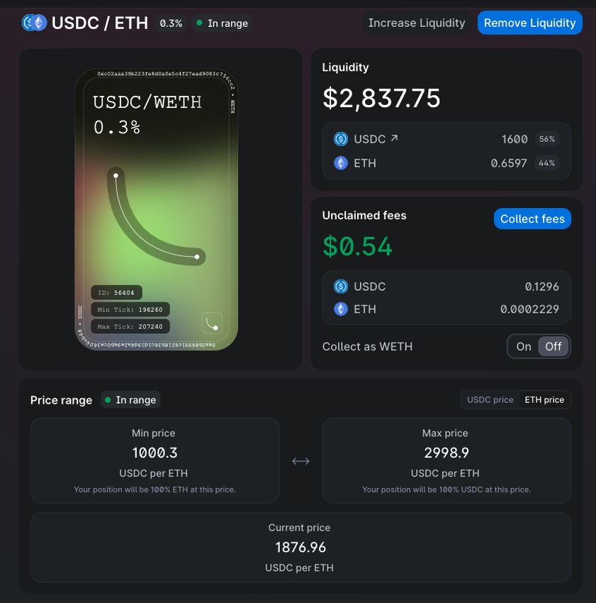
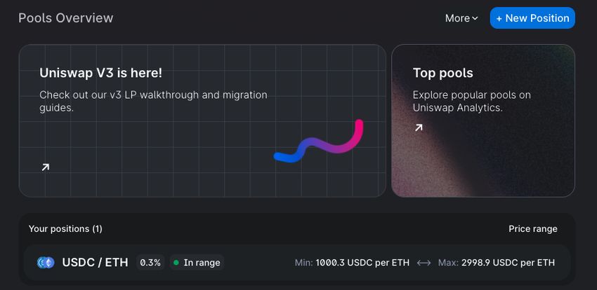
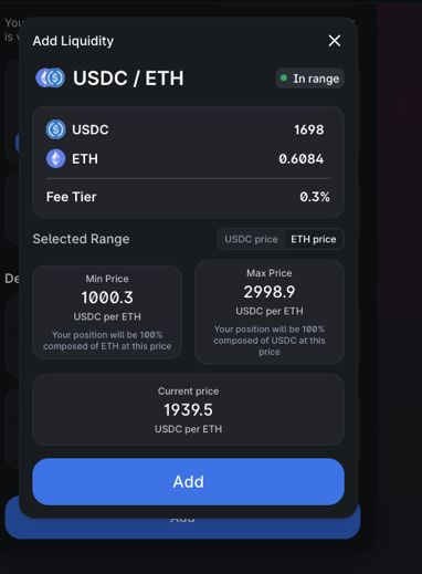
UNISWAP: Impermanent Loss and Risk Profile of a Liquidity Provider
Aigner, Andreas A.
 11

 2√ 
 = −1
 1+ 

 APPENDIX II: HOW TO BE A LIQUIDITY PROVIDER

We want to explain the steps involved and the fees involved in initiating a liquidity position. We choose the most liquid and biggest
liquidity pool on Uniswap which is ETH vs USDC. USDC is a stablecoin which is backed by US Dollar 1-1. The company which
issues these stablecoins is backed by investors such as Coinbase.

 1. First, we transfer by wire transfer or SEPA say 2000 USD to a centralized exchange for free.
 2. Then we buy 1000$ worth of ETH and incur a fee of say 0.00061814 ETH ($1.19 with ETHUSD = 1930$).
 3. We transfer this ETH to a wallet accepted by Uniswap and incur a fee of 6.98$ (0.0036ETH). We use Metamask.
 4. We purchase 1000$ worth of USDC for a fee of about $1.19.
 5. We also transfer this amount of USDC to the accepted wallet and incur a fee of 8$
 6. Connecting your wallet to Uniswap we find the most liquid pool using the charts. One of the options is to provide liquidity.
 Since all the liquidity pools have to use a wrapped ETH (WETH9) to provide liquidity we have to convert the ETH we have
 in our wallet to WETH9. We do this using Uniswap which incurs a 1.17$ fee.
 7. Now we can start with setting up the liquidity position. We choose to allocate all of the wrapped ETH (WETH9) and it will
 return us the required USDC we need to allocate. If the balance of ETH versus USDC is not exactly 50:50 then you will need
 to transfer for USDC from as described above. Alternatively start off with buying more of the assets or reducing the amount
 of ETH to deposit.
 8. In our example we end up having a balance of 58% versus 42% roughly.

 9. Then one confirms the wrapped ETH and USDC position which costs 1.41$ and 1.87$ in fees.
 10. After waiting for these two transactions to go through you can confirm the liquidity position as a whole, which costs 13.26$
 to mint.

 11. After paying this last fee after a couple of minutes have passed one will see the position listed under ‘your positions’ and can

UNISWAP: Impermanent Loss and Risk Profile of a Liquidity Provider
Aigner, Andreas A.
 12

 12. View the Ethereum Address of this position on the Ethereum chain using Etherscan. One can also view the running fees
 collected for the liquidity pool. Which in this case is already around 0.54$ in fees after about 1-2hrs online.

In the whole process we have spent 35,07 USD or in this example 1.25% of the total value of the portfolio, which is less than the
theoretical return in commissions in one week (1.5%).

 CONFLICT OF INTEREST
The authors have, up to the date of writing, no position in any market maker or DEX token, or any liquidity pool (like Uniswap,
PancakeSwap, Quickswap, Curve, etc.) whether directly or indirectly. The author has no crypto positions worth mentioning that could
be regarded as a conflict of interest.

 AUTHORS
Email: Andreas A. Aigner, andreas@tradeflags.com
 Gurvinder Dhaliwal, guv@fuel.ventures

 REFERENCES

1. Adams, H. Uniswap Birthday Blog - V0. 2019; Available from: https://medium.com/uniswap/uniswap-
 birthday-blog-v0-7a91f3f6a1ba.
2. Ademola, R., A Beginners Guide to Decentralized Finance. Everything You Need To Know About The
 DeFi. 2021. 52.
3. Kelly, B., The Bitcoin Big Bang. How Alternative Currencies Are About to Change the World. 2014:
 John Wiley & Sons. 240.
4. Scholl, H., BitCoin Investment Know How -Passive Primer Profits. 2021: Estalontech.

UNISWAP: Impermanent Loss and Risk Profile of a Liquidity Provider
Aigner, Andreas A.
 13

5. Chen, Y. and C. Bellavitis, Blockchain disruption and decentralized finance: The rise of decentralized
 business models. Journal of Business Venturing Insights, 2020. 13: p. e00151.
6. Wibbels, E., J.R.P.W.e. al, and F.P.S.i. Europe, Business cycles and the political economy of
 decentralized finance: lessons for fiscal federalism in the EU. Citeseer.
7. Yavin, O. and A.J. Reardon, The Cointelligence Guide to Decentralized Finance (DeFi). 2020:
 Cointelligence LTD. 85.
8. Berenzon, D. Constant Function Market Makers: DeFi’s “Zero to One” Innovation. 2020; Available
 from: https://medium.com/bollinger-investment-group/constant-function-market-makers-defis-zero-to-
 one-innovation-968f77022159.
9. Daniels, J., Cryptoassets. Why Bitcoin, Ethereum, And Polkadot Will Change The Future - Learn About
 Blockchain Technology, What Hard Money Is, Decentralized Finance, And Interoperability Between
 Different Chains. 2021. 216.
10. Lewis, R., The Cryptocurrency Revolution. Finance in the Age of Bitcoin, Blockchains and Tokens.
 2020: Kogan Page Publishers.
11. Tsai, W.T., et al. Decentralized Digital-Asset Exchanges: Issues and Evaluation. in 3rd International
 Conference on Smart BlockChain, SmartBlock 2020. 2020. Institute of Electrical and Electronics
 Engineers Inc.
12. Uhlmann, M., Decentralized Finance. How Financial Independence is Possible with Blockchain
 Technology. 2020. 90.
13. Brown, Z., Decentralized Finance (DeFi). A Basic Guide For Beginners. 2021: Independently
 Published. 40.
14. Zetzsche, D.A., D.W. Arner, and R.P. Buckley, Decentralized Finance (DeFi). 2020.
15. Popescu, A.-D., Decentralized Finance (DeFi)–The Lego of Finance. researchgate.net.
16. Chohan, U.W., Decentralized Finance (DeFi): An Emergent Alternative Financial Architecture. 2021.
17. Team, I., Decentralized Finance Explained. IntroBooks.
18. Leonhard, R., Decentralized Finance on the Ethereum Blockchain. 2019.
19. Chen, Y. and C. Bellavitis, Decentralized Finance: Blockchain Technology and the Quest for an Open
 Financial System. 2019.
20. Schär, F., Decentralized Finance: On Blockchain- and Smart Contract-Based Financial Markets.
 Review, 2021. 103(2).
21. Johnson, K.N., Decentralized Finance: Regulating Cryptocurrency Exchanges. 2021.
22. Gudgeon, L., et al. The Decentralized Financial Crisis. in 2020 Crypto Valley Conference on
 Blockchain Technology, CVCBT 2020. 2020. Institute of Electrical and Electronics Engineers Inc.
23. Harvey, C.R., A. Ramachandran, and J. Santoro, DeFi and the Future of Finance 2021.
24. Hubbard, K., DeFi for the Diaspora. Creating the Foundation to a More Equitable and Sustainable
 Global Black Economy Through Decentralized Finance. 2021: Cagechain Media Group, LLC. 124.
25. Kiong, D.L.V., DEFI Guidebook. A Basic Guide to Decentralized Finance for Beginners. 2021:
 Independently Published. 514.
26. Tapscott, D. and A. Tapscott, Die Blockchain-Revolution. Wie die Technologie hinter Bitcoin nicht nur
 das Finanzsystem, sondern die ganze Welt verändert. 2016: Plassen Verlag. 450.
27. Hines, B., Digital Finance. Security Tokens and Unlocking the Real Potential of Blockchain. 2020: John
 Wiley & Sons. 208.
28. Finematics, How do LIQUIDITY POOLS work? (Uniswap, Curve, Balancer) | DEFI Explained. 2020. p.
 https://www.youtube.com/watch?v=cizLhxSKrAc.
29. Lau, D., D. Lau, and S.J. Teh, How to DeFi. 2020. 204.
30. Jensen, J.R., V. von Wachter, and O. Ross, An Introduction to Decentralized Finance (DeFi). Complex
 Systems Informatics and Modeling Quarterly (CSIMQ), 2021(26): p. 46-54.
31. Jensen, J.R. and O. Ross, Managing risk in DeFi. 2020.
32. Lantz, L. and D. Cawrey, Mastering Blockchain. 2020: O'Reilly Media. 284.

UNISWAP: Impermanent Loss and Risk Profile of a Liquidity Provider
Aigner, Andreas A.
 14

33. Hatcher, P., Modern Day Passive Income. From Flipping Websites to Decentralized Finance, Make
 Money No Matter How Automated the World Gets. 2021: Independently Published. 378.
34. Fiona, M., Notebook Planner Defi Decentralized Finance Ethereum. Cute, Finance, Over 100 Pages,
 Daily, Monthly, Work List, Simple, 6x9 Inch. 2020. 114.
35. Ramos, D. and G.Z.A.a.h.w.m. com, A Review of Decentralized Finance as an Application of Increasing
 Importance of Blockchain Technology. urano.io.
36. Werner, S.M., et al., SoK: Decentralized Finance (DeFi). 2021.
37. Wahrstätter, A., Stablecoin Billionaires - A Descriptive Analysis of the Ethereum-based Stablecoin
 Ecosystem. 2020.
38. Klages-Mundt, A., et al. Stablecoins 2.0: Economic Foundations and Risk-based Models. in 2nd ACM
 Conference on Advances in Financial Technologies, AFT 2020. 2020. Association for Computing
 Machinery, Inc.
39. Metwaly, A.H.W., Stake Hodler Capitalism. Blockchain and DeFi (Decentralized Finance). 2021. 152.
40. Lo, Y. and F. Medda, Uniswap and the Rise of the Decentralized Exchange 2020.
41. Harwick, C. and J. Caton, What’s holding back blockchain finance? On the possibility of decentralized
 autonomous finance. The Quarterly Review of Economics and Finance, 2020.
42. Adams, H., N. Zinsmeister, and D. Robinson, Uniswap v2 Core. 2020.
43. Adams, H., et al., Uniswap v3 Core, Uniswap.org, Editor. 2021.
44. Angeris, G. and T. Chitra, Improved Price Oracles: Constant Function Market Makers. 2020, Cornell
 University Library, arXiv.org: Ithaca.
45. Wang, Y., Automated Market Makers for Decentralized Finance (DeFi). 2020.
46. Sandås, P., Adverse selection and competitive market making: Empirical evidence from a limit order
 market. academic.oup.com.
47. Othman, A., Automated Market Making: Theory and Practice, in School of Computer Science. 2012,
 Carnegie Mellon University: Pittsburgh, PA 15213.
48. Amihud, Y. and H. Mendelson, Dealership market: Market-making with inventory. Journal of Financial
 Economics, 1980. 8(1): p. 31-53.
49. Guéant, O., C.A. Lehalle, and J.F.-T.M.a. financial, Dealing with the inventory risk: a solution to the
 market making problem. Springer.
50. Guéant, O., The Financial Mathematics of Market Liquidity: From optimal execution to market making.
 2016.
51. Guéant, O., Optimal market making. Applied Mathematical Finance, 2017.
52. Bradfield, J., A formal dynamic model of market making. JSTOR.
53. Chari, A., Heterogeneous Market-Making in Foreign Exchange Markets: Evidence from Individual
 Bank Responses to Central Bank Interventions. Journal of Money, Credit and Banking, 2007. 39(5): p.
 1131-1162.
54. Holden, C., Index arbitrage as cross-sectional market making. search.proquest.com.
55. Chakraborty, T. and M. Kearns, Market making and mean reversion.
56. Niederhoffer, V. and M.F.M. Osborne, Market Making and Reversal on the Stock Exchange. Journal of
 the American Statistical Association, 2012.
57. Spulber, D.F., Market making by price-setting firms. academic.oup.com.
58. Liu, H. and Y. Wang, Market making with asymmetric information and inventory risk. Journal of
 Economic Theory, 2016. 163: p. 73-109.
59. Toke, I.M., “Market Making” in an Order Book Model and Its Impact on the Spread, in Econophysics
 of Order-driven Markets. 2011, Springer, Milano. p. 49-64.
60. O'Hara, M., G.S.O.J.o.F. analysis, and Quantitative, The microeconomics of market making. JSTOR.
61. Madrigal, V. and J.A. Scheinkman, Price Crashes, Information Aggregation, and Market-Making.
 Journal of Economic Theory, 1997. 75(1): p. 16-63.

UNISWAP: Impermanent Loss and Risk Profile of a Liquidity Provider
Aigner, Andreas A.
 15

62. Jameson, M.E.L. and W. Wilhelm, Market Making in the Options Markets and the Costs of Discrete
 Hedge Rebalancing. The Journal of Finance, 1992. 47(2): p. 765-779.
63. Stoikov, S. and M.S.R.o.D. Research, Option market making under inventory risk. Springer.
64. Das, S. and M.M.-I. Nips, Adapting to a Market Shock: Optimal Sequential Market-Making. Citeseer.
65. Angeris, G., et al., An analysis of Uniswap markets. 2021, Cornell University Library, arXiv.org: Ithaca.
66. Tefagh, M., et al. Atomic bonded cross-chain debt. in 3rd International Conference on Blockchain
 Technology and Applications, ICBTA 2020. 2020. Association for Computing Machinery.
67. Mohan, V., Automated Market Makers and Decentralized Exchanges: a DeFi Primer 2020.
68. Wang, Y., L. Heimbach, and R. Wattenhofer, Behavior of Liquidity Providers in Decentralized
 Exchanges. arXiv.org, 2021. q-fin.CP.
69. Hickey, L. and M. Harrigan. The Bisq DAO: On the Privacy Cost of Participation. in 2020 IEEE
 Symposium on Computers and Communications, ISCC 2020. 2020. Institute of Electrical and
 Electronics Engineers Inc.
70. Park, A., The Conceptual Flaws of Constant Product Automated Market Making. 2021.
71. Angeris, G. and T. Chitra, Constant Function Market Makers. 2020.
72. Wang, Y., et al., Cyclic Arbitrage in Decentralized Exchange Markets. arXiv.org, 2021. q-fin.TR.
73. Zhang, Y., X. Chen, and D. Park, Formal Specification of Constant Product Market Maker Model and
 Implementation. 2018.
74. Zargham, M., J. Shorish, and K. Paruch. From Curved Bonding to Configuration Spaces. in 2nd IEEE
 International Conference on Blockchain and Cryptocurrency, ICBC 2020. 2020. Institute of Electrical
 and Electronics Engineers Inc.
75. Tassy, M. and D. White, Growth Rate of a Liquidity Provider’s Wealth in XY=c Automated Market
 Makers. 2020.
76. Zhou, L., et al., High-Frequency Trading on Decentralized On-Chain Exchanges. arXiv.org, 2020.
 cs.CR.
77. Buterin, V. Improving front running resistance of x*y=k market makers. 2018; Available from:
 https://ethresear.ch/t/improving-front-running-resistance-of-x-y-k-market-makers/1281.
78. Perez, D., et al., Liquidations: DeFi on a Knife-edge. 2020.
79. Evans, A., Liquidity Provider Returns in Geometric Mean Markets. arXiv.org, 2020. q-fin.MF.
80. Noyes, C., Liquidity Provider Wealth. 2020.
81. Bartoletti, M., J.H.-y. Chiang, and A. Lluch-Lafuente, Maximizing Extractable Value from Automated
 Market Makers. arXiv.org, 2021. cs.CR.
82. Tien, S.K., et al. Maximizing the Time Value of Cryptocurrency in Smart Contracts with Decentralized
 Money Markets. in 3rd IEEE International Conference on Blockchain, Blockchain 2020. 2020. Institute
 of Electrical and Electronics Engineers Inc.
83. Fritsch, R. and R. Wattenhofer, A Note on Optimal Fees for Constant Function Market Makers.
 arXiv.org, 2021. cs.GT.
84. Angeris, G., A. Evans, and T. Chitra, A Note on Privacy in Constant Function Market Makers. 2021,
 Cornell University Library, arXiv.org: Ithaca.
85. Buterin, V. On Path Independence. 2017; Available from:
 https://vitalik.ca/general/2017/06/22/marketmakers.html.
86. An optimization-based framework for automated market-making.
87. Yoo, Y., D. Seo, and M. Kim, Payment guaranteed polynomial exchange rate scheme and its
 application to cryptocurrency swaps. Annals of Emerging Technologies in Computing, 2020. 4(1): p.
 28-43.
88. Mazanec, J., Portfolio Optimalization on Digital Currency Market. Journal of Risk and Financial
 Management, 2021. 14(4): p. 160.
89. Angeris, G., A. Evans, and T. Chitra, When does the tail wag the dog? Curvature and market making.
 2020, Cornell University Library, arXiv.org: Ithaca.

UNISWAP: Impermanent Loss and Risk Profile of a Liquidity Provider
Aigner, Andreas A.
 16

90. @gammastrategies. Uniswap v3 Volume and Fees Collected. Available from:
 https://duneanalytics.com/gammastrategies/Uniswap-v3-Volume-and-Fees-Collected.
91. Even billionaire Mark Cuban is feeling the heat of the crypto crash. Available from:
 https://fortune.com/2021/06/17/crypto-titan-token-crash-mark-cuban/.
92. Mark Cuban Calls for Stablecoin Regulation After Trading Token That Crashed to Zero. Available
 from: https://www.bloomberg.com/news/articles/2021-06-17/mark-cuban-defi-iron-finance-crashed-
 100.
93. DecentYields. Impermanent Loss Calculator. Available from: https://decentyields.com/impermanent-
 loss-calculator.
94. Defi-lab.xyz. Impermanent Loss Calculator. Available from: https://defi-lab.xyz/uniswapv3simulator.
95. Defiyield. Impermanent Loss Calculator. Available from: https://safe.defiyield.app/advanced-
 impermanent-loss-calculator.
96. Vercel. Impermanent Loss Calculator. Available from: https://uniswap-simulator.vercel.app.
97. Uniswap.org. Impermanent Loss. Available from: https://uniswap.org/docs/v2/advanced-
 topics/understanding-returns/.
98. Pintail. Uniswap: A Good Deal for Liquidity Providers. 2019; Available from:
 https://pintail.medium.com/uniswap-a-good-deal-for-liquidity-providers-104c0b6816f2.
99. Krishnamachari, B., Q. Feng, and E. Grippo, Dynamic Curves for Decentralized Autonomous
 Cryptocurrency Exchanges. arXiv.org, 2021. q-fin.TR.
100. White, D. Uniswap’s Financial Alchemy. 2020; Available from:
 https://research.paradigm.xyz/uniswaps-alchemy.
101. White, D., Uniswap’s Financial Alchemy (Code). 2020.
102. Torres, C.F., et al., The Eye of Horus: Spotting and Analyzing Attacks on Ethereum Smart Contracts.
 arXiv.org, 2021. cs.CR.
103. Daian, P., et al. Flash boys 2.0: Frontrunning in decentralized exchanges, miner extractable value, and
 consensus instability. in 41st IEEE Symposium on Security and Privacy, SP 2020. 2020. Institute of
 Electrical and Electronics Engineers Inc.
104. Zhang, P., F. Xiao, and X. Luo. A Framework and DataSet for Bugs in Ethereum Smart Contracts. in
 36th IEEE International Conference on Software Maintenance and Evolution, ICSME 2020. 2020.
 Institute of Electrical and Electronics Engineers Inc.
105. Xu, J., et al., SoK: Decentralized Exchanges (DEX) with Automated Market Maker (AMM) protocols.
 arXiv.org, 2021. q-fin.TR.
106. Uniswap v3 Audit.
107. Erins, P. How to calculate Impermanent Loss: full derivation. 2021; Available from:
 https://medium.com/auditless/how-to-calculate-impermanent-loss-full-derivation-803e8b2497b7.
108. Martin, C. Understanding Returns. 2020 22 Dec 2020; Available from:
 https://uniswap.org/docs/v2/advanced-topics/understanding-returns/.
109. Pintail. Understanding Uniswap Returns. 2019; Available from:
 https://pintail.medium.com/understanding-uniswap-returns-cc593f3499ef.