This manuscript has been submitted for publication in GEOLOGY. Please note that the manuscript has not undergone peer-review. Subsequent versions ...
←
→
Page content transcription
If your browser does not render page correctly, please read the page content below
This manuscript has been submitted for publication in GEOLOGY. Please note that the
manuscript has not undergone peer-review. Subsequent versions of the manuscript may have
 slightly different content. If accepted, the final version will be available via the DOI link.
                        Please feel free to contact any of the authors.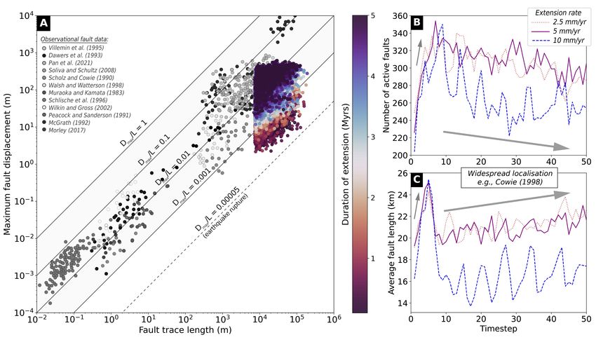
1    Bridging spatiotemporal scales of normal fault growth using

2    numerical models of continental extension

3    Sophie Pan1, John Naliboff2, Rebecca Bell1 and Chris Jackson3

4

     1
5        Earth Science and Engineering, Imperial College, Prince Consort Road, London, SW7 2BP, UK

     2
6        Department of Earth and Environmental Science, New Mexico Institute of Mining and

7    Technology, NM, USA

     3
8        Department of Earth and Environmental Sciences, The University of Manchester, Williamson

9    Building, Oxford Road, Manchester, M13 9PL, UK

10

11   ABSTRACT

12             Continental extension is accommodated by the development of kilometre-scale normal

13   faults, which grow by accumulating metre-scale earthquake slip over millions of years.

14   Reconstructing the entire lifespan of a fault remains challenging due to a lack of observational

15   data of appropriate scale, particularly over intermediate timescales (104-106 yrs). Using 3D

16   numerical simulations of continental extension and novel automated image processing, we

17   examine key factors controlling the growth of very large faults over their entire lifetime.

18   Modelled faults quantitatively show key geometric and kinematic similarities with natural fault

19   populations, with early faults (i.e., those formed within ca. 100 kyrs of extension) exhibiting

20   scaling ratios consistent with those characterising individual earthquake ruptures on active faults.
21   Our models also show that while finite lengths are rapidly established (< 100 kyrs), active

22   deformation is highly transient, migrating both along- and across-strike. Competing stress

23   interactions determine the overall distribution of active strain, which oscillates locally between

24   localised and continuous slip, to distributed and segmented slip. These findings demonstrate that

25   our understanding of fault growth and the related occurrence of earthquakes is more complex

26   than that currently inferred from observing finite displacement patterns on now-inactive

27   structures, which only provide a spatial- and time-averaged picture of fault kinematics and

28   related geohazard.

29

30

31   INTRODUCTION

32          Recent advancements in geodetic measurements allow for high-resolution surface

33   observations of crustal deformation (e.g., Elliott et al., 2016). Seismological and geodetic data

34   from a particular earthquake are inverted using modelled fault geometry to infer slip distribution

35   and magnitude (e.g., Wilkinson et al., 2015; Walters et al., 2018). These data show that

36   individual earthquake rupture patterns are variable and complex, with events typically temporally

37   and spatially clustered (e.g., Coppersmith, 1989; Nicol et al., 2006). Rupture lengths are often

38   considerably shorter than finite fault lengths, and multiple segment ruptures during a single event

39   can trigger surprisingly high-magnitude, hazardous earthquakes (7.9 Mw Kaikoura, New

40   Zealand; Hamling et al., 2017; 7.2 Mw El Mayor-Cucapah, Mexico; Fletcher et al., 2014) that

41   have recently challenged seismic hazard assessments (Field et al., 2014).
42          Large (e.g., tens of kilometres long, several kilometres of displacement) normal faults

43   grow by accumulating m-scale slip during earthquakes. In contrast to the short-time complexity

44   captured by seismological and geodetic data, 3D seismic reflection and field data show that slip

45   rates can be stable over substantially longer timescales (i.e., >106 yrs), incorporating potentially

46   thousands of seismic cycles distributed over millions of years. These data reveal that fault

47   displacement (i.e., cumulative slip) may simultaneously increase with length (the ‘propagating’

48   model; Walsh and Watterson, 1988), or accumulate on faults of near-constant length (the

49   ‘constant-length’ model; Walsh et al., 2002; Rotevatn et al., 2019; Pan et al., 2021). It is

50   challenging to reconstruct fault growth over shorter timescales (
64 Here, we use high-resolution (
86   inheritance observed in natural systems, where deformation exploits inherited weaknesses such

 87   as pre-existing faults (e.g., Phillips et al., 2016) or the margins of strong zones (e.g., ancient

 88   cratons; e.g., Dunbar and Sawyer, 1989).

 89           The 3D model results are analysed on a horizontal plane located 5 km below the initial

 90   model surface. To quantitatively analyse the geometry and kinematics of faults, fault

 91   identification and extraction is required (Fig. 1). We employ a Python workflow based on the

 92   spatial vertical derivative of the active deformation field (Supplementary Fig. 2), which

 93   effectively extracts localised, clustered regions of strain (i.e., relatively steep gradients of strain-

 94   profiles). This novel approach successfully recovers detailed interactions between distinct active

 95   fault strands without manual input across multiple timesteps. See the Supplemental Material for

 96   full details of our forward modelling and fault extraction approach.

 97

 98   MODELS PRODUCE REALISTIC FAULT PATTERNS

 99           Our model results show that in the final stages of rifting, the strain rate magnitude (Fig.

100   1A-C) and extracted active fault locations (Fig. 1D-F) for models with extension rates of 2.5, 5,

101   or 10 mm yr-1 reveal active deformation accommodated along complex fault networks. In models

102   with faster extension rates, the overall magnitude of strain rate increases and is accommodated

103   across increasingly diffuse zones of deformation (Fig. 1A-C). These networks contain faults of

104   varying lengths (c. 5-120 km), which often contain along-strike changes in strike, and that may

105   splay and link with adjacent structures. This complexity reflects both the randomisation of the

106   initial plastic strain field and the mechanical and kinematic interaction between adjacent faults.
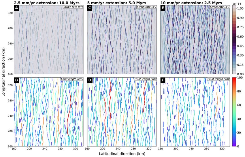
107   Overall, the fault network is geometrically similar, based on displacement-length (D-L) scaling

108   relationships, to those identified in natural systems (Fig. 2) (e.g., Walsh and Watterson, 1991).

109

110   FAULT PATTERNS ARE RAPIDLY ESTABLISHED

111          During the earliest stages of rifting, i.e., within the first resolvable timestep (c. 200, 100

112   and 50 kyrs for extension rates of 2.5, 5, or 10 mm yr-1, respectively), active deformation is

113   accommodated along distributed fault networks (Supplementary Video 1, 2) that are similar in

114   appearance to their finite fault patterns (Fig. 1). During the earliest timestep (< 100 kyrs) the

115   faults are seemingly under-displaced compared to geological D-L datasets, instead plotting close

116   to the slip-length ratio associated with individual earthquakes (c = 0.00005; see Wells and

117   Coppersmith, 1994 and Fig. 2A).

118          As near-maximum finite fault lengths are established from the onset of extension, faults

119   therefore predominantly accumulate displacement and move upwards in D-L space, behaviour

120   consistent with the constant-length fault growth model (e.g., Walsh et al., 2002; Rotevatn et al.,

121   2019; Pan et al., 2021). Our results show that fault lengths are established an order of magnitude

122   (
129   the structural level of observation. This is important, given it is deformation of the Earth’s

130   surface, and resulting thickness and facies changes in associated growth strata, that are typically

131   used to constrain normal fault kinematics (Jackson et al., 2017). The stratigraphic record may

132   therefore not record the earliest phase of extension leading to an erroneous assessment of

133   existing fault growth models and the timing of rift initiation and duration.

134

135   STRAIN ACCUMULATION REVEALS TRANSIENT BEHAVIOUR

136          Distinguishing between currently debated fault growth models has direct implications for

137   the nature of earthquake slip and potential moment magnitude, i.e., the ‘propagating’ model is

138   said to require a progressive temporal increase in the maximum earthquake magnitude, whereas

139   the constant-length model may be associated with constant slip rates and invariant earthquake

140   magnitude and recurrence (Nicol et al., 2005). Whereas our results demonstrate that finite

141   lengths were rapidly established (i.e., ‘constant-length’ model), they do not explicitly support

142   either of the two slip models, instead showing that active deformation is temporally and spatially

143   variable (i.e., earthquake slip is variable, not uniform), an observation consistent with slip

144   patterns characterising active fault networks (e.g., Friedrich et al., 2003; Oskin et al., 2007) and

145   analogue models (e.g., Schlagenhauf, 2008)

146          Time-series of the total number of active faults (Fig. 2B) and the average fault length in a

147   given population (Fig. 2C) reveal significant fluctuations throughout time. All three models (with

148   extensions rates of 2.5, 5, 10 mm yr-1) initiate with an increase in fault number and average fault

149   length (Fig. 2B, C), corresponding to an initially diffuse distributed pattern from the first

150   timestep that rapidly localises (i.e., reduces in deformation width) within the first c. 10 timesteps
151   (see Supplementary Videos 1-2, 4-6). Both fault number and mean length continue to fluctuate

152   throughout the remainder of extension, reflecting oscillations between localised and distributed

153   active deformation throughout the crust (Fig 2B, C). This behaviour is consistent with

154   spatiotemporal clustering of earthquakes promoted by stress interactions between neighbouring

155   faults (Stein 1999). Although transient behaviour continues for the remainder of extension, the

156   overall number of faults slowly decreases, and the average fault length slightly increases (Fig 2B,

157   C), demonstrating that large-scale localisation occurs as strain is concentrated onto fewer, larger

158   fault systems (e.g., Cowie, 1998).

159           Transient deformation occurs both along- and perpendicular to strike, which we view in a

160   regional model subset (Supplementary Video 4-6). Along-strike migration of deformation, which

161   we observe by summing longitudinally across the regional subset (Supplementary Video 7), is

162   consistent with the preferential propagation direction of rupture. The across-strike strain

163   migration correlates to along-strike bends, supporting observations from active settings that

164   earthquakes occur at segment boundaries (DuRoss et al., 2016), and that relays may be

165   associated with throw rate enhancements (Faure-Walker et al., 2009; Iezzi et al., 2018). Overall,

166   along- and across- strain migration, reflective of competing stress-interactions between faults in

167   the near field (e.g., Cowie, 1998) as documented in Fig. 2B and C, produce end-member

168   behaviours characterised by localised, continuous slip (Fig. 3A-C) and distributed, segmented

169   slip (Fig. 3D-F). This transient behaviour evolves without explicitly modelling the earthquake

170   cycle via a rate or rate-state friction type rheology (e.g., Dinther et al., 2013), suggesting that the

171   recurrence of large, clustered slip (e.g., Fig. 3A) can be mechanically underpinned by far-field,

172   dynamic triggering i.e., constant rates of tectonic extension.
173           The short-term variability and long-term stability of strain accumulation on the modelled

174   fault networks may be reconciled by considering how deformation is aggregated, both spatially

175   and temporally. As deformation is longitudinally summed across (latitudinally) increasing

176   regions, the strain rate profile becomes increasingly uniform as strain deficits in one location is

177   compensated for by increased strain in other, across-strike locations (Supplementary Video 7).

178   This reflects the coherence of faults at spatial scales larger than the individual fault surface (e.g.,

179   Nicol et al., 2006). Small-scale, distributed deformation in the form of near-fault drag accounted

180   for 30% greater geodetic slip rates (Oskin 2007). We suspect this value could be higher if the

181   spatial scale of observation increases to accommodate all distributed deformation, particularly at

182   higher extension rates (10 mm yr-1) where distributed deformation is relatively widespread (e.g.,

183   Fig. 1). Furthermore, if geodetic rates are more likely to be measured from clustered earthquake

184   slip (i.e., Fig. 3A-C), this may likely transiently exceed the geological slip average, given that

185   interseismic periods of diffuse deformation (i.e., Fig. 3D-F) are less likely to be recorded, if

186   deformation is expressed at all.

187           These findings demonstrate that fault network evolution is more complex than currently

188   inferred from observing finite displacement patterns on now-inactive structures (i.e., finite strain

189   in Fig 3B and 3E appear nearly identical), which provide only a time-averaged picture of fault

190   kinematics. Subsequently, geodetic rates will not necessarily mirror geological rates, as it may

191   only capture a transient snapshot. Conventional D-L profiles may therefore provide only a

192   limited understanding of fault growth, given they do not capture stress- and -time dependent

193   stress interactions crucial to revealing the short- to intermediate-timescale variations in faulting

194   that control earthquake magnitude and location.

195
196   ACKNOWLEDGMENTS

197   PhD work is funded by Natural Environment Research Council (NERC) Centre for Doctoral

198   Training (CDT) in Oil and Gas (NE/R01051X/1). The computational time for these simulations

199   was provided under XSEDE project EAR180001.

200

201

202   REFERENCES CITED

203   1. Bell, R.E., McNeill, L.C., Henstock, T.J. and Bull, J.M., 2011. Comparing extension on

204      multiple time and depth scales in the Corinth Rift, Central Greece. Geophysical Journal

205      International, 186(2), pp.463-470.

206   2. Coppersmith, K.J. and Youngs, R.R., 1989. Issues regarding earthquake source

207      characterization and seismic hazard analysis within passive margins and stable continental

208      interiors. In Earthquakes at North-Atlantic Passive Margins: Neotectonics and Postglacial

209      Rebound (pp. 601-631). Springer, Dordrecht.

210   3. Cowie, P.A., 1998. A healing–reloading feedback control on the growth rate of seismogenic

211      faults. Journal of Structural Geology, 20(8), pp.1075-1087.

212   4. Dawers, N.H. and Underhill, J.R., 2000. The role of fault interaction and linkage in

213      controlling synrift stratigraphic sequences: Late Jurassic, Statfjord East area, northern North

214      Sea. AAPG bulletin, 84(1), pp.45-64.
215   5. Dixon, T.H., Norabuena, E. and Hotaling, L., 2003. Paleoseismology and Global Positioning

216      System: Earthquake-cycle effects and geodetic versus geologic fault slip rates in the Eastern

217      California shear zone. Geology, 31(1), pp.55-58.

218   6. Duclaux, G., Huismans, R.S. and May, D.A., 2020. Rotation, narrowing, and preferential

219      reactivation of brittle structures during oblique rifting. Earth and Planetary Science

220      Letters, 531, p.115952.

221   7. Dunbar, J.A. and Sawyer, D.S., 1989. How preexisting weaknesses control the style of

222      continental breakup. Journal of Geophysical Research: Solid Earth, 94(B6), pp.7278-7292.

223   8. DuRoss, C.B., Personius, S.F., Crone, A.J., Olig, S.S., Hylland, M.D., Lund, W.R. and

224      Schwartz, D.P., 2016. Fault segmentation: New concepts from the Wasatch fault zone, Utah,

225      USA. Journal of Geophysical Research: Solid Earth, 121(2), pp.1131-1157.

226   9. Elliott, J.R., Walters, R.J. and Wright, T.J., 2016. The role of space-based observation in

227      understanding and responding to active tectonics and earthquakes. Nature

228      communications, 7(1), pp.1-16.

229   10. Field, E.H., Arrowsmith, R.J., Biasi, G.P., Bird, P., Dawson, T.E., Felzer, K.R., Jackson,

230      D.D., Johnson, K.M., Jordan, T.H., Madden, C. and Michael, A.J., 2014. Uniform California

231      earthquake rupture forecast, version 3 (UCERF3)—The time-independent model. Bulletin of

232      the Seismological Society of America, 104(3), pp.1122-1180.

233   11. Fletcher, J.M., Teran, O.J., Rockwell, T.K., Oskin, M.E., Hudnut, K.W., Mueller, K.J., Spelz,

234      R.M., Akciz, S.O., Masana, E., Faneros, G. and Fielding, E.J., 2014. Assembly of a large

235      earthquake from a complex fault system: Surface rupture kinematics of the 4 April 2010 El

236      Mayor–Cucapah (Mexico) Mw 7.2 earthquake. Geosphere, 10(4), pp.797-827.
237   12. Friedrich, A.M., Wernicke, B.P., Niemi, N.A., Bennett, R.A. and Davis, J.L., 2003.

238       Comparison of geodetic and geologic data from the Wasatch region, Utah, and implications

239       for the spectral character of Earth deformation at periods of 10 to 10 million years. Journal of

240       Geophysical Research: Solid Earth, 108(B4).

241   13. Hamling, I.J., Hreinsdóttir, S., Clark, K., Elliott, J., Liang, C., Fielding, E., Litchfield, N.,

242       Villamor, P., Wallace, L., Wright, T.J. and D’Anastasio, E., 2017. Complex multifault

243       rupture during the 2016 Mw 7.8 Kaikōura earthquake, New Zealand. Science, 356(6334).

244   14. Iezzi, F., Mildon, Z., Walker, J.F., Roberts, G., Goodall, H., Wilkinson, M. and Robertson, J.,

245       2018. Coseismic throw variation across along-strike bends on active normal faults:

246       Implications for displacement versus length scaling of earthquake ruptures. Journal of

247       Geophysical Research: Solid Earth, 123(11), pp.9817-9841.

248   15. Jackson, C.A.L., Bell, R.E., Rotevatn, A. and Tvedt, A.B., 2017. Techniques to determine the

249       kinematics of synsedimentary normal faults and implications for fault growth

250       models. Geological Society, London, Special Publications, 439(1), pp.187-217.

251   16. Naliboff, J.B., Glerum, A., Brune, S., Péron-Pinvidic, G. and Wrona, T., 2020. Development

252       of 3-D rift heterogeneity through fault network evolution. Geophysical Research

253       Letters, 47(13), p.e2019GL086611.

254   17. Nicol, A., Walsh, J., Berryman, K. and Villamor, P., 2006. Interdependence of fault

255       displacement rates and paleoearthquakes in an active rift. Geology, 34(10), pp.865-868.

256   18. Nicol, A., Walsh, J.J., Manzocchi, T. and Morewood, N., 2005. Displacement rates and

257       average earthquake recurrence intervals on normal faults. Journal of Structural

258       Geology, 27(3), pp.541-551.
259   19. Oskin, M., Perg, L., Blumentritt, D., Mukhopadhyay, S. and Iriondo, A., 2007. Slip rate of

260      the Calico fault: Implications for geologic versus geodetic rate discrepancy in the Eastern

261      California Shear Zone. Journal of Geophysical Research: Solid Earth, 112(B3).

262   20. Phillips, T.B., Jackson, C.A., Bell, R.E., Duffy, O.B. and Fossen, H., 2016. Reactivation of

263      intrabasement structures during rifting: A case study from offshore southern

264      Norway. Journal of Structural Geology, 91, pp.54-73.

265   21. Roberts, G.P. and Michetti, A.M., 2004. Spatial and temporal variations in growth rates

266      along active normal fault systems: an example from The Lazio–Abruzzo Apennines, central

267      Italy. Journal of Structural Geology, 26(2), pp.339-376.

268   22. Roberts, G.P. and Michetti, A.M., 2004. Spatial and temporal variations in growth rates

269      along active normal fault systems: an example from The Lazio–Abruzzo Apennines, central

270      Italy. Journal of Structural Geology, 26(2), pp.339-376.

271   23. Rotevatn, A., Jackson, C.A.L., Tvedt, A.B., Bell, R.E. and Blækkan, I., 2019. How do

272      normal faults grow?. Journal of Structural Geology, 125, pp.174-184.

273   24. Schlagenhauf, A., Manighetti, I., Malavieille, J. and Dominguez, S., 2008. Incremental

274      growth of normal faults: Insights from a laser-equipped analog experiment. Earth and

275      Planetary Science Letters, 273(3-4), pp.299-311.

276   25. Stein, R.S., 1999. The role of stress transfer in earthquake occurrence. Nature, 402(6762),

277      pp.605-609.
278   26. Taylor, S.K., Bull, J.M., Lamarche, G. and Barnes, P.M., 2004. Normal fault growth and

279      linkage in the Whakatane Graben, New Zealand, during the last 1.3 Myr. Journal of

280      Geophysical Research: Solid Earth, 109(B2)

281   27. Van Dinther, Y., Gerya, T.V., Dalguer, L.A., Corbi, F., Funiciello, F. and Mai, P.M., 2013.

282      The seismic cycle at subduction thrusts: 2. Dynamic implications of geodynamic simulations

283      validated with laboratory models. Journal of Geophysical Research: Solid Earth, 118(4),

284      pp.1502-1525.

285   28. Walker, J.F., Roberts, G.P., Cowie, P.A., Papanikolaou, I.D., Sammonds, P.R., Michetti,

286      A.M. and Phillips, R.J., 2009. Horizontal strain-rates and throw-rates across breached relay

287      zones, central Italy: Implications for the preservation of throw deficits at points of normal

288      fault linkage. Journal of Structural Geology, 31(10), pp.1145-1160.

289   29. Wallace, L.M., Ellis, S., Miyao, K., Miura, S., Beavan, J. and Goto, J., 2009. Enigmatic,

290      highly active left-lateral shear zone in southwest Japan explained by aseismic ridge

291      collision. Geology, 37(2), pp.143-146.

292   30. Walsh, J.J. and Watterson, J., 1988. Analysis of the relationship between displacements and

293      dimensions of faults. Journal of Structural geology, 10(3), pp.239-247.

294   31. Walsh, J.J., Nicol, A. and Childs, C., 2002. An alternative model for the growth of

295      faults. Journal of Structural Geology, 24(11), pp.1669-1675.

296   32. Walters, R.J., Gregory, L.C., Wedmore, L.N., Craig, T.J., McCaffrey, K., Wilkinson, M.,

297      Chen, J., Li, Z., Elliott, J.R., Goodall, H. and Iezzi, F., 2018. Dual control of fault

298      intersections on stop-start rupture in the 2016 Central Italy seismic sequence. Earth and

299      Planetary Science Letters, 500, pp.1-14.
300   33. Wells, D.L. and Coppersmith, K.J., 1994. New empirical relationships among magnitude,

301      rupture length, rupture width, rupture area, and surface displacement. Bulletin of the

302      seismological Society of America, 84(4), pp.974-1002.

303   34. Wilkinson, M., Roberts, G.P., McCaffrey, K., Cowie, P.A., Walker, J.P.F., Papanikolaou, I.,

304      Phillips, R.J., Michetti, A.M., Vittori, E., Gregory, L. and Wedmore, L., 2015. Slip

305      distributions on active normal faults measured from LiDAR and field mapping of

306      geomorphic offsets: an example from L'Aquila, Italy, and implications for modelling seismic

307      moment release. Geomorphology, 237, pp.130-141.

308

309   FIGURE CAPTIONS

310   Figure 1. The top row shows the strain rate invariant (s-1) in the upper crust (5 km depth),

311   documenting active deformation patterns within the last resolvable time increment for models

312   ran at 2.5, 5, and 10 mm yr-1 respectively. The bottom row shows their corresponding fault

313   length extracted from the active deformation field.

314

315   Figure 2. Geometric statistics of time-dependent fault properties. A) Fault D-L evolution for the

316   modelled fault network that experienced 5 mm yr-1 extension. Observational datasets are plotted

317   in grey, where different shades correlate to references therein. B) The number of active faults

318   throughout time. C) The average active length of the network throughout time. Note that all three

319   models output 50 timesteps, however the age duration for models deformed at 2.5, 5 and 10 mm

320   yr-1 are 10, 5 and 2.5 Myrs, respectively.
321
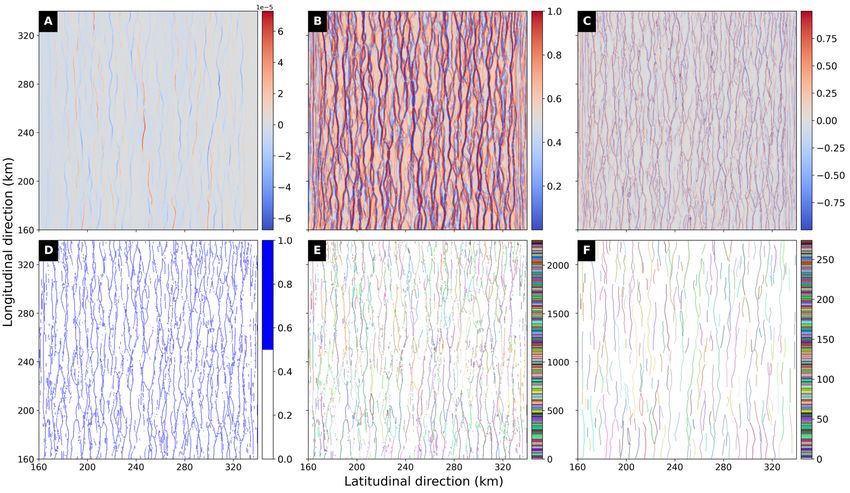
322 Figure 3. End-member behaviour of transient deformation. Along-strike map of a subset of the
323 model that experienced 10 mm yr-1 extension. The strain rate invariant (A), finite strain (B), and
324 extracted faults (C) at 2.1 Myrs reveal localised behaviour. The strain rate (D), finite strain (E)
325 and extracted faults (F) at 2.2 Myrs reveal distributed behaviour.
326
1
327 GSA Data Repository item 2021, containing detailed methods of the forward modelling
328 and fault extraction with reproducible datasets, is available online at
329 www.geosociety.org/pubs/ft20XX.htm, or on request from editing@geosociety.org.Figure 1. The top row shows the strain rate invariant (s-1) in the upper crust (5 km depth), documenting active deformation patterns within the last resolvable time increment (10, 5 and 2.5 Myrs for models ran at 2.5, 5, and 10 mm yr-1 respectively). The bottom row shows their corresponding fault length property extracted from the active deformation field. The spatial extent covers the high-resolution (625 m) portion of the model domain.
Figure 2. Geometric statistics of time-dependent fault properties. A) Fault D-L evolution for the modelled fault network that experienced 5 mm yr-1 extension. D-L geometries of observable faults are plotted in
grey, where different shades correlate to different datasets (references therein). B) The number of active faults throughout model evolution all models. C) The average active length of a given population throughout
model evolution. Note that all three models output 50 timesteps, however the age duration for models deformed at 2.5 mm yr-1, 5 mm yr-1 and 10 mm yr-1 are 10 Myrs, 5 Myrs and 2.5 Myrs respectively.
Figure 3. End-member behaviour of transient deformation. Along-strike map of a subset of the model that experienced 10 mm yr-1 extension. The strain rate invariant (A), finite strain (B), and extracted
faults (C) at 2.1 Myrs reveal localised behaviour. The strain rate (D), finite strain (E) and extracted faults (F) at 2.2 Myrs reveal distributed behaviour.
GSA DATA REPOSITORY Pan, Naliboff, Bell and Jackson
SUPPLEMENTARY MATERIAL
Numerical Simulations
Model Geometry and Resolution
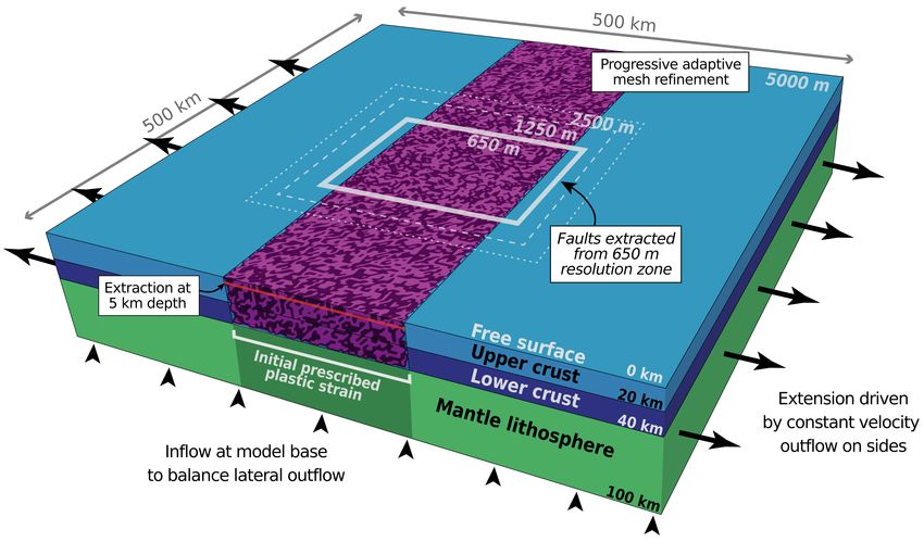
The governing equations are solved on a 3D gridded domain which spans 500 by 500
km across the horizontal plane (X, Y) and 100 km in the depth (Z) direction. The grids are
coarsest (5 km) on the sides and base of the model domain and are successively reduced
using adaptive-mesh refinement, increasing the resolution to 625 m over a centered 180 x 180
x 20 km region (Supplementary Fig. 1). Throughout the model domain we use quadratic
elements (Equation 2) elements to solve the advection-diffusion equation for temperature and
composition, while the Stokes equation is solved on elements that are quadratic for velocity
and continuous linear for pressure (Equations 1 and 2).
Supplemental Figure 1. 3D model setup outlining initial boundary conditions, compositional layers and
prescribed initial strain. Resolution is progressively refined to higher levels up to 650 in the centre, where
we perform fault extraction at 5 km depth.PAN ET AL. SUPPLEMENTARY METHODS
Governing equations
We use the open-source, mantle convection and lithospheric dynamics code ASPECT
(Kronbichler et al., 2012; Heister et al., 2017) to model 3D continental extension following
the approach of Naliboff et al. (2020). The model solves the incompressible Boussinesq
approximation of momentum, mass and energy equations, combined with advection-diffusion
equations which are outlined below. The Stokes equation which solves for velocity and
pressure are defined as:
!⋅# = 0 (1)
−! ⋅ 2 , -̇(#) + !0 = 12 (2)
Where # is the velocity, , is the viscosity, -̇ is the second deviator of the strain rate tensor, 0
is pressure, 1 is density, and 2 is gravitational acceleration.
Temperature evolves through a combination of advection, heat conduction, shear
heating, and adiabatic heating:
56
13! 4 + # ⋅ !68 − ! ⋅ 9:13! ; !6 = 1< + 2= -̇(#) + >6 (# ∙ ∇0) (3)
57
Where 3! is the heat capacity, 6 is temperature, 7 is time, : is thermal diffusivity, and < is
the rate of internal heating. Respectively, the terms on the right-hand side correspond to
internal head production, shear heating, and adiabatic heating.
Density varies linearly as a function of the reference density (1" ), thermal expansivity
(>), reference temperature (6" ) and temperature:
1 = #0 91 − & (' − '0 ); (4)PAN ET AL. SUPPLEMENTARY METHODS
Rheological Formulation
Rheological behaviour combines nonlinear viscous flow with brittle failure (see
Glerum et al., 2018). Viscous flow follows dislocation creep, formulated as:
& & ()* ,
%
B##$ =C ' -̇ '
## D '-. (5)
Above, B##$ is the second invariant of the deviatoric stress, C is the viscous prefactor, F is the
stress exponent, -̇## is the second invariant of the deviatoric strain rate (effective strain rate),
G is the activation energy, H is pressure, I is the activation volume, 6 is temperature, and J
is the gas constant
Brittle plastic deformation follows a Drucker Prager yield criterion, which accounts
for softening of the angle of internal friction (K) and cohesion (3) as a function of
accumulated plastic strain:
6 3 cos K + 2 H sin K
B##$ = (6)
R(3)(3 + sin K)
The initial friction angle and cohesion are 30 and 20 MPa respectively, and linearly weaken
by a factor of 2 as a function of finite plastic strain. We localise deformation in the center of
the model by prescribing an initial plastic strain field. Rather than a single weak seed (e.g.,
Lavier et al., 2000; Thieulot, 2011; Huismans et al., 2007), or randomised distribution (e.g.,
Naliboff et al., 2017; Naliboff et al., 2020; Duclaux et al., 2020), the initial plastic strain field
is partitioned into 5 km coarse blocks which are randomly assigned 0.5 or 1.5. This method
results in statistically random but pervasive damage using an adjustable wavelength (i.e., the
block size) which allows for the adjustment of spatial distribution without changing the
overall initial damage/strain. The data file (composition.txt) containing the initial distribution
of plastic strain and additional compositional field data, as well as the python script to
generate this data (composition.py) are located in the supplementary data set.PAN ET AL. SUPPLEMENTARY METHODS
The viscosity is calculated using the viscosity rescaling method, where if the viscous
stress exceeds plastic yield stress, the viscosity is reduced such that the effective stress
matches the plastic yield (see Glerum et al., 2018). Nonlinearities from the Stokes equations
are addressed by applying defect-Picard iterations (Fraters et al., 2019) to a tolerance of 1e-4.
The maximum numerical time step is limited to 20 kyr.
Initial Conditions
The model domain contains three distinct compositional layers, representing the upper
crust (0-20 km depth), lower crust (20-40 km depth), and lithospheric mantle (40-100 km
depth). Distinct background densities (2700, 2800, 3300 kg m-3) and viscous flow laws for
dislocation creep (wet quartzite (Gleason and Tullis, 1995), wet anorthite (Rybacki et al.,
2003), dry olive (Hirth and Kohlstedt, 2003) distinguish these three layers, which deform
through a combination of nonlinear viscous flow and brittle (plastic) deformation (Glerum et
al., 2018; Naliboff et al., 2020). Supplementary Table 1 contains the specific parameters for
each flow law.
The initial temperature distribution follows a characteristic conductive geotherm for
the continental lithosphere (Chapman, 1986). We solve for the conductive profile by first
assuming a thermal conductivity of 2.5 W m-1 K-1, a surface temperature of 273 K, and a
surface heat flow of 55 mW/m2, and constant radiogenic heating in each compositional layer
(Supplementary Table 1) which we use to calculate the temperature with depth within each
layer. The resulting temperature at the base of the upper crust, lower crust, and mantle
lithosphere, respectively, are 633, 893, and 1613 oK. Supplementary file (geotherm.py)
provides an example of how to calculate the geothermal profile and extract the parameters
required to reproduce this initial profile within the ASPECT parameter file.PAN ET AL. SUPPLEMENTARY METHODS
Supplementary Table 1. Material properties for distinct compositional layers
Compositional layer Upper crust Lower crust Mantle lithosphere
Reference density 2700 kg m-3 2900 kg m-3 3250 kg m-3
Viscosity prefactor (A*) 8.57 x 10⁻²⁸ Pa-n m-p s-1 7.13 x 10⁻¹⁸ Pa-n m-p s-1 6.52 x 10⁻¹⁶ Pa-n m-p s-1
n 4 3 3.5
Activation energy (Q) 223 kJ mol-1 345 kJ mol-1 530 kJ mol-1
Activation volume (V) N/A N/A 18 x 106 m3 mol-1
Specific heat (Cp) 750 J kg-1 k-1 750 J kg-1 k-1 750 J kg-1 k-1
Thermal conductivity (K) 2.5 W m-1 K-1 2.5 W m-1 K-1 2.5 W m-1 K-1
Thermal expansivity (A) 2.5 x 10⁻⁵ K-1 2.5 x 10⁻⁵ K-1 2.5 x 10⁻⁵ K-1
Heat production (H) 1 x 10⁻⁶ W m-3 0.25 x 10⁻⁶ W m-3 0
Friction angle (ϕ) 30 ° 30 ° 30 °
Cohesion angle (C) 20 MPa 20 MPa 20 MPa
Boundary Conditions
Deformation is driven by prescribed outflow velocities on the left and right sides (i.e.,
orthogonal extension), with inflow at the model base exactly balancing the outflow. The top
of the model is a free surface (Rose et al., 2015) and is advected normal to the velocity field.
The extension rate (i.e., the prescribed outward velocity) is 2.5, 5 and 10 mm/yr (Fig. 1).
Compiling and Running ASPECT
The model in this study were run with ASPECT version 2.2.0-pre at commit
ab5eead39. This version of ASPECT can be obtained with git checkout ab5eead39 from the
main branch. The models were run on 720 processors (15 nodes) on Stampede2 (TACC)
through XSEDE allocation TG-EAR180001. Instructions for compiling ASPECT onPAN ET AL. SUPPLEMENTARY METHODS
Stampede2 can be found at https://github.com/geodynamics/aspect/wiki/Compiling-and-
Running-ASPECT-on-TACC-Stampede2.
Fault extraction workflow
Supplemental Figure 2. Workflow for fault extraction, performed at 5 km depth. The outcome of workflow
produces fault labels (F) from which key geometric fault properties can be extracted, such as fault length, strain,
strike and dip.
The input image can be a depth slice of any field documenting strain (e.g., the finite
/0"
plastic strain, strain rate invariant, or components of the velocity vector). Our results use /1
as the input image (A; Supplementary Fig. 2) as this reveals the dip direction of active faults.
The input slice is derived with respect to depth and histogram equalisation is applied (B) in
order to i) allow for areas of lower contrast (i.e., smaller faults) to gain a higher contrast,
enabling a comprehensive extraction of the entire fault population; and ii) globally adjust
contrast for comparison across multiple timesteps. In effect, this step in the workflowPAN ET AL. SUPPLEMENTARY METHODS produces a value of 0 on one side of the fault, and a value of 1 on the other side of the fault (B), such that in the presence of bifurcation, fault segments are separated. The localities of fault segments are revealed by computing the difference between large contrasts along the longitudinal direction (C), and a predetermined fraction of this range is used to threshold the image (D). The binary array is labelled according to neighbouring connectivity (i.e., horizontal, vertical and diagonal) of pixels (E) (Dillencourt et al., 1992). Noise is filtered out by removing labelled pixels which are smaller than 20. In the case that branching remains, a post-processing script breaks up any remaining branches by locating euclidean distance transformation anomalies which arise as a result of bifurcation, and use the locality as a mask to split labels into two discrete fault segments. REFERENCES 1. Chapman, D.S., 1986. Thermal gradients in the continental crust. Geological Society, London, Special Publications, 24(1), pp.63-70. 2. Dillencourt, M.B., Samet, H. and Tamminen, M., 1992. A general approach to connected- component labeling for arbitrary image representations. Journal of the ACM (JACM), 39(2), pp.253-280. 3. Duclaux, G., Huismans, R.S. and May, D.A., 2020. Rotation, narrowing, and preferential reactivation of brittle structures during oblique rifting. Earth and Planetary Science Letters, 531, p.115952. 4. Fraters, M.R., Bangerth, W., Thieulot, C., Glerum, A.C. and Spakman, W., 2019. Efficient and practical Newton solvers for non-linear Stokes systems in geodynamic problems. Geophysical Journal International, 218(2), pp.873-894. 5. Gleason, G.C. and Tullis, J., 1995. A flow law for dislocation creep of quartz aggregates determined with the molten salt cell. Tectonophysics, 247(1-4), pp.1-23. 6. Glerum, A., Thieulot, C., Fraters, M., Blom, C. and Spakman, W., 2018. Nonlinear viscoplasticity in ASPECT: benchmarking and applications to subduction. Solid Earth, 9(2), pp.267-294.
PAN ET AL. SUPPLEMENTARY METHODS

7. Heister, T., Dannberg, J., Gassmöller, R. and Bangerth, W., 2017. High accuracy mantle
   convection simulation through modern numerical methods–II: realistic models and
   problems. Geophysical Journal International, 210(2), pp.833-851.
8. Hirth, G. and Kohlstedf, D., 2003. Rheology of the upper mantle and the mantle wedge:
   A view from the experimentalists. Geophysical Monograph-American Geophysical
   Union, 138, pp.83-106.
9. Huismans, R.S. and Beaumont, C., 2007. Roles of lithospheric strain softening and
   heterogeneity in determining the geometry of rifts and continental margins. Geological
   Society, London, Special Publications, 282(1), pp.111-138.
10. Kronbichler, M., Heister, T. and Bangerth, W., 2012. High accuracy mantle convection
   simulation through modern numerical methods. Geophysical Journal
   International, 191(1), pp.12-29.
11. Lavier, L.L., Buck, W.R. and Poliakov, A.N., 2000. Factors controlling normal fault
   offset in an ideal brittle layer. Journal of Geophysical Research: Solid Earth, 105(B10),
   pp.23431-23442.
12. Naliboff, J.B., Glerum, A., Brune, S., Péron-Pinvidic, G. and Wrona, T., 2020.
   Development of 3-D rift heterogeneity through fault network evolution. Geophysical
   Research Letters, 47(13), p.e2019GL086611.
13. Rose, I., Buffett, B. and Heister, T., 2017. Stability and accuracy of free surface time
   integration in viscous flows. Physics of the Earth and Planetary Interiors, 262, pp.90-
   100.
14. Rybacki, E., Gottschalk, M., Wirth, R. and Dresen, G., 2006. Influence of water fugacity
   and activation volume on the flow properties of fine-grained anorthite aggregates. Journal
   of Geophysical Research: Solid Earth, 111(B3).
15. Thieulot, C., 2011. FANTOM: Two-and three-dimensional numerical modelling of
   creeping flows for the solution of geological problems. Physics of the Earth and
   Planetary Interiors, 188(1-2), pp.47-68.
You can also read