Learning Flexible and Reusable Locomotion Primitives for a Microrobot
←
→
Page content transcription
If your browser does not render page correctly, please read the page content below
IEEE ROBOTICS AND AUTOMATION LETTERS. PREPRINT VERSION. ACCEPTED JANUARY, 2018                                                              1

           Learning Flexible and Reusable Locomotion
                   Primitives for a Microrobot
         Brian Yang, Grant Wang, Roberto Calandra, Daniel Contreras, Sergey Levine, and Kristofer Pister

   Abstract—The design of gaits for robot locomotion can be a
daunting process which requires significant expert knowledge
and engineering. This process is even more challenging for
robots that do not have an accurate physical model, such as
compliant or micro-scale robots. Data-driven gait optimization
provides an automated alternative to analytical gait design. In
this paper, we propose a novel approach to efficiently learn a wide
range of locomotion tasks with walking robots. This approach
formalizes locomotion as a contextual policy search task to collect            Figure 1: The six-legged micro walker considered in our study
data, and subsequently uses that data to learn multi-objective
locomotion primitives that can be used for planning. As a proof-               as a CAD model (left) and an assembled prototype (right).
of-concept we consider a simulated hexapod modeled after a
recently developed microrobot, and we thoroughly evaluate the                  environments designed to simulate dynamics at this scale are
performance of this microrobot on different tasks and gaits. Our               generally unequipped for usage in robotics contexts. Addition-
results validate the proposed controller and learning scheme                   ally, working with microrobots can place severe limitations on
on single and multi-objective locomotion tasks. Moreover, the
experimental simulations show that without any prior knowledge                 the number of iterations as trials become much more time-
about the robot used (e.g., dynamics model), our approach is                   consuming and expensive to run.
capable of learning locomotion primitives within 250 trials and                   While microrobot locomotion has been addressed in the
subsequently using them to successfully navigate through a maze.               past, much of the work is primarily concerned with the
                                                                               mechanical design and manufacturing of microrobots. Ac-
  Index Terms—Learning and Adaptive Systems; Micro/Nano                        complishing more sophisticated locomotion tasks on the sub-
Robots; Legged Robots                                                          centimeter scale remains an open area for research. Analytical
                                                                               implementations of various gait behaviors have worked on
                          I. I NTRODUCTION                                     microrobots [3], [4], but these solutions can become unwieldy
     UBSTANTIAL progress has been made in recent years                         for robots with higher DOF such as legged walkers (e.g., our
S    towards the development of fully autonomous micro-
robots [1], [2]. However, gait design for robot locomotion at
                                                                               micro-hexapod). Data-driven automatic gait optimization is a
                                                                               viable alternative to analytical gait design and optimization,
the sub-centimeter scale is not a well-studied problem. Com-                   but using these techniques can be challenging due to the high
pleting more complicated locomotion tasks like navigating                      number of trials that might be necessary to perform in order
complex environments is even more challenging. These issues                    to learn viable gaits.
become exacerbated when dealing with legged locomotion,                           Our contributions are two-fold: 1) we validate the use of
where even walking straight is still an active area of study for               both CPG controllers and Bayesian optimization for micro-
normal-sized robots. In this paper, we present a novel approach                robots on a wide range of single and multi-objective loco-
for the autonomous optimization of locomotion primitives and                   motion tasks. 2) we introduce a novel approach to efficiently
gaits.                                                                         learn gaits and motor primitives from scratch without the
   While locomotion on larger-scale robots has been thor-                      need for prior knowledge (e.g., a dynamics model). This is
oughly investigated, transferring many of these proven ap-                     accomplished by collecting data on various motor primitives
proaches to the millimeter scale poses many unique challenges.                 using contextual policy search and using those evaluations to
One such obstacle is the lack of access to sufficiently accurate               reformulate the problem into a multi-objective optimization
simulated models at the millimeter scale. Even simulation                      task, providing us a model that can map any set of parameters
                                                                               to a predicted trajectory. Using this model, we can optimize
  Manuscript received: September, 09, 2017; Revised January, 21, 2018;         our parameters on various trajectories for subsequent use
Accepted January, 27, 2018.
  This paper was recommended for publication by Editor Yu Sun upon             in path planning. This approach is not tied exclusively to
evaluation of the Associate Editor and Reviewers’ comments. This work          microrobots, but can be used for any walking robot.
was supported by the Berkeley Sensor and Actuator Center, and by Berkeley         To evaluate our approach, we used a simulated hexapod mi-
DeepDrive. (Brian Yang and Grant Wang contributed equally to this work.)
(Corresponding author: Roberto Calandra)                                       crorobot modeled after the recently developed microrobot [5]
  All the authors are with the Department of Electrical Engineering and Com-   shown in Figure 1. We first validate the use of a CPG
puter Sciences, University of California, Berkeley, USA {brianhyang,           controller on our microrobot to reduce the number of pa-
grant.wang5, roberto.calandra, dscontreras,
ksjp}@berkeley.edu, svlevine@eecs.berkeley.edu                                 rameters during optimization. Then, we validate the use of
  Digital Object Identifier (DOI): 10.1109/LRA.2018.2806083                    Bayesian optimization and existing techniques on a curriculum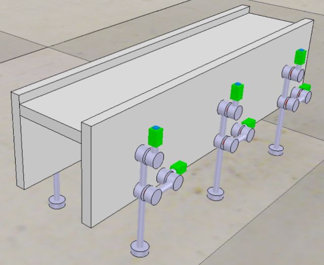
2                                                     IEEE ROBOTICS AND AUTOMATION LETTERS. PREPRINT VERSION. ACCEPTED JANUARY, 2018

of progressively more difficult tasks including learning single-                Motor                 Motor                    Motor
objective, contextual, and multi-objective gaits. As a proof
of concept, we evaluated our approach by learning motor
primitives from 250 trials and subsequently using them to
successfully navigate through a maze.

                                                                        Motor

                                                                                              Motor

                                                                                                                    Motor
                      II. R ELATED W ORK
   There has been an abundance of work published on the
design and development of walking [6] and flying millimeter-
scale microrobots [7], [8], [9]. Much of this work focuses
                                                                      Figure 2: Diagram of the robot leg showing the actuation
on hardware considerations such as the design of micro-sized
                                                                      sequence (active motors are shown in red). Each leg has 2
joints and actuators rather than control. To our knowledge, no
                                                                      motors, each one independently actuating a single DOF.
previous work has implemented a CPG-based controller for
on-board control of a walking microrobot, nor has learning
been used for locomotion on a microrobots.
                                                                      the robot is subject to wear-and-tear, and therefore any learning
   While hexapod gaits have been thoroughly studied and
                                                                      approach employed must be capable of learning gaits within
tested [10], [11], much of the work did not easily transfer to
                                                                      a limited number of trials.
our microrobot due to the drastically different leg dynamics.
Most hexapods make use of rotational joints with higher DOF
while our walker uses only two prismatic spring joints per            A. Physical Description
leg, resulting in less control and unique constraints on leg             The hexapod microrobot is based on silicon microelec-
retraction and actuation.                                             tromechanical systems (MEMS) technology. The robot’s legs
   While sufficient for simple controllers with few parameters,       are made using linear motors actuating planar pin-joint link-
manually tuning controller parameters can require an immense          ages [24]. A tethered single-legged walking robot was previ-
amount of domain expertise and time. As such, automatic               ously demonstrated using this technology [5]. The hexapodal
gait optimization is an important research field that has been        robot is assembled using three chips. The two chips on the side
studied with a wide variety of approaches in both the single-         each have 3 of the leg assemblies, granting six 2 degree-of-
objective [12], [13], [14], [15], [16], [17], [18], [19] and multi-   freedom (DOF) legs for the whole robot. The top chip acts to
objective setting [20], [17], [18], [21]. Evolutionary algorithms     hold the leg chips together for support, and to route the signals
have been successfully used to train quadrupedal robots [13],         for off-board power and control. Overall, the robot measures
[17], but this approach often requires thousands of experiments       13 mm long by 9.6 mm wide and stands at 8 mm tall with an
before producing good results, which is unfeasible on fragile         overall weight of approximately 200 mg.
microrobots.
   A more data-efficient approach used before to learn gaits
                                                                      B. Actuation
for snake and bipedal robots is Bayesian optimization [15],
[16], [19], [22]. Bayesian optimization has been applied to              Each of the robot’s legs has 2-DOF in the plane of fabri-
contextual policy search in the context of robot manipula-            cation, as shown in Figure 2. Both DOFs are actuated, thus
tion [23]. Our contribution builds off of this work by applying       the leg has 2 motors, one to actuate the vertical DOF to
and extending the contextual framework to learning movement           lift the robot’s body and a second to actuate the horizontal
trajectories and path planning. Another extension of Bayesian         DOF for the vertical stride. The actuators used for the legs
optimization related to our work is Multi-objective Bayesian          are electrostatic gap-closing inchworm motors [25]. During a
optimization, which has also been previously applied in the           full cycle, each leg moves 0.6 mm vertically with a horizontal
context of robotic locomotion [21]. However, past work is             stride of 2 mm. For more details on the actuation mechanism
only concerned with using multi-objective optimization to             used on our microrobot, we refer readers to [26].
balance the trade-off between various competing goals. Our
main contribution demonstrates an entirely novel application          C. Simulator
of multi-objective optimization to learning motor primitives
                                                                         In our experimental simu-
that does not involve the trade-off between various goals, but
                                                                      lations, we used the robotics
instead uses a multi-objective model to learn over an area of
                                                                      simulator V-REP [27] for con-
possible trajectories for path planning.
                                                                      structing a scaled-up simulated
                                                                      model of the physical micro-
              III. T HE H EXAPOD M ICROROBOT                          robot (see Figure 3). Since V-
   We now introduce the hexapod microrobot considered in              REP was not designed with
this paper. This robot is of particular interest due to the           simulation of microrobots in
unique challenges that arise when attempting traditional gait         mind, it was not capable of
                                                                                                         Figure 3: The simulated mi-
design techniques. The micro-scale of the walker makes it very        simulating the dynamics of the
                                                                                                         cro walker.
challenging to obtain an accurate dynamics model. Moreover,           leg joints accurately and would
YANG et al.: LEARNING FLEXIBLE AND REUSABLE LOCOMOTION PRIMITIVES FOR A MICROROBOT 3
produce wildly unstable models at the desired scale. We chose and R is the phase difference between each of the vertical-
to scale up the size of the robot in simulation by a factor of 100 horizontal oscillator pairs. In order to allow for directional
in order to account for the issues with scaling in simulation control, Xl and Xr are the amplitudes of the left and right
(all the experimental results are re-normalized to the dimen- side oscillators respectively.
sions of the real robot). We believe that this re-scaling still
allows meaningful results to be produced for several reasons. B. Bayesian Optimization
First, the experiments performed in this paper are meant to
demonstrate the validity of the proposed controller, and the Even with a complete CPG network, some amount of pa-
learning approach for training an actual physical microrobot. rameter tuning is necessary to obtain efficient locomotion. To
The policies trained are not meant to work on the real robot automate the parameter tuning, we use Bayesian optimization
without any re-tuning or modification. Second, the simulator (BO), an approach often used for global optimization of black
still allows to test the basic motion patterns we want to box functions [31], [32], [19]. We formulate the tuning of the
implement on the microrobot. Finally, our contribution lends CPG parameters as the optimization
credibility to the potential application of Bayesian-inspired θ ∗ = arg maxθ f (θ) , (4)
optimization methods to a setting where evaluations can be
costly and time consuming. where θ are the CPG parameters to be optimized w.r.t. the
objective function of choice f (e.g., walking speed, which
IV. BACKGROUND we investigate in Section VI-B). At each iteration, BO learns
a model f˜ : θ → f (θ) from the dataset of the previously
A. Central Pattern Generators
evaluated parameters and corresponding objective values mea-
Central pattern generators (CPGs) are neural circuits found sured D = {θ, f (θ)}. Subsequently, the learned model f˜ is
in nearly all vertebrates, which produce periodic outputs used to perform a “virtual” optimization through the use of
without sensory input [28]. CPGs are also a common choice an acquisition function which controls the trade-off between
for designing gaits for robot locomotion [29]. We chose to use exploration and exploitation. Once the model is optimized,
CPGs for our controller because they are capable of reproduc- the resulting set of parameters θ ∗ is finally evaluated on
ing a wide variety of different gaits simply by manipulating the real system, and is added to the dataset together with
the relative coupling phase biases between oscillators. This the corresponding measurement f (θ ∗ ) before starting a new
allows us to easily produce a variety of gait patterns without iteration. A common model used in BO for learning the
having to manually program those behaviors. In addition, underlying objective, and the one that we consider, is Gaussian
CPGs are not computationally intensive and can have on- processes [33]. For more information regarding BO, we refer
chip hardware implementations using VLSI or FPGA. This the readers to [32], [34].
makes them well suited to be eventually used in our physical
microrobot, where the processing power is limited. CPGs can
C. Multi-objective Bayesian Optimization
be modeled as a network of coupled non-linear oscillators
where the dynamics of the network are determined by the A special case of the optimization task of Equation (4) is
set of differential equations multi-objective optimization [35]. Often times in robotics1 ,
X there are multiple conflicting objectives that need to be op-
φ̇i = ωi + (ωij rj sin(φj − φi − ϕij )) , (1) timized simultaneously, resulting in design trade-offs (e.g.,
j walking speed vs energy efficiency which we investigate
ar in Section VI-C). When multiple objectives are taken into
r¨i = ar ( (Ri − ri ) − r˙i ) , (2)
4 consideration, there is no longer necessarily a single optimum
ax
ẍi = ax ( (Xi − xi ) − ẋi ) , (3) solution, but rather the goal of the optimization became to
4
find the set of Pareto optimal solutions [37], which also
where φi is a state variable corresponding to the phase of the takes the name of Pareto front (PF). Formally, the PF is
oscillations and ωi is the target frequency for the oscillations. the set of parameters that are not dominated, where a set of
ωij and ϕij are the coupling weights and phase biases which parameters θ 1 is said to dominate θ 2 when
change how the oscillators influence each other. To implement
our desired gaits, we only need to modify the phase biases ∀i ∈ {1, . . . , n} : fi (θ 1 ) ≤ fi (θ 2 )
(5)
between the oscillators φij . ri and xi are state variables for ∃j ∈ {1, . . . , n} : fj (θ 1 ) < fj (θ 2 )
the amplitude and offset of each oscillator, and Ri and Xi are Intuitively, if θ 1 θ 2 , then θ 1 is preferable to θ 2 as it
control parameters for the desired amplitude and offset. The never performs worse, but at least in one objective function it
constants ar and ax are constant positive gains and allow us performs strictly better. However, different dominant variables
to control how quickly the amplitude and offset variables can are equivalent in terms of optimality as they represent different
be modulated. A more detailed explanation of the network can trade-offs.
be found in Crespi’s original work [30]. One of the foremost Multi-objective optimization can often be difficult to per-
benefits of using a CPG controller is a drastic reduction in form as it might require a significant amount of experiments.
the number of parameters θ i we need to optimize. Overall, This is especially true with our microrobot where large number
the parameters that we consider during the optimization are
θ = [ω, R, Xl , Xr ] where ω is the frequency of the oscillators 1 As well as in nature [36].4 IEEE ROBOTICS AND AUTOMATION LETTERS. PREPRINT VERSION. ACCEPTED JANUARY, 2018
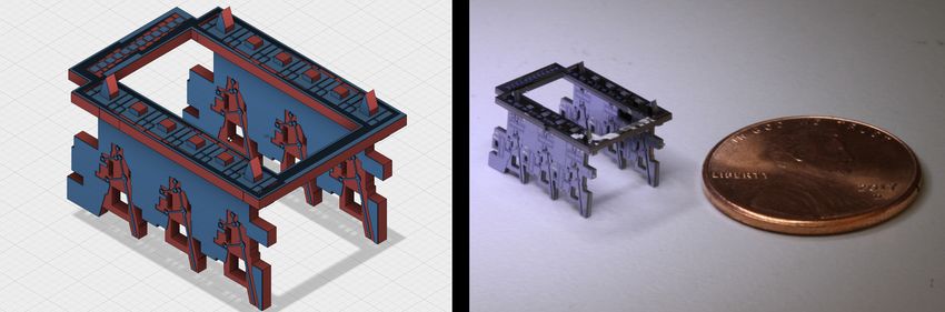
Actuation distance [cm]
of experiments can wear-and-tear the robot. As a result, 0.08 Vertical
Horizontal
the number of evaluations allowed to find the Pareto set of
solutions is limited. Luckily for us, there exist extensions of 0.04
BO which address multi-objective optimization. In particular,
the multi-objective Bayesian optimization algorithm that we 0.00
0.0 0.2 0.4 0.6 0.8
consider is ParEGO [38]. The main intuition of ParEGO is Time [s]
that at every iteration, the multiple objectives can be randomly Figure 4: Output of one vertical-horizontal oscillator pair in
scalarized into a single objective (via the augmented Tcheby- the CPG network, which corresponds to one leg on the robot.
cheff function), which is subsequently optimized as in the stan- The retraction phase of both motors occurs concurrently and
dard Bayesian optimization algorithm (by creating a response rapidly in order to simulate the physical constraints on the
surface, and then optimizing its acquisition function). For more actual physical microrobot.
information about multi-objective Bayesian optimization we
refer the reader to [39]. L1 L1
L2 L2
D. Contextual Bayesian Optimization L3 L3
R1 R1
Another special case of the optimization task of Equa- R2 R2
tion (4), is contextual optimization. In contextual optimization, R3 R3
we assume that there are multiple correlated, but slightly (a) Dual Tripod (b) Ripple
different, tasks which we want to solve, and that they are
L1 L1
identified by a context variable c. An example (which we L2 L2
investigate in Section VI-E) might be walking on inclined L3 L3
slopes, where the contextual variable is the angle of the slope. R1 R1
The contextual optimization can hence be formalized as R2 R2
R3 R3
θ ∗ = arg maxθ f (θ, c) , (6) (c) Wave (d) Four-Two
where for each context c, a potentially different set of param- swing phase retract phase
eters θ ∗ exists. The main advantage compared to treating each Figure 5: Contact/swing patterns for different gaits.
task independently is that, in contextual optimization, we can
exploit the correlation between the tasks to generalize, and as a
f˜ : [θ, ∆xdes , ∆ydes ] → f (θ). However, in order to compute f
result quickly learn how to solve a new context. Specifically,
it would need to measure ∆xobs , ∆yobs , effectively generating
in this paper we consider contextual Bayesian optimization
data of the form
(cBO) [23] which extends the classic BO framework from
Section IV-B. Contextual Bayesian Optimization learns a joint [θ, ∆xdes , ∆ydes ] → [∆xobs , ∆yobs , f (θ)] (8)
model f˜ : {θ, c} → f (θ), but now, at every iteration the ac-
quisition function is optimized with a constrained optimization We can now re-use the data generated from this contextual
where the context c is provided by the environment. However, optimization to learn a motor primitive model in the form
because the model jointly model the context-parameter space, g : θ → [∆xobs , ∆yobs ]. The purpose of this learned model g is
experience learned in one context can be generalized to similar now to provide an estimate of the final displacement obtained
contexts. By utilizing cBO, we will show in Section VI that for a set of parameters independently from the optimization
our microrobot can learn to walk (and generalize) to different process that generated it. Once such a model is learned, we
environmental contexts such as walking uphill and curving. can use it to compute parameters that lead to the desired
displacement ∆x∗obs , ∆yobs
∗
by optimizing the parameters w.r.t.
V. L EARNING L OCOMOTION P RIMITIVES FOR PATH the output of the model
P LANNING
θ ∗ = arg maxθ z(g(θ)) , (9)
We now present our novel approach to learn motor prim-
itives for path planning. This approach relies on the pos- where z is a scalarization function of our choice (e.g., the
sibility of re-using the evaluations collected using cBO to Euclidean distance). This is equivalent to learning a continuous
convert the task into a multi-objective optimization problem. function that generates motor primitives from the desired
We specifically consider a cBO task where we want to displacement. It should be noted that this optimization is
optimize the parameters θ to reach different target positions performed on the model g and therefore does not require any
c = [∆xdes , ∆ydes ] (this setting is evaluated in Section VI-F). physical interaction with the robot. Moreover, we can optimize
The objective function in this case can be defined as the the parameters over a series of multiple displacements to
Euclidean distance obtain a path planning optimization. In Section VI-G, when
q
2 2 performing path planning using the learned motor primitives
f = (∆xdes − ∆xobs ) + (∆ydes − ∆yobs ) , (7)
we will employ a simple shooting method optimization which
where ∆xobs , ∆yobs are the actual positions measured after randomly samples multiple candidate parameters and selects
evaluating a set of parameters. The cBO model would map the best outcome.YANG et al.: LEARNING FLEXIBLE AND REUSABLE LOCOMOTION PRIMITIVES FOR A MICROROBOT 5
1.5 1.5 4 4
Speed [cm/s]
Speed [cm/s]
1.0 1.0 3 3
Power [mW]
Power [mW]
0.5 0.5 2 2
0.0 0.0 1 1
0 20 40 60 80 100 0 20 40 60 80 100
Iteration Iteration
(a) Dual Tripod (b) Ripple 0
0.2 0.0 0.2 0.4 0.6 0.8 1.0
0
0.2 0.0 0.2 0.4 0.6 0.8 1.0
1.5 1.5
Speed [cm/s] Speed [cm/s]
Speed [cm/s]
Speed [cm/s]
1.0 1.0 (a) Dual Tripod (b) Ripple
4 4
0.5 0.5
3 3
Power [mW]
Power [mW]
0.0 0.0
0 20 40 60 80 100 0 20 40 60 80 100
Iteration Iteration 2 2
(c) Wave (d) Four-Two
1 1
Figure 6: Learning curve for the four gaits (median and 65th
0 0
percentile). We can see how, for all the gaits, BO learns to 0.2 0.0 0.2 0.4 0.6 0.8 1.0 0.2 0.0 0.2 0.4 0.6 0.8 1.0
Speed [cm/s] Speed [cm/s]
walk from scratch within 50 iterations. After the optimization,
Dual Tripod and Ripple are the fastest gaits at ∼ 1.1 cm/s and (c) Wave (d) Four-Two
∼ 1.2 cm/s respectively. Figure 7: Performance measured for the four gaits, and the
corresponding PFs. ParEGO is able to quickly explore the PF
for each of our four gaits.
VI. E XPERIMENTAL S IMULATION R ESULTS
In this section, we discuss our controller implementation
as well as the performance of our simulated microrobot difference for the whole network in order to reduce the number
on various locomotion tasks. The code used for perform- of parameters and speed up the rate of convergence. We use
ing the simulation and videos of the various locomotion two separate parameters for amplitude, each controlling the left
tasks are available online at https://sites.google.com/view/ and right set of legs respectively. This choice of parameters
learning-locomotion-primitives. allows us to control the turning of the robot which is necessary
for path planning and corrections for not walking straight.
A. Controller Implementation
We built our controller following the setup described in B. Learning to Walk Straight
Section IV-A, using a network of 12 coupled phase oscillators We optimized the four gaits considered (i.e., dual tripod,
(one per motor). In order to translate the output of each of ripple, wave, and four-two) using as our objective function the
the oscillators into motor actuation, we calculate the oscilla- walking speed of the robot (measured as the distance traveled
tor outputs for each vertical-horizontal motor pair using the after 1 s). Since some gaits result in curved motions, we also
piecewise function penalized the speed objective with a term proportional to the
drift from the axis of locomotion. The optimization used the
xi + ri cos(φi ), xj + rj cos(φj ) if φi > π, φj > π ,
4 parameters outlined in Section IV-A and was repeated 50
x + r , x + r cos(φ )
i i j j j if φi ≤ π, φj > π , times for each of the gaits. In Figure 6, we show the median
(10)
x i + ri , xj + rj if φi ≤ π, φj ≤ π , and 65th percentiles of the best solution obtained so far in the
xi + ri cos(φi ), xj − rj if φi ≤ π, φj > π , trials. The results show that the optimizer was able to learn
to walk from scratch within 50 iterations. Moreover, it can be
where the ith oscillator outputs to its respective vertical motor
noted that the optimized tripod and ripple are the fastest gaits
and the jth oscillator outputs to its respective horizontal motor.
at ∼ 1.1 cm/s and ∼ 1.2 cm/s respectively.
This allows us to discard the parts of the oscillator output that
are not consistent with the physical constraints of the physical
robot, since the actual leg actuators cannot partially retract C. Multi-objective Gait Optimization
(see Figure 4). We choose to mutually couple all six of the In the previous simulation we only considered walking
vertical oscillators (with a coupling weight of 4 to ensure quick speed as our objective. However, for practical gait design,
convergence on stable limit cycles). We refer the reader to [30] energy efficiency is another objective of great interest, partic-
for a more comprehensive discussion of oscillator coupling in ularly when it comes to designing gaits for a microrobot with
CPGs. Each of the horizontal oscillators are also coupled with real energy restrictions. For this reason, we now consider a
their respective vertical oscillator in order to encapsulate the multi-objective optimization setting and compare the different
dynamics of each leg. We chose to implement four different gaits w.r.t. both walking speed, and energy consumption. The
gaits with the CPG – tripod, ripple, wave, and four-two (see energy consumption of the robot was computed by measuring
Figure 5). For a more detailed description of these gaits we the forces exerted by each of the 12 motors along the axis of
refer the reader to [40]. We use the same frequency and phase actuation and calculating the power used to actuate the motors.6 IEEE ROBOTICS AND AUTOMATION LETTERS. PREPRINT VERSION. ACCEPTED JANUARY, 2018
Training Environments
(a) Discovered Gait 1 (b) Discovered Gait 2
swing phase
Speed [cm/s]
retract phase
1.0
9
0.5
8
7 0.0
0 5 10 15 20
6
Incline [degrees]
Power [mW]
5
Figure 10: Performance of the contextual policy (median and
4 65th percentile) for a wide range of inclines. The policy was
trained only at 5, 10 and 15 degrees, but it was capable of
3
generalizing smoothly to unseen inclinations.
2
PF Unconstrained
1
PF Combined Gait D. Discovering New Gaits with Multi-objective Optimization
0
0.2 0.0 0.2 0.4 0.6 0.8 1.0 1.2 1.4 In addition to optimizing the four nature-inspired gaits,
Speed [cm/s] we also tested multi-objective optimization on the walker
without constraining to using predefined gaits. To parametrize
Figure 9: PF of the unrestrained gait optimization versus the
the oscillator couplings, we thus discretized each gait into
best performance of the four nature-inspired gaits. The faster
intervals of constant length. Within each of these intervals, we
solutions outperform the fastest nature-inspired gaits, albeit
assume that each leg steps exactly once, keeping each of the
with more energy expenditure. However, the inability of the
oscillators in the CPG in phase with each other. This allows us
optimizer to match the performance of the gaits at lower
to parametrize gaits by assigning each leg a point during each
speeds within 1250 trials shows that the gait parametrization
interval where it begins stepping. While this parametrization
can help limit the search space to find better solutions easier.
excludes certain gaits that cannot be expressed in this form,
(top) Pattern for two of the discovered gaits.
we leave the study of more sophisticated gait parameterizations
for gait discovery to future works.
The resulting multi-objective optimization task had 8 pa-
Since the retraction of the legs is spring powered, the energy rameters (frequency, phase difference between horizontal and
input in the cycle is only during motor extension. Hence, we vertical motors, and the six gait coupling parameters). Due to
only consider the cost of extending the legs. With the mass of the higher parameter dimensionality, and because this training
the robot and the time of each trial being held constant, we was not intended for on-line training, we ran the optimization
quantify the energy efficiency of a gait and estimate the cost for 250 iterations in order to allow a more comprehensive
of transport. exploration of the optimization space. We also repeated the
optimization five times for a total of 1250 trials. In Figure 9
We optimized the four 3.5
Dual Tripod
we can see the Pareto front for the resulting gaits. We
gaits again with the same 4 3.0
Ripple
Wave found that the fastest discovered gaits were actually able to
parameters as the previous Four-Two
2.5 outperform the four nature-inspired gaits implemented by a
optimization, but this
Power [mW]
2.0 substantial margin. Even while penalizing curved paths, the
time using multi-objective
fastest discovered gait outperformed Ripple (the fastest nature-
Bayesian optimization 1.5
inspired gait we found) by almost 50%. However, for low-
with a budget of 50 1.0
speed gaits, the nature inspired gaits out-perform the gaits
iterations. In Figure 7 we 0.5
produced by the unconstrained optimization, indicating the
can see the performance 0.0 optimization did not yet fully converged to the optimal PF.
measured and Pareto 0.0 0.2 0.4 0.6 0.8
Speed [cm/s]
fronts obtained for the
different gaits. To better Figure 8: Comparison of the PFs E. Learning to Walk on Inclined Surfaces
compare the PF from the obtained for the different gaits. We now consider the case of contextual optimization and
different gaits, we also specifically the task of gait optimization for slopes with
visualized just the PFs together in Figure 8. From these different inclinations. We framed learning to walk on inclined
results, we can see how the tripod gait dominates the other terrain as a contextual policy search, where the angle of the
gaits for speed < 0.6 cm/s, while Ripple dominates when the inclination is the context. In this simulation, we decided to
speed is > 0.6 cm/s, hence giving a clear indication of which use Dual Tripod for our gait with mostly the same open
gait is preferable under different circumstances. parameters as the previous simulations. We used a singleYANG et al.: LEARNING FLEXIBLE AND REUSABLE LOCOMOTION PRIMITIVES FOR A MICROROBOT 7
6 6 4
Target y-displacement [cm]
Distance to target [cm]
Target y-displacement [cm]
Distance to Target [cm]
1.0
3 Contextual 5 5
Speed [cm/s]
Normal 4 4 3
2
0.5
3 3
Contextual 2 2
2
1
Normal 1 1
1
0.0 0 0 0
0 5 10 15 20 25 30 35 0 10 20 30 40 50
Iteration Iteration 6 4 2 0 2 4 6 6 4 2 0 2 4 6
Target x-displacement [cm] Target x-displacement [cm] 0
(a) Inclined surface. (b) Curved trajectory. (a) cBO (b) Our approach
Figure 11: Comparison between the optimization performance Figure 12: Comparison of the performances of cBO and
of a contextual optimizer and a normal optimizer for two our approach for learning motor primitives (using the same
different tasks: (a) walking on inclines (b) walking curved data). With the robot having an initial position of (0, 0), we
trajectories. In both cases, the contextual optimizer can lever- evaluated the error between the desired position (indicated by
age prior simulations to obtain high-performing gaits in fewer the element of the grid) and the reached position. Darker color
simulations. indicates better target accuracy. While cBO accurately learned
trajectories near the training targets, it did not generalize
parameter to represent the amplitude for the entire network in well to unseen targets. In contrast, our approach had a more
order to keep the number of parameters low with the addition comprehensive coverage as it could leverage better information
of a contextual variable, leaving us with 3 parameters and 1 about the environment to improve generalization.
contextual parameter. To respect real world constraints, where
testing randomly sampled incline angles over a continuous
interval can be excessively time-consuming, we chose at G. Learning Motor Primitives for Path Planning
training time to perform simulations only from a small number In the previous simula-
of inclines: 5, 10, and 15 degrees. tion we learned motor prim- End
After optimizing the gaits for these three inclines over itives capable of walking
50 iterations, we studied how the contextual optimizer is curved trajectories. While
able to generalize across the context space by testing the the model handled trajec-
performance of the contextual policy for a wide range of tories near and between
inclines. In Figure 10 we can see that the policy performs well the targets quite well, the
on intermediary inclines and seems to smoothly interpolate performance on trajectories
between the training inclines as is desirable. The gradual well within the physical ca-
decrease in performance as the inclines get steeper can be pabilities of the robot but
Start
attributed to the increasing physical difficulty for climbing not in proximity to the tar-
up steeper inclines. We also compared cBO against using gets left much to be desired, Figure 13: Path constructed us-
standard BO to train the robot for an untested incline. As as shown in Figure 12. We ing the locomotion primitives
shown in Figure 11a, the contextual optimization was able now demonstrate how our learned with our approach.
to converge on optimal performance significantly faster than approach presented in Sec-
standard BO. This result demonstrate the ability of cBO tion V can be used to significantly improve the movement
to efficiently use data accumulated in previous contexts to accuracy (compared to cBO using the same data), as well as
quickly reach optimize gaits in new unseen contexts. how such motor primitives can be used to perform path plan-
ning. First, we reused the data from the previous simulation in
F. Learning to Curve order to reformulate the task as a multi-objective optimization
Another useful task that can be framed as contextual opti- as described in Section V. Then, we used our trained model
mization is learning motor primitives to walk curved trajecto- to sample 10,000 trajectories by randomly sampling from the
ries for use in path planning. We used the same parameters parameter space. Out of all these trajectories, we selected the
as in Section VI-B and the contextual parameters in this case one with the smallest expected error subject to not walking
were the target displacements along both the x and y axes from through the wall. Evaluating the resulting sequence of motor
the point of origin. In order to train particular trajectories, primitives on the real system (i.e., the simulator) demonstrated
we selected five evenly spaced target points along the front that the expected trajectory was capable of navigating the
quadrant of the field of vision. Since the primary objective maze, as shown in Figure 13.
was to reach the desired destination, we chose to use the
distance of the final position to the target position as our VII. C ONCLUSION
sole objective function. We found that over 10 repetitions, the Designing controllers for locomotion is a daunting task. In
walker was able to accurately move and turn towards all of the this paper, we demonstrated on a simulated microrobot that
target points within 250 iterations. In Figure 11b, we compared this process can be significantly automated. Our main contri-
the performance of cBO against standard BO on a previously butions are two-fold: 1) we introduced a coherent curriculum
unseen target position (4 cos π/16, 4 sin π/16). We found that, of increasing challenging tasks, which we use to evaluate the
as in the case of inclinations, the contextual policy was able CPG controller of our microrobot using Bayesian optimization.
to learn the optimal parameters for a novel trajectory within 2) we presented a new approach that enables walking robots
very few iterations. to efficiently learn motor primitives from scratch. By using the8 IEEE ROBOTICS AND AUTOMATION LETTERS. PREPRINT VERSION. ACCEPTED JANUARY, 2018
data collected from contextual optimization we reformulate the
[16] M. Tesch, J. Schneider, and H. Choset, “Using response surfaces and
problem into a multi-objective optimization task, and learn a expected improvement to optimize snake robot gait parameters,” in
model that can map any set of parameters to a predicted trajec- International Conference on Intelligent Robots and Systems (IROS).
tory. This model can subsequently be used for path planning. IEEE, 2011, pp. 1069–1074.
[17] M. Oliveira, L. Costa, A. Rocha, C. Santos, and M. Ferreira, “Multi-
Our experimental simulation results demonstrate that using objective optimization of a quadruped robot locomotion using a genetic
this approach a microrobot can successfully learn accurate algorithm,” in Soft Computing in Industrial Applications. Springer,
locomotion primitives within 250 trials, and subsequently use 2011, vol. 96, pp. 427–436.
[18] M. Oliveira, V. Matos, C. P. Santos, and L. Costa, “Multi-objective
them to navigate through a maze, without any prior knowledge parameter CPG optimization for gait generation of a biped robot,” in
about the environment or its own dynamics. IEEE International Conference on Robotics and Automation (ICRA),
The gaits obtained on the simulated microrobot might 2013, pp. 3130–3135.
[19] R. Calandra, A. Seyfarth, J. Peters, and M. P. Deisenroth, “Bayesian op-
not yield good results when applied to the real microrobot, timization for learning gaits under uncertainty,” Annals of Mathematics
due to the low-fidelity of the simulator used. However, the and Artificial Intelligence (AMAI), vol. 76, no. 1, pp. 5––23, 2015.
methodology used to obtain them is realistically applicable [20] G. Capi, M. Yokota, and K. Mitobe, “A new humanoid robot gait genera-
tion based on multiobjective optimization,” in IEEE/ASME International
to real microrobots, and is uniquely able to address concerns Conference on Advanced Intelligent Mechatronics, 2005, pp. 450–454.
that exist on the sub-centimeter scale (e.g., lack of a precise [21] M. Tesch, J. Schneider, and H. Choset, “Expensive multiobjective
physics simulator and budgeting of physical experiments). In optimization for robotics,” in International Conference on Robotics and
Automation (ICRA), 2013, pp. 973 – 980.
future work, we plan to evaluate our approach and findings on [22] R. Antonova, A. Rai, and C. G. Atkeson, “Deep kernels for optimizing
the physical hexapod microrobot. locomotion controllers,” in Conference on Robot Learning (CoRL), 2017,
pp. 47–56.
[23] J. H. Metzen, A. Fabisch, and J. Hansen, “Bayesian optimization for
R EFERENCES contextual policy search,” in IROS Workshop on Machine Learning in
[1] K. Saito, K. Iwata, Y. Ishihara, K. Sugita, M. Takato, and F. Uchikoba, Planning and Control of Robot Motion, 2015.
“Miniaturized Rotary Actuators Using Shape Memory Alloy for Insect- [24] D. S. Contreras and K. S. J. Pister, “Durability of silicon pin-joints for
Type MEMS Microrobot,” Micromachines, vol. 7, no. 4, 2016. microrobotics,” International Conference on Manipulation, Automation
[2] D. Vogtmann, R. S. Pierre, and S. Bergbreiter, “A 25 mg magnetically and Robotics at Small Scales (MARSS), pp. 1–6, 2016.
actuated microrobot walking at > 5 body lengths/sec,” in IEEE Interna- [25] I. Penskiy and S. Bergbreiter, “Optimized electrostatic inchworm motors
tional Conference on Micro Electro Mechanical Systems (MEMS), Jan using a flexible driving arm,” Journal of Micromechanics and Microengi-
2017, pp. 179–182. neering, vol. 23, no. 1, Jan. 2013.
[3] T. Ebefors, J. U. Mattsson, E. Kälvesten, and G. Stemme, “A walking [26] D. S. Contreras and K. S. J. Pister, “Dynamics of electrostatic inchworm
silicon micro-robot,” in Proc. Transducers’ 99, 1999, pp. 1202–1205. motors for silicon microrobots,” International Conference on Manipula-
[4] S. Hollar, A. Flynn, C. Bellew, and K. S. J. Pister, “Solar powered 10 tion, Automation and Robotics at Small Scales (MARSS), pp. 1–6, 2017.
mg silicon robot,” in IEEE International Conference on Micro Electro [27] “Robot simulator V-REP,” http://www.coppeliarobotics.com/, 2018.
Mechanical Systems (MEMS). IEEE, 2003, pp. 706–711. [28] J. Yu, M. Tan, J. Chen, and J. Zhang, “A survey on CPG-inspired
[5] D. S. Contreras, D. S. Drew, and K. S. Pister, “First steps of a millimeter- control models and system implementation,” IEEE Transactions on
scale walking silicon robot,” in International Conference on Solid-State Neural Networks and Learning Systems, vol. 25, pp. 441–456, 2014.
Sensors, Actuators and Microsystems (TRANSDUCERS). IEEE, 2017, [29] A. J. Ijspeert, “Central pattern generators for locomotion control in
pp. 910–913. animals and robots: a review,” Neural networks, vol. 21, no. 4, pp. 642–
[6] F. D. Ambroggi, L. Fortuna, and G. Muscato, “PLIF: piezo light 653, 2008.
intelligent flea-new micro-robots controlled by self-learning techniques,” [30] A. Crespi, D. Lachat, A. Pasquier, and A. J. Ijspeert, “Controlling
in International Conference on Robotics and Automation (ICRA), vol. 2, swimming and crawling in a fish robot using a central pattern generator,”
Apr 1997, pp. 1767–1772. Autonomous Robots, vol. 25, no. 1-2, pp. 3–13, dec 2007.
[7] R. J. Wood, “The first takeoff of a biologically inspired at-scale robotic [31] H. J. Kushner, “A new method of locating the maximum point of an
insect,” IEEE Transactions on Robotics, vol. 24, pp. 341–347, 2008. arbitrary multipeak curve in the presence of noise,” Journal of Basic
[8] D. S. Drew and K. S. J. Pister, “First takeoff of a flying microrobot Engineering, vol. 86, pp. 97–106, 1964.
with no moving parts,” in International Conference on Manipulation, [32] D. R. Jones, “A taxonomy of global optimization methods based on
Automation and Robotics at Small Scales (MARSS), 2017, pp. 1–5. response surfaces,” Journal of Global Optimization, vol. 21, no. 4, pp.
[9] B. G. Kilberg, D. S. Contreras, J. Greenspun, and K. S. J. Pister, “Mems 345–383, 2001.
aerodynamic control surfaces for millimeter-scale rockets,” International [33] C. E. Rasmussen and C. K. I. Williams, Gaussian Processes for Machine
Conference on Manipulation, Automation and Robotics at Small Scales Learning. The MIT Press, 2006.
(MARSS), pp. 1–5, 2017. [34] B. Shahriari, K. Swersky, Z. Wang, R. P. Adams, and N. de Freitas,
[10] R. Altendorfer, N. Moore, H. Komsuoglu, M. Buehler, H. Brown, “Taking the human out of the loop: A review of Bayesian optimization,”
D. McMordie, U. Saranli, R. Full, and D. E. Koditschek, “Rhex: A Proceedings of the IEEE, vol. 104, no. 1, pp. 148–175, 2016.
biologically inspired hexapod runner,” Autonomous Robots, vol. 11, [35] J. Branke, K. Deb, K. Miettinen, and R. Slowiński, Multiobjective
no. 3, pp. 207–213, 2001. optimization: interactive and evolutionary approaches. Springer, 2008,
[11] A. M. Hoover, E. Steltz, and R. S. Fearing, “Roach: An autonomous vol. 5252.
2.4 g crawling hexapod robot,” in IEEE/RSJ International Conference [36] D. F. Hoyt and C. R. Taylor, “Gait and the energetics of locomotion in
on Intelligent Robots and Systems (IROS). IEEE, 2008, pp. 26–33. horses,” Nature, vol. 292, no. 5820, pp. 239–240, 1981.
[12] R. Tedrake, T. W. Zhang, and H. S. Seung, “Stochastic policy gradient [37] V. Pareto, Manuale di Economia Politica, 1906, vol. 13.
reinforcement learning on a simple 3d biped,” in IEEE/RSJ International [38] J. Knowles, “ParEGO: A hybrid algorithm with on-line landscape ap-
Conference on Intelligent Robots and Systems (IROS), vol. 3. IEEE, proximation for expensive multiobjective optimization problems,” IEEE
2004, pp. 2849–2854. Transactions on Evolutionary Computation, vol. 10, no. 1, pp. 50–66,
[13] S. Chernova and M. Veloso, “An evolutionary approach to gait learn- January 2006.
ing for four-legged robots,” in International Conference on Intelligent [39] T. Wagner, M. Emmerich, A. Deutz, and W. Ponweiser, “On expected-
Robots and Systems (IROS), vol. 3. IEEE, 2004, pp. 2562–2567. improvement criteria for model-based multi-objective optimization,” in
[14] C. Niehaus, T. Röfer, and T. Laue, “Gait optimization on a humanoid Parallel Problem Solving from Nature (PPSN) XI, 2010, pp. 718–727.
robot using particle swarm optimization,” in Proceedings of the Second [40] R. Campos, V. Matos, and C. Santos, “Hexapod locomotion: A nonlinear
Workshop on Humanoid Soccer Robots, 2007. dynamical systems approach,” in Annual Conference of IEEE Industrial
[15] D. J. Lizotte, T. Wang, M. Bowling, and D. Schuurmans, “Automatic Electronics Society (IECON), Nov 2010, pp. 1546–1551.
gait optimization with Gaussian process regression,” in International
Joint Conference on Artificial Intelligence (IJCAI), 2007, pp. 944–949.You can also read