RICE GRAIN DISEASE IDENTIFICATION USING DUAL PHASE CONVOLUTIONAL NEURAL NETWORK BASED SYSTEM AIMED AT SMALL DATASET
←
→
Page content transcription
If your browser does not render page correctly, please read the page content below
R ICE GRAIN DISEASE IDENTIFICATION USING DUAL PHASE
                                        CONVOLUTIONAL NEURAL NETWORK BASED SYSTEM AIMED AT
                                                          SMALL DATASET

                                                                                                A P REPRINT
arXiv:2004.09870v2 [cs.CV] 7 May 2021

                                                      Tashin Ahmed∗              Chowdhury Rafeed Rahman                    Md. Faysal Mahmud Abid

                                                                                                May 11, 2021

                                                                                               A BSTRACT
                                                    Although Convolutional neural networks (CNNs) are widely used for plant disease detection, they
                                                    require a large number of training samples while dealing with wide variety of heterogeneous back-
                                                    ground. In this paper, a CNN based dual phase method has been proposed which can work effectively
                                                    on small rice grain disease dataset with heterogeneity. At the first phase, Faster RCNN method is
                                                    applied for cropping out the significant portion (rice grain) from an image. This initial phase results
                                                    in a secondary dataset of rice grains devoid of heterogeneous background. Disease classification
                                                    is performed on such derived and simplified samples using CNN architecture. Comparison of the
                                                    dual phase approach with straight forward application of CNN on the small grain dataset shows the
                                                    effectiveness of the proposed method which provides a 5 fold cross validation accuracy of 88.92%.

                                        Keywords Faster RCNN · Dual phase detection · Small dataset · Rice grain · Convolution

                                        1       Introduction
                                        As rice grain diseases occur at the very last moment ahead of harvesting, it does major damage to the cultivation process.
                                        The average loss of rice due to grain discolouration [1] was 18.9% in India. Yield losses caused by False Smut (FS) [2]
                                        ranged from 1.01% to 10.91% in Egypt. 75% yield loss of grain occurred in India in 1950, while in the Philippines [3]
                                        more than 50% yield loss was recorded. Rice yield loss is a direct consequence of Neck Blast (NB) disease, since this
                                        disease results in poor panicles. A big reason behind Neck Blast [4] is an extreme phase of the Blast and grain disease.
                                        In Bangladesh False Smut was one of the most destructive rice grain disease [5] from year 2000 to 2017.
                                        Collecting field level data on agronomy is a challenging task in the context of poor and developing countries. The
                                        challenges include lack of equipment and specialists. Farmers of such areas are ignorant of technology use which makes
                                        it quite difficult to collect crop disease related data efficiently using smart devices via the farmers. Hence, scarcity of
                                        plant disease oriented data is a common challenge while automating disease detection in such areas.
                                        Many researches have been undertaken with a view to automating plant disease detection utilizing different techniques
                                        of machine learning and image processing. [6] through system with the ability to identify areas which contain
                                        abnormalities. They applied a threshold based clustering algorithm for this task. A framework have been created [7] for
                                        the detection of defected diseased leaf using K-Means clustering based segmentation. They claimed that their approach
                                        was able to detect the healthy leaf area and defected diseased area accurately. A genetic algorithm has been developed
                                        [8] which was used for selecting essential traits and optimal model parameters for the SVM classifiers for Bakanae
                                        gibberella fujikuroi disease. A technique to classify the diseases based on percentage of RGB value of the affected
                                        portion was proposed [9] utilizing image processing. A similar technique using multi-level colour image thresholding
                                        was proposed [10] for RLB disease detection. Deep learning based object classification and segmentation has become
                                        the state-of-the-art for automatic plant disease detection. Neural network was employed [11] for leaf disease recognition
                                        while a self organizing map neural network (SOM-NN) was used [12] to classify rice disease images. Researchers also
                                            ∗
                                                corresponding author: tashinahmed@aol.com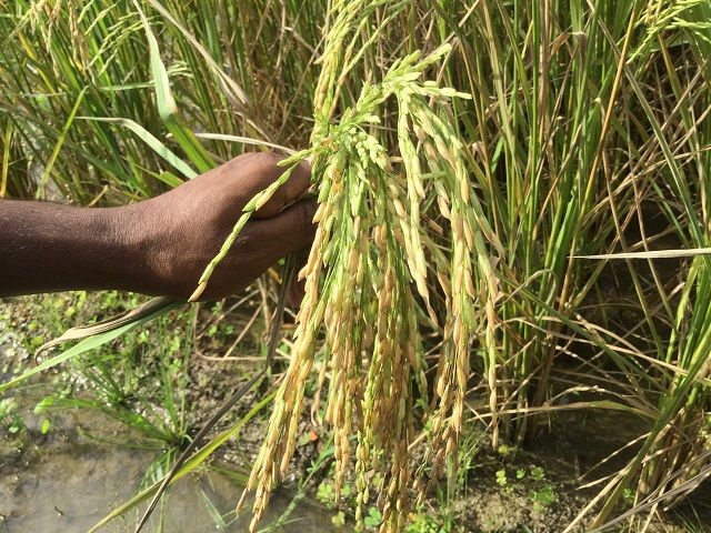
A PREPRINT - M AY 11, 2021
(a) (b) (c)
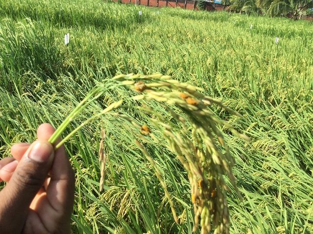
Figure 1: Sample image of every grain classes. From left: (a) False Smut, (b) Healthy and (c) Neck Blast. Images
clearly show the complexity of the dataset where foreground and background are quite identical.
Image Image
Class
Count Percentage
False Smut 75 37.5
Neck Blast 63 31.5
Healthy 62 31.0
Table 1: Image count and percentage(%) of each class of the primary dataset.
experimented with AlexNet [13] to distinguish among 3 classes of rice disease using a small dataset containing 227
images. A similar research for classifying 10 classes of rice disease on a 500 image dataset was undertaken [14] using a
handmade deep CNN architecture. Furthermore, the benefit of using pre-trained model of AlexNet and GoogleNet [15]
has been demonstrated when the training data is not large. Their dataset consisted of 9 diseases of tomatoes. A detailed
comparative analysis of different state-of-the-art CNN baseline and finely tuned architecture [16] on eight classes of
rice disease and pest also conveys a huge potential. It demonstrates two-stage training approach for memory efficient
small CNN architectures. Besides works on rice disease some experimental procedure on other agricultural elements
are, [17] specialized deep learning models based on specific CNN architectures for identification of plant leaf diseases
with a dataset containing 58 classes from 25 different plants have been developed. Transfer learning approach using
GoogleNet [18] on a dataset containing 87848 images of 56 diseases infecting 12 plants. Extraction of disease region
from leaf image through different segmentation [19] techniques was a driving step. Some of the image segmentation
algorithms were compared [20] in order to segment the diseased portion of rice leaves.
Though the above mentioned researches have a significant contribution to the automation of disease detection, none of
the works addressed the problem of scarcity of data which limits the performance of CNN based architectures. Most
of the researches focused on image augmentation techniques to tackle the dataset size issue. But applying different
geometric augmentations on small size images [21, 22] result in nearly the same type of image production which has
drawbacks in terms of neural network training. Production of similar images through augmentation [23] can cause
overfitting as well.
The first phase of the proposed method deals with a learning oriented segmentation based architecture. This architecture
helps in detecting the significant grain portion of a given image that has a heterogeneous background, which is an easier
task compared to disease localization. The detected grain portions cropped from the original image are used as separate
simplified images. In the second phase, these simplistic grain images are used in order to detect grain disease using
fine tuned CNN architecture. Because of the simplicity of the tasks assigned in the two phases, our proposed method
performs well in spite of having only 200 images of three classes. To prove the proposed approach is satisfactory for a
small dataset, counter experimentations on straightforward CNN and Faster RCNN were also demonstrated at Section 4.
2 Our Dataset
Our balanced dataset of 200 images consists of three classes - False Smut, Neck Blast and healthy grain class as shown
in Table 1.
A sample image from each class has been shown in Figure. 1. Neck Blast is generally caused by the fungus known as
Magnaporthe oryzae. It causes plants to develop very few or no grains at all. Infected nodes result [24] in panicle break
2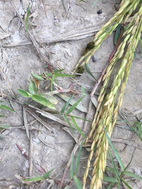
A PREPRINT - M AY 11, 2021

                 (a)                                       (b)                                       (c)

                 (d)                                       (e)                                       (f)

                 (g)                                      (h)                                         (i)
Figure 2: Sample of data heterogeneity amongst the dataset which demonstrates different parameters like unique
backgrounds, lights, contrast, distance have been taken into account while data was gathered. Red rectangular boxes
show how the annotation process has been performed. (a, d, f): multiclass images consists of Neck Blast and False
Smut, (b): healthy, (c, e, h): False Smut, (g, i): Neck Blast.

down. False Smut is caused by the fungus called Ustilaginoidea virens. It results in lower grain weight and reduction
[25] of seed germination.
Data have been collected and annotated from two separate sources for this experiment - field data supervised by officials
from Bangladesh Rice Research Institute (BRRI) and image data from a previously expermineted [16] repository.
As Boro species have the maximum threat to be affected with False Smut and Neck Blast, Boro rice plant has been
chosen [26] for experimental data collection. Parameters like light, distance and uniqueness have been taken into
consideration while capturing the photographs. The main parameter which was taken into account was heterogeneity of
the background. Some sample images of hetergenous background of the dataset have been presented in Figure. 2.
To make the dataset more challenging multiclass images also have been taken into account. Sample images of multiclass
data which consists both Neck Blast and False Smut class have been presented in Figure. 3. If there is a multiclass data
it had been labelled as Neck Blast for the training phase of counter experiments (explained in Section 4) as False Smut
already surpassed by quantity than Neck Blast. Also, the dataset was split into 80:20 in terms of train and validation
set. Augmentation techniques were not applied as the main goal of this experiment is to use small and natural scene
image data. Additionally, there are other factors that can spoil the experiment, such as illumination, symptom severity,
maturity of the plant and diseases. A large versatile dataset can attend on that occasion which can be achieved in the
future. The dataset has been kept to three classes for the early stages of the investigation. Also, it is quite challenging

                                                            3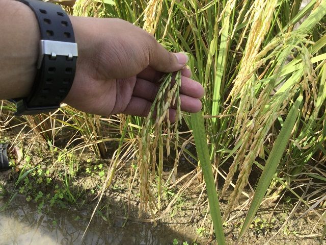
A PREPRINT - M AY 11, 2021

              Figure 3: Sample multiclass data; Labeled green for Neck Blast and red for False Smut class

and burdensome to collect different rice disease image dataset throughout the year as different diseases occur at different
time. So, at this early stage of the investigation three classes is competent to deliver a sufficient result. Supplementary
public data related to the paper can be found at https://cutt.ly/RvgxoDi.

3     Materials and Methods
3.1     Experimental Setup

This subsection explained about the experimental setup which includes hardware used in this experiment and explains
five basenets applied. This subsection have also discussed about different hyperparameter optimization and their
consequence in this experiment.

3.1.1    Hardware
For the training environment, assistance has been taken from two different sources.

         • Royal Melbourne Institute of Technology (RMIT) provides GPU for international research enthusiasts and
           they provided a Red Hat Enterprise Linux Server along with the processor Intel Xeon E5-2690 CPU, clock
           speed of 2.60 GHz. It has 56 CPUs with two threads per core, 503 GB of RAM. Each user can use up to 1
           petabyte of storage. There are also two 16 GB NVIDIA Tesla P100-PCIE GPUs available. First phase was
           completed through this server.
         • Google Colab (Tesla K80 GPU, 12GB RAM) and Kaggle kernel (Tesla P100 GPU) have been used for counter
           experimentation.

3.1.2    Utilized CNN Models
Experiments have been performed using five state-of-the-art CNN architectures which are described as follows. Figure.
4 shows architectures and key blocks of the applied CNN architectures.

VGG16 is a sequential architecture [27] consisting of 16 convolutional layers. Kernel size in all convolution layers is
      three.
VGG19 has three extra convolutional layers [27] and the rest is the same as VGG16.
ResNet50 belongs to the family of residual neural networks. It is a deep CNN architecture [28] with skip connections
       and batch normalization. The skip connections help in eliminating the gradient vanishing problem.
InceptionV3 is a CNN architecture [29] with parallel convolution branching. Some of the branches have filter size as
        large as 7 × 7.
Xception takes the principles of Inception to an extreme. Instead of partitioning the input data into several chunks, it
        maps the spatial correlations [30] for each output channel separately and performs 1 × 1 depthwise convolution.

                                                            4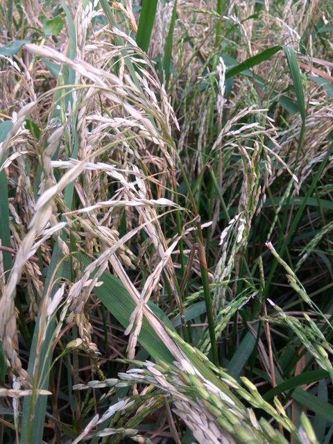
A PREPRINT - M AY 11, 2021

  INPUT               INPUT                  Xl                  Previous                                                     Output
                                                                  Layer                                                      Channels
 Conv - 1            Conv - 1
                                                                                                                                        3X3
 Conv - 2      X2    Conv - 2    X2                                         1X1     3X3
                                                        weight
  Pooling             Pooling                                               Conv    Conv                                                3X3
                                                         BN
 Conv - 1            Conv - 1                                               1X1     5X5        Filter                                   3X3
                                                                            Conv    Conv   Concatenation

                                                                                                              INPUT
 Conv - 2            Conv - 2                           ReLU                                                          1X1
               X3                                                                                                                       3X3   Concat
 Conv - 3            Conv - 3    X3                                                                                   Conv
                                                        weight           3X3        1X1
  Pooling            Conv - 4                                            Max                                                            3X3
                                                                                    Conv
                      Pooling                            BN             Pooling
  Dense                                                                                                                                 3X3
  Dense               Dense               addition                          1X1
                                                                                                                                        3X3
  Dense               Dense                                                 Conv
                      Dense                ReLU
 OUTPUT
                     OUTPUT                Xl+1

    (a)                   (b)                     (c)                              (d)                                             (e)
Figure 4: (a): all 16 blocks of VGG16, (b): all 19 blocks of VGG19, (c): Resdiual module of ResNet, (d): Inception
module is to act as a multi-level feature extractor in InceptionV3, (e): Extreme module of the Inception module which
is utlized in Xception.

                    Hyperparameter            Optimized Value
                    Anchor Box Count          9, 16
                    Anchor Box Size (pixels) [32, 64, 128, 256], [128, 256, 512]
                    Anchor Box Ratios         [(1,1), (2,1), (1,2)], [(1,1), ( √12 , √22 ), ( √22 , √12 ), (2,2)]
                    RPN Threshold             0.3 - 0.7, 0.4 - 0.8
                    Proposal Selection        200, 2000
                    Overlap Threshold         >0.8, >0.9
                    Learning Rate             0.001, 0.0001, 0.00001
                    Optimizers                Adam, SGD
               Table 2: Experimented hyperparameters. Bold values were selcted for the prime experiment.

3.1.3       Optimized Hyperparameters
Hyperparameters of Faster RCNN have been presented in Table 2.

Anchor Box Hyperparameters: Anchor boxes are a set of bounding boxes defined through different scales and aspect
       ratios. They mark the probable regions of interest of different shapes and sizes. The total number of probable
       anchor boxes per pixel of a convolutional feature map is Pn × Rn , where Pn and Rn denote the number of
       anchor box size variations and ratio variations respectively.
Region Proposal Network (RPN) Hyperparameters: RPN layer utilizes the convolutional feature map of the orig-
        inal image to propose regions of interest that are identifiable within the original image. The proposals are
        made in line with the anchor boxes. For each anchor box, RPN predicts if it is an object of interest or not and
        changes the size of the anchor box to better fit the object. RPN threshold of 0.4 - 0.8 means that any proposed
        region which has IoU (Intersection Over Union) less than 0.4 with ground truth object is considered a wrong
        guess whereas any proposed region which has IoU greater than 0.8 with ground truth object is considered
        correct. This notion is used for training the RPN layer.
Proposal Selection: Proposal selection threshold of 200 means that top (according to probability) 200 region proposals
       from RPN layer will pass on to the next layers for further processing.
Overlap Threshold: During non-max suppression, overlapping object proposals are excluded if the IoU is above a
       certain threshold. If their overlap is greater than the threshold, only the proposal with the highest probability is
       kept and the procedure continues until there are no more boxes with sufficient overlap.
Learning Rate: It is used for controlling the speed of model parameter update.
Optimizer: Optimizer is an algorithm for updating model parameter weights after training on each batch of samples.
       Weight updating process varies with the choice of optimizer.

                                                                 5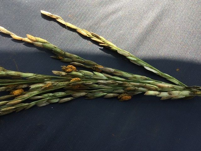
A PREPRINT - M AY 11, 2021

                                                                            Region
                                                Faster RCNN                Proposal
                                                                             Net
                                                                                                   Classification
                                                                                                       loss

                                                                 Feature
                                                                                       proposals
                                           Convolutional                                              BBox
                                             Layers               Map                               Regression
                                                                                                       loss

            input image

                Resized                                    Cropped

                                                                                                         Grain

               300 X 250                                                                           Phase 01

                                                                                      Class: Neck Blast             0.11

                                                                                      Class: False Smut             0.87

                                                                                        Class: Healthy              0.02

                                     CNN
                                                                                      Class: Neck Blast             0.79

                                                                                      Class: False Smut             0.16
              Phase 02
                                                                                        Class: Healthy              0.05

Figure 5: Proposed dual phase approach; Phase one for detection of the significant portion and phase two for
classification; A multiclass data have been presented as an example to demonstrate the classification strategy.

3.2     Proposed Dual Phase Approach

In this research, a dual phase approach has been introduced in order to learn effectively from small dataset containing
images with a lot of heterogeneity in the background. The approach overview has been provided in Figure. 5. In the
first phase, the original image is taken, reshaped to a fixed size and then passed through segmentation oriented Faster
RCNN architecture. At most two best regions have been selected from the first phase. After obtaining the significant
grain portions from an image, those regions are cropped and resized to a fixed size. These images look simple because
of the absence of heterogeneous background. CNN architecture is trained on this simplified dataset to detect disease.
The learning process has been showed to be effective through experiments.

3.2.1    Segmenting Grain Portion

This is the first phase of our approach. Segmentation algorithms based on CNN architecture as a backbone requires
image to be of fixed size. Input images have been resized to 640×480 before feeding them to Faster RCNN. The
consecutive stages of the network through which this resized image passes through have been described as follows.

                                                             6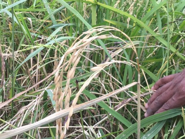
A PREPRINT - M AY 11, 2021

Convolutional Neural Network (CNN): In order to avoid sliding a window in each spatial position of the original
       image, CNN architecture is used in order to learn and extract feature map from the image which represents the
       image effectively. The spatial dimension of such feature map decreases whereas the channel number increases.
       For the dataset used in this research, VGG16 architecture has proven to be the most effective. Hence, VGG16
       has been used as the backbone CNN architecture which transforms the original image into 20 × 15 × 512
       dimension.
Region Proposal Network (RPN): The extracted feature map is passed through RPN layer. For each pixel of the
        feature map of spatial size 20×15, there are 16 possible bounding boxes (4 different aspect ratios and 4
        different sizes mentioned in bold letter in Table 2). So, that makes total 16×20×15 = 4800 possible bounding
        boxes, RPN is a two branch Convolution layer which provides two scores (branch one) and four coordinate
        adjustments (branch two) for each of the 4800 boxes. The two scores correspond to the probability of being
        an object and a non-object. Only those boxes which have a high object probability are taken into account.
        Non-max suppression (NMS) is used in order to eliminate overlapping object bounding boxes and to keep only
        the high probability unique boxes. The threshold of this overlap in this case is 0.8 IoU. From this probable
        object proposals, top 200 proposals according to object probability are passed to the next layers.
ROI Pooling: Each of the 200 selected object proposals correspond to some region in the CNN feature map. For
       passing each of these regions on to the dense layers of the architecture, each of the regions need to be of fixed
       size. ROI pooling layer takes each region and turns them into 7×7×512 using bilinear interpolation and max
       pooling.
RCNN Layer: RCNN layer consists of fully connected dense layers. Each of the 7×7×512 size feature maps are
      flattened and passed through these fully connected layers. The final layer has two branches. Branch one
      predicts if the input feature map is background class or significant grain portion. Branch two provides four
      regression values denoting the adjustment of the bounding box to better fit the grain portion. For each feature
      map, if the probability of being a grain is over 0.6, only then is the feature map considered as a probable
      grain portion and the adjusted coordinates are mapped to the original image in order to get the localized grain
      portion. The overlapping boxes are eliminated using NMS. The remaining bounding box regions are the
      significant grain portions.
Loss Function: The trainable layers of Faster RCNN architecture are: CNN backbone, RPN layer and RCNN layer. A
       loss function is needed in order to train these layers in an end to manner which is as follows.

                                                  1 X                         1 X ∗
                                 L(pi , ti ) =          Lcls (pi , p∗i ) + λ        p Lreg (ti , t∗i )
                                                 Ncls i                      Nreg i i

          The first term of this loss function defines the classification loss over two classes which describe whether
          predicted bounding box i is an object or not. The second term defines the regression loss of the bounding box
          when there is a ground truth object having significant overlap with the box. Here, pi and ti denote predicted
          object probability of bounding box i and predicted four coordinates of that box respectively while p∗i and t∗i
          denote the same for the ground truth bounding box which has enough overlap with predicted bounding box
          i. Ncls is the batch size (256 in this case) and Nreg is the total number of bounding boxes having enough
          overlap with ground truth object. Both these terms work as normalization factor. Lcls and Lreg are log loss
          (for classification) and regularized loss (for regression) function respectively.

3.2.2    Disease Detection from Segmented Grain
Figure. 5 shows Faster RCNN architecture drawing bounding boxes on two significant grain portions. These portions
are cropped and resized to a fixed size (300×250 in this case) in order to pass each of them through a CNN architecture.
Thus two images have been created from single image of the primary dataset. The same process can be executed on
each of the images of the primary dataset. Thus a secondary dataset of significant grain portion can be created. Each
of these images have to be labeled as one of the three classes in order to train the CNN architecture. The complete
dataset including these secondary image counts has been shown in Table 3. The cropped portions when passed through
a trained CNN model have been predicted as False Smut disease and Neck Blast class in Figure. 5 as it is an example of
multiclass data.

3.3     Evaluation Metric

All results have been provided in terms of 5 fold cross validation. Accuracy metric has been utilized in order to compare
dual phase approach against implementation of CNN on original images without any segmentation. Accuracy is a
suitable metric for balanced dataset.

                                                               7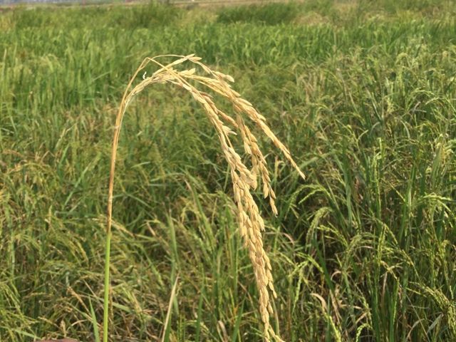
A PREPRINT - M AY 11, 2021

                                                           Image Count              Image
                                          Class
                                                       Primary Secondary            Increment
                                          False Smut 75          85                 10
                                          Neck Blast 63          70                 7
                                          Healthy      62        64                 2
                                          Total        200       219                19
                                                    Table 3: Complete Dataset

                                                                     TP         2
                                               Accuracy =
                                                              TP + FP + TN + FN
Segmenting the grain portion is the goal of the first phase of the dual phase approach. For evaluating the performance
of this phase, mAP (mean average precision) score has been used. Precision, recall and IoU (Intersection over Union)
are required to calculate mAP score.

                                                                      TP
                                                       P recision =
                                                                    TP + FP
                                                                     TP
                                                         Recall =
                                                                  TP + FN
                                                                   AOI 3
                                                           IoU =
                                                                  AOU
If a predicted box IoU is greater than a certain predefined threshold, it is considered as TP. Otherwise, it is considered
as FP. (T P + F N ) is actually the total number of ground truth bounding boxes. Average precision (AP) is calculated
from the area under the precision-recall curve. If there are N classes, then mAP is the average AP of all these classes. In
this research, there is only one class of object in phase one, that is the significant grain portion class. So, here AP and
mAP are the same.
As the proposed method has two stages: segmentation and classification, failure in proper segmentation can leads to
classification failure. In this work, two stages are created as an intact pipeline so that outcome of the first stage directed
to the second stage as input. Detail about the procedure mentioned in Subsection 4.2.

4         Results and Discussion
As mentioned earlier, the proposed dual-phase approach has been performed in two steps. First, segmentation of the
grain parts and lastly the classification of the segmented parts. This experiment has been mentioned as the prime
experiment throughout the paper. To verify the performance of the prime experiment, different CNN architectures and
Faster RCNN has been employed separately. This part of the experiment has been mentioned as the counter experiment.
Individual counter experiments have been performed to analyze their performance with the respective phase of the
prime experiment.

4.1        Counter Experiments

Two counter experiments have been performed named, counter experiment 01 and 02. Counter experiment 01 is based
on various CNN architectures where the goal is to obtain the classification outcome from the primary dataset. Counter
experiment 02 is based on Faster RCNN underlying three selected CNN architectures which has been applied for both
classification and detection of the three classes.

4.1.1        Counter Experiment 01: CNN
This experiment has been conducted applying five different CNN architectures which were mentioned earlier in
Subsubsection 3.1.2. Three transfer learning approaches have been followed (which are freezed layer, fine tuning and
fine tuning + dropout) in this part utilizing imagenet pretrained models. At first, freezing layer approach has been
      2
          TP: True Positive, FP: False Positive, TN: True Negative, FN: False Negative
      3
          AOI: Area of intersection, AOU: Area of union (with respect to ground truth bounding box)

                                                                    8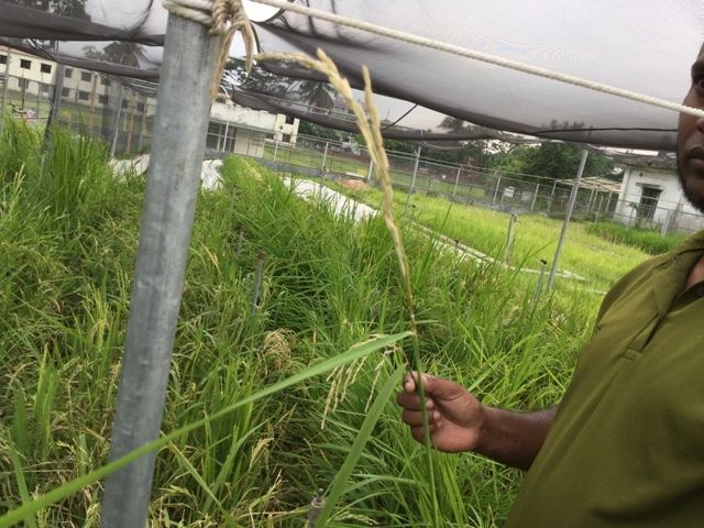
A PREPRINT - M AY 11, 2021

                                 Transfer                                Validation
                                                CNN                Validation
                                 learning                                Accuracy
                                                Architecture       Loss
                                 Approach                                (%)
                                              VGG16          2.08        63.33 ± 2.04
                                              VGG19          1.08        43.75 ± 3.43
                                 Freezed
                                              Xception       2.34        31.25 ± 4.04
                                  Layer
                                              InceptionV3 9.23           37.50 ± 3.89
                                              ResNet50       4.47        31.25 ± 3.27
                                              VGG16          2.71        67.79 ± 3.24
                                              VGG19          1.77        55.04 ± 3.00
                                  Fine
                                              Xception       6.29        43.76 ± 1.88
                                 Tuned
                                              InceptionV3 7.42           41.73 ± 3.66
                                              ResNet50       2.47        38.20 ± 1.34
                                              VGG16          3.47        69.43 ± 3.41
                                 Fine Tuned VGG19            3.11        57.18 ± 2.64
                                      +       Xception       5.72        47.17 ± 2.11
                                  Dropout     InceptionV3 4.12           48.22 ± 3.14
                                              ResNet50       2.81        42.31 ± 1.32
                                         Table 4: Counter Experiment 01: CNN

performed which is also known as a default transfer learning method. VGG16 outperformed other CNN architectures
with a validation accuracy of 63.33 ± 2.04 mentioned in Table 4. Then, finely-tuned approach has been applied which
shows improvement in validation accuracy of 67.79 ± 3.24 for VGG16. Finally, dropout has been applied inside the
CNN architectures which results in a significant improvement of 69.43 ± 3.41 for VGG16. Fine-tuning and fine-tuning
+ dropout have been performed several times by experimenting with dropout on various positions inside individual
CNNs. Although the standard deviation of the outcome for VGG16 is large which is an indication of low precision.
Comparative results for all five architecture have been shown in Table 4.

4.1.2    Counter Experiment 02: Faster RCNN

In this counter experiment 02, Faster RCNN has been applied utilizing three different CNN architectures as the
backbone. The goal of this experiment is to test the ability of Faster RCNN for efficient detection and classification
of the significant portion (grain). VGG16 and VGG19 have been chosen because of their performance at counter
experiment 01. Additionally, ResNet50 have chosen because of the lower validation loss than Xception and InceptionV3,
mentioned in Table 4. CNN models have been applied as pretrained model accumulated from COCO and Imagenet.
Different hyperparameter optimizations have been applied to reach the peak outcome for Faster RCNN mentioned in
Table 5.
Default settings from the Faster RCNN paper [31] for anchor box ratio were (1:1), (2:1), (1:2) and anchor box pixels
were 128, 256, 512. Which produces 3×3=9 anchor boxes per pixel. The default RPN threshold of (0.3 - 0.7), overlap
threshold 0.8 and default anchor box ratios and pixels, VGG16 (imagenet pretrained model) provided the best mAP
score of 71.0 ± 4.0. After tuning RPN threshold to (0.4 - 0.8), anchor box ratios to (1:1), ( √12 : √22 ), ( √22 : √12 ), (2:2)
and pixel sizes to 32, 64, 128, 256, 4×4=16 anchor boxes have been produced which provides better outcome than
before. This setting improved the mAP for VGG16 (imagent pretrained model) to 76.32 ± 2.29 which is the peak
outcome after several optimization.

4.2     Prime Experiment: Dual Phase Approach

Prime experiment has been performed by creating a pipeline in two phases shown in Figure. 5. In the first phase,
segmentations of grain has been performed and the segmented parts were cropped and saved as the secondary dataset,
mentioned in subsubsection 3.2.2. K fold cross-validation (K=5) have been performed where train and validation split
was 80:20. As a result, the full primary dataset has been converted into a secondary dataset. In the second phase, three
selected CNN architectures have been utilized for final classification after labelling the secondary dataset in terms of
three classes.

                                                               9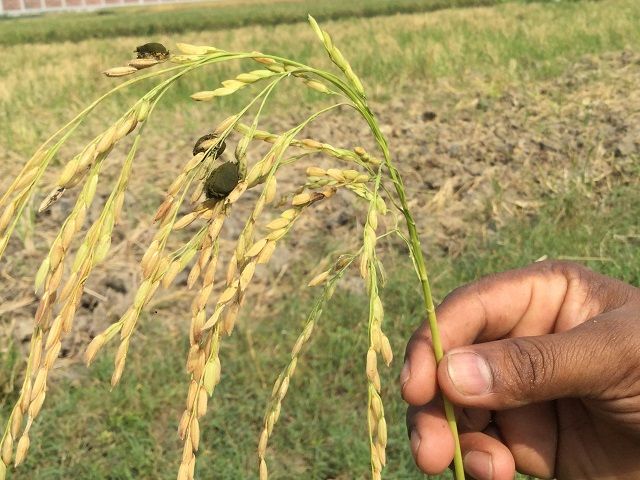
A PREPRINT - M AY 11, 2021

         Pretrained       Anchor            Anchor         RPN             CNN            Overlap
                                                                                                        mAP (%)
         Model            Box Ratio         Box Pixels     Threshold       Architecture   Threshold
                                                                           VGG16                        71.0 ± 4.0
                         (1:1), (2:1),      128,256,
                                                           0.3 - 0.7       VGG19          >0.8          47.06 ± 2.01
                            (1:2)             512
                                                                           ResNet50                     67.14 ± 6.68
                                                                                          >0.8          76.32 ± 2.29
                             (1:1),                                        VGG16
          Imagenet                                                                        >0.9          63.42 ± 2.36
                         ( √12 : √22 ),      32, 64,                                      >0.8          70.08 ± 4.54
                                                           0.4 - 0.8       VGG19
                         ( √22 : √12 ),     128, 256                                      >0.9          70.30 ± 2.36
                             (2:2)                                                        >0.9          40.02 ± 3.03
                                                                           ResNet50
                                                                                          >0.8          52.36 ± 5.91
                                                                           VGG16                        48.32 ± 4.79
                         (1:1), (2:1),      128,256,
                                                           0.3 - 0.7       VGG19          >0.8          32.30 ± 4.83
                            (1:2)             512
                                                                           ResNet50                     46.36 ± 2.04
                                                                                    >0.8                54.24 ± 2.23
                             (1:1),                                        VGG16
           COCO                                                                     >0.9                48.0 ± 2.10
                         ( √12 : √22 ),       32, 64,                               >0.8                42.36 ± 1.02
                                                          0.4 - 0.8   VGG19
                         ( √22 : √12 ),      128, 256                               >0.9                41.07 ± 5.21
                             (2:2)                                                  >0.9                28.42 ± 4.84
                                                                      ResNet50
                                                                                    >0.8                30.23 ± 3.0
                                          Table 5: Counter Experiment 02: Faster RCNN

                   grain: 91%                       grain:grain:
                                                           94% 91%
                 grain: 89%                                                                         grain: 94%

                 (a)                                                 (b)                                   (c)

Figure 6: Prime Experiment: First Phase; Sample Outcome: accuracy of detected objects. Phase One detected two
bounding boxes from (a) and (b) as the second bounding box meets IoU and accuracy threshold. (c) have not met the
IoU or accuracy threshold so the second bounding box is absent.

                                                                     10
A PREPRINT - M AY 11, 2021
Anchor Anchor RPN CNN Overlap
mAP (%)
Box Ratio Box Pixels Threshold Architecture Threshold
(1:1),( √12 : √22 ), VGG16 >0.8 84.3 ± 2.36
32, 64,
0.4 - 0.8 VGG19 >0.8 73.5 ± 1.34
( √22 : √12 ),(2:2)) 128, 256
ResNet50 >0.8 65.9 ± 2.59
Table 6: Prime Experiment: Phase One
Train Validation
CNN Train Validation
Accuracy Accuracy
Architecture Loss Loss
(%) (%)
VGG16 0.196 94.47 0.195 88.11 ± 3.86
VGG19 0.095 89.98 0.093 86.43 ± 2.98
ResNet50 0.367 89.63 0.281 78.00 ± 2.32
Table 7: Prime Experiment: Phase Two
4.2.1 Phase One: Segmentation of Grains
The goal of phase one is to crop out the significant part (grain) from a particular image. Faster RCNN have been
utilized following three different CNN architecture as the backbone. Applied CNN architectures were VGG16,
VGG19 and ResNet50 which were already applied in counter experiment 02 mentioned in Subsubsection 4.1.2. Also,
hyperparameters setting have been followed from the counter experiment 02. Only the best performed hyperparameter
setting were applied in phase one mentioned in Table 2. Faster RCNN with VGG16 as backbone achieved the best
mAP score of 84.3 ± 2.36. The result have been achieved through five fold cross validation. Thus all images in the
dataset have been evaluated. From each image at most two new images have been generated which creates a secondary
dataset. This operation has been performed by selecting two best bounding boxes from each image. First bounding box
is the best bounding box referred by the Faster RCNN which is cropped and became the part of the new dataset. Second
bounding box has been selected which satisfy the IoU threshold of 0.5 and accuracy threshold of 90%. For several
images there were no bounding boxes which met this requirement. On that case only one image have been selected for
the new dataset. Figure. 6 shows the bounding boxes from each image for phase one. Here on sub figure (c) only one
bounding box get detected.
4.2.2 Phase Two: Classification
Image data received from phase one channeled through phase two where it provides the classification result. Again
three different CNN architecture, VGG16, VGG19 and ResNet50 have been applied in this phase. Best settings from
counter experiment 01 have been reapplied in this phase that has been mentioned in Subsubsection 4.1.1. VGG16
emerged with the best validation accuracy of 88.11 ± 3.86 mentioned in Table 7.
Figure. 7 shows loss and accuracy graph for train and validation of the first training fold out of five folds for phase two.
The graphs also shows the training was less time consuming as the dataset was small. By zooming in the graph it is
visible that VGG16 was still learning shown in Figure. 8.
In general, expectancy from CNN models like VGG16 is higher in this dataset as there is only 3 class and they are quite
different from each other in terms of class features. This is a pipeline-based process and phase one can generate FP/FN
results which will be channeled through phase two. As a result, phase two will be unable not classify them properly.
Which is a limitation of this system. This issue can be solved by presenting a new class which can be titled "No Grain"
that will declare anything but grain.
5 Conclusion
In brief, this research has the following contributions:
– A dual phase approach capable of learning from small rice grain disease dataset has been proposed.
– A smart segmentation procedure has been proposed in phase one which is capable of handling heterogeneous
background prevalent in plant disease image dataset collected in real life scenario
– Experimental comparison has been provided with straightforward use of state-of-the-art CNN architectures on the
small rice grain dataset to show the effectiveness of the proposed approach.
11A PREPRINT - M AY 11, 2021
(a) (b) (c)
Figure 7: Accuracy and loss for train and validation; Phase Two.(a)VGG16, (b)VGG19, (c)ResNet50.
(a) (b) (c)
Figure 8: Accuracy and loss for train and validation (Zoomed); Phase Two. Only VGG 16 is showing further
improvement is possible through training.(a)VGG16, (b)VGG19, (c)ResNet50.
12A PREPRINT - M AY 11, 2021
6 Acknowledgments
We thank Information and Communications Technology (ICT) division, Bangladesh for aiding this research and the
authority of Bangladesh Rice Research Institute (BRRI) for supporting us with field level data collection. We also
acknowledge the help of RMIT University who gave us the opportunity to use their GPU server.
References
[1] Mathew S Baite, S Raghu, SR Prabhukarthikeyan, U Keerthana, Nitiprasad N Jambhulkar, and Prakash C Rath.
Disease incidence and yield loss in rice due to grain discolouration. Journal of Plant Diseases and Protection,
pages 1–5, 2019.
[2] MM Atia. Rice false smut (ustilaginoidea virens) in egypt. Journal of Plant Diseases and Protection, 111(1):71–82,
2004.
[3] Shu Huang Ou. Rice diseases. IRRI, 1985.
[4] Mohammad Ashik Iqbal Khan, Md Rejwan Bhuiyan, Md Shahadat Hossain, Partha Pratim Sen, Anjuman Ara,
Md Abubakar Siddique, and Md Ansar Ali. Neck blast disease influences grain yield and quality traits of aromatic
rice. Comptes rendus biologies, 337(11):635–641, 2014.
[5] BODRUN Nessa. Rice False Smut Disease in Bangladesh: Epidemiology, Yield Loss and Management. PhD
thesis, PhD thesis, Department of Plant Pathology and Seed Science, Sylhet . . . , 2017.
[6] Reinald Adrian DL Pugoy and Vladimir Y Mariano. Automated rice leaf disease detection using color image
analysis. In Third International Conference on Digital Image Processing (ICDIP 2011), volume 8009, page
80090F. International Society for Optics and Photonics, 2011.
[7] Prabira Kumar Sethy, Baishalee Negi, and Nilamani Bhoi. Detection of healthy and defected diseased leaf of rice
crop using k-means clustering technique. International Journal of Computer Applications, 157(1):24–27, 2017.
[8] Chia-Lin Chung, Kai-Jyun Huang, Szu-Yu Chen, Ming-Hsing Lai, Yu-Chia Chen, and Yan-Fu Kuo. Detecting
bakanae disease in rice seedlings by machine vision. Computers and electronics in agriculture, 121:404–411,
2016.
[9] Taohidul Islam, Manish Sah, Sudipto Baral, and Rudra RoyChoudhury. A faster technique on rice disease
detectionusing image processing of affected area in agro-field. In 2018 Second International Conference on
Inventive Communication and Computational Technologies (ICICCT), pages 62–66. IEEE, 2018.
[10] MN Abu Bakar, AH Abdullah, N Abdul Rahim, H Yazid, SN Misman, and MJ Masnan. Rice leaf blast disease
detection using multi-level colour image thresholding. Journal of Telecommunication, Electronic and Computer
Engineering (JTEC), 10(1-15):1–6, 2018.
[11] MS Prasad Babu, B Srinivasa Rao, et al. Leaves recognition using back propagation neural network-advice for
pest and disease control on crops. IndiaKisan. Net: Expert Advisory System, 2007.
[12] Santanu Phadikar and Jaya Sil. Rice disease identification using pattern recognition techniques. In 2008 11th
International Conference on Computer and Information Technology, pages 420–423. IEEE, 2008.
[13] Ronnel R Atole and Daechul Park. A multiclass deep convolutional neural network classifier for detection of
common rice plant anomalies. INTERNATIONAL JOURNAL OF ADVANCED COMPUTER SCIENCE AND
APPLICATIONS, 9(1):67–70, 2018.
[14] Yang Lu, Shujuan Yi, Nianyin Zeng, Yurong Liu, and Yong Zhang. Identification of rice diseases using deep
convolutional neural networks. Neurocomputing, 267:378–384, 2017.
[15] Mohammed Brahimi, Kamel Boukhalfa, and Abdelouahab Moussaoui. Deep learning for tomato diseases:
classification and symptoms visualization. Applied Artificial Intelligence, 31(4):299–315, 2017.
[16] Chowdhury Rafeed Rahman, Preetom Saha Arko, Mohammed Eunus Ali, Mohammad Ashik Iqbal Khan,
Sajid Hasan Apon, Farzana Nowrin, and Abu Wasif. Identification and recognition of rice diseases and pests using
convolutional neural networks. arXiv preprint arXiv:1812.01043, 2018.
[17] Konstantinos P Ferentinos. Deep learning models for plant disease detection and diagnosis. Computers and
Electronics in Agriculture, 145:311–318, 2018.
[18] Jayme Garcia Arnal Barbedo. Impact of dataset size and variety on the effectiveness of deep learning and transfer
learning for plant disease classification. Computers and electronics in agriculture, 153:46–53, 2018.
13A PREPRINT - M AY 11, 2021
[19] Jitesh P Shah, Harshadkumar B Prajapati, and Vipul K Dabhi. A survey on detection and classification of rice
plant diseases. In 2016 IEEE International Conference on Current Trends in Advanced Computing (ICCTAC),
pages 1–8. IEEE, 2016.
[20] D Amutha Devi and K Muthukannan. Analysis of segmentation scheme for diseased rice leaves. In 2014 IEEE
International Conference on Advanced Communications, Control and Computing Technologies, pages 1374–1378.
IEEE, 2014.
[21] Raymond Liu and Duncan F Gillies. Overfitting in linear feature extraction for classification of high-dimensional
image data. Pattern Recognition, 53:73–86, 2016.
[22] Connor Shorten and Taghi M Khoshgoftaar. A survey on image data augmentation for deep learning. Journal of
Big Data, 6(1):60, 2019.
[23] Michael Cogswell, Faruk Ahmed, Ross Girshick, Larry Zitnick, and Dhruv Batra. Reducing overfitting in deep
networks by decorrelating representations. arXiv preprint arXiv:1511.06068, 2015.
[24] Richard A Wilson and Nicholas J Talbot. Under pressure: investigating the biology of plant infection by
magnaporthe oryzae. Nature Reviews Microbiology, 7(3):185–195, 2009.
[25] Yukiko Koiso, YIN Li, Shigeo Iwasaki, KENJI HANAKA, Tomowo Kobayashi, Ryoichi Sonoda, Yoshikatsu
Fujita, Hiroshi Yaegashi, and Zenji Sato. Ustiloxins, antimitotic cyclic peptides from false smut balls on rice
panicles caused by ustilaginoidea virens. The Journal of antibiotics, 47(7):765–773, 1994.
[26] SA Miah, AKM Shahjahan, MA Hossain, and NR Sharma. A survey of rice diseases in bangladesh. International
Journal of Pest Management, 31(3):208–213, 1985.
[27] Karen Simonyan and Andrew Zisserman. Very deep convolutional networks for large-scale image recognition.
arXiv preprint arXiv:1409.1556, 2014.
[28] Kaiming He, Xiangyu Zhang, Shaoqing Ren, and Jian Sun. Deep residual learning for image recognition. In
Proceedings of the IEEE conference on computer vision and pattern recognition, pages 770–778, 2016.
[29] Christian Szegedy, Vincent Vanhoucke, Sergey Ioffe, Jon Shlens, and Zbigniew Wojna. Rethinking the inception
architecture for computer vision. In Proceedings of the IEEE conference on computer vision and pattern
recognition, pages 2818–2826, 2016.
[30] François Chollet. Xception: Deep learning with depthwise separable convolutions. In Proceedings of the IEEE
conference on computer vision and pattern recognition, pages 1251–1258, 2017.
[31] Shaoqing Ren, Kaiming He, Ross Girshick, and Jian Sun. Faster r-cnn: Towards real-time object detection with
region proposal networks. In Advances in neural information processing systems, pages 91–99, 2015.
14You can also read