ESTIMATED ABUNDANCES OF CETACEAN SPECIES IN THE NORTHEAST ATLANTIC FROM NORWEGIAN SHIPBOARD SURVEYS CONDUCTED IN 2014-2018 - Septentrio Academic ...
←
→
Page content transcription
If your browser does not render page correctly, please read the page content below
ARTICLE
NAMMCO Scientific Publications

ESTIMATED ABUNDANCES OF CETACEAN SPECIES IN THE
NORTHEAST ATLANTIC FROM NORWEGIAN SHIPBOARD SURVEYS
CONDUCTED IN 2014–2018
Deanna M. Leonard1,2 & Nils I. Øien1
1 IMR   - Institute of Marine Research, Bergen, Norway. Corresponding author: deanna.leonard@hi.no
2 NAMMCO        - North Atlantic Marine Mammal Commission, Tromsø, Norway

                                                                   ABSTRACT

A ship-based mosaic survey of Northeast Atlantic cetaceans was conducted over a 5-year period between 2014–2018. The area
surveyed extends from the North Sea in the south (southern boundary at 53oN), to the ice edge of the Barents Sea and the Greenland
Sea. Survey vessels were equipped with 2 independent observer platforms that detected whales in passing mode and applied tracking
procedures for the target species, common minke whales (Balaenoptera acutorostrata acutorostrata). Here we present abundance
estimates for all non-target species for which there were sufficient sightings. We estimate the abundance of fin whales (Balaenoptera
physalus) to be 11,387 (CV=0.17, 95% CI: 8,072–16,063), of humpback whales (Megaptera novaeangliae) to be 10,708 (CV=0.38, 95%
CI: 4,906–23,370), of sperm whales (Physeter macrocephalus) to be 5,704 (CV=0.26, 95% CI: 3,374–9,643), of killer whales (Orcinus
orca) to be 15,056 (CV=0.29, 95% CI: 8,423–26,914), of harbour porpoises (Phocoena phocoena) to be 255,929 (CV=0.20, 95% CI:
172,742–379,175), dolphins of genus Lagenorhynchus to be 192,767 (CV=0.25, 95% CI: 114,033–325,863), and finally of northern
bottlenose whales (Hyperoodon ampullatus) to be 7,800 (CV=0.28, 95% CI: 4,373–13,913). Additionally, our survey effort in the
Norwegian Sea in 2015 contributed to the 6th North Atlantic Sightings Survey (NASS) and the survey was extended into the waters
north and east of Iceland around Jan Mayen island. This NASS extension, along with our Norwegian Sea survey in 2015, was used to
estimate the abundance of fin whales, humpback whales, and sperm whales. All estimates presented used mark-recapture distance
sampling techniques and were thus corrected for perception bias. Our estimates do not account for additional variance due to
distributional shifts between years or biases due to availability or responsive movement.
Keywords: North Atlantic, cetacean, abundance, line-transect, fin whales, humpback whales, sperm whales, killer whales, harbour porpoises, dolphins,
northern bottlenose whales

INTRODUCTION

Norwegian shipboard line-transect surveys of the Northeast                   whales     (Hyperoodon      ampullatus),      and      dolphins
Atlantic have been ongoing since 1987 as part of a program to                (Lagenorhynchus spp). Throughout this paper, the term
estimate abundance of common minke whales (Balaenoptera                      Lagenorhynchus spp. refers collectively to white-sided dolphins
acutorostrata acutorostrata) as input to the Revised                         (Lagenorhynchus acutus) and white-beaked dolphins
Management Procedure (RMP) of the International Whaling                      (Lagenorhynchus albirostris), which are estimated to genus,
Commission (IWC, 1994). All non-target cetacean species are                  rather than species level.
also documented throughout the surveys. In 1995, a full
                                                                             In addition to providing information for the management of
synoptic survey of the study area (described under Materials
                                                                             whaling under the RMP, the survey in 2015 also contributed to
and Methods) was completed, prior to which only subsets of the
                                                                             the synoptically conducted North Atlantic Sightings Survey
total study area were surveyed. The current multi-year mosaic
                                                                             (NASS). In collaboration with the North Atlantic Marine
survey design was introduced in 1996 as a way of providing
                                                                             Mammal Commission (NAMMCO), survey blocks around Jan
complete coverage of the study area with smaller-scale effort
                                                                             Mayen were added to the planned 2015 survey to create
each year (Øien & Schweder 1996). To date, 4 complete cycles
                                                                             continuous survey coverage from areas around Iceland
of the multi-year program have been completed (1996–2001,
                                                                             extending north to the Jan Mayen region and westward
2002–2007, 2008–2013, 2014–2018). Abundance estimates of
                                                                             covering the Norwegian Sea. The areas to the south and west of
non-target species have been published from surveys
                                                                             Jan Mayen were surveyed simultaneously by 3 Icelandic and
conducted in 1988, 1989, 1995 (Christensen et al., 1992; Øien
                                                                             Faroese vessels. Results from the analysis of data from these
1990, 2009), and the mosaic surveys in 1996–2001, 2002–2007
                                                                             surveys are presented in Pike et al. (2019).
and 2008–2013 (Øien 2009; Leonard & Øien, 2020). This paper
presents new abundance estimates from the 2014–2018 mosaic                   The design of Norwegian line-transect surveys for minke whales
survey for all cetacean species for which there were a sufficient            has remained consistent since 1995, with slight changes to
number of sightings. This includes fin whales (Balaenoptera                  improve the precision of the abundance estimates (Schweder,
physalus), humpback whales (Megaptera novaeangliae), sperm                   Skaug, Dimakos, Langaas, & Øien, 1997; Skaug, Øien, Schweder,
whales (Physeter macrocephalus), killer whales (Orcinus orca),               & Bøthun, 2004). For example, beginning in 2008, a plan to
harbour porpoises (Phocoena phocoena), northern bottlenose                   survey each Small Management Area (SMA – as defined by the

Leonard, D. M. & Øien, N. I. (2020). Estimated Abundances of Cetacean Species in the Northeast Atlantic from Norwegian Shipboard Surveys Conducted
in 2014–2018. NAMMCO Scientific Publications 11. https://doi.org/ 10.7557/3.4694

                                                                                                     Creative Commons License
Leonard & Øien (2020)
RMP) in a single year was implemented to reduce additional Data collection
variance caused by distributional shifts of minke whales
Throughout the survey cycle, one vessel operated alone,
between years (Skaug et al., 2004). A modification was made to
starting in mid-June and ending in mid-August in each of the 5
the data collection in this 2014–2018 cycle, which involved
survey years. In 2014, the Svalbard area was surveyed; in 2015
assigning confidence ranking to each duplicate judgement for
the Norwegian Sea and NASS extension blocks (see below); in
all species to allow for a sensitivity analysis. Some of the analysis
2016 the Jan Mayen area; in 2017 the Barents Sea; and in 2018
methods have also changed since the earlier surveys. Standard
the North Sea was surveyed as well as a small block of the
distance sampling methods were used to estimate the
Norwegian Sea (EW4).
abundances of non-target species from data collected in 1995
and 1996–2001 (Christensen et al., 1992; Øien, 2009, 1990). All Each vessel was outfitted with 2 survey platforms that were
later surveys (2002–2007, 2008–2013, including the current visually and audibly separated to facilitate observer
survey) have used mark-recapture distance sampling methods independence. Each platform operated with 2 observers
applied to combined-platform data to correct for perception searching forward 45o from 0o (centre of the bow) on either the
bias in the estimates. starboard or port side. The lower platform, platform 2, was
positioned on the wheelhouse roof and the upper platform,
MATERIALS AND METHODS referred to as platform 1, was typically placed in the barrel on
the mast of the ship. The height of the platforms varied
between vessels, with eye-height above sea level averaged 13.8
Survey Design m for platform 1 and 9.7 m for platform 2 (Figure 2). Four 2-
person teams of observers operated in 1- to 2-hour shifts,
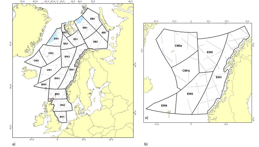
The study area extended from the North Sea in the south, with
rotating between platforms.
a southern boundary at 53oN, to the ice edge of the Barents Sea
and the Greenland Sea in the north (Figure 1a) and comprised Observers recorded sightings nearly instantaneously using a
the Small Management Areas (SMA), as revised by the North microphone connected to GPS-equipped computer system,
Atlantic Minke Whale Implementation in 2003 (IWC, 2004). The monitored on the bridge. The species, radial distance, angle
five SMAs were CM, ES, EB, EW, and EN. The survey block from the transect line, and group size were recorded for each
structure was defined within the SMAs using previous sighting. The search method was by naked eye, angles were
knowledge of minke whale density to minimize within-block read from an angle board, and radial distances were estimated
variation. Transects within each block were constructed as zig- without equipment. Observers were trained to estimate
zag tracks with a random starting point, with survey effort distances through exercises conducted during the surveys using
distributed proportional to area (Buckland et al., 2001). buoys as targets.
Calculated block areas were adjusted for ice-cover.
Specific tracking procedures were followed for minke whale
The 2015 survey area consisted of 6 blocks (Figure 1b) and was sightings, where each surfacing was recorded until the whale
conducted over the period of 22 June to 30 August. The NASS passed the ship’s abeam. For all other species, only the first
extension blocks (CM) were surveyed from 13 July to 2 August. sighting was recorded, with occasional updates to species
Figure 1. (a) Survey blocks (derived from minke whale SMAs) and realized search effort on predetermined transect lines during the 2014–2018 sighting
surveys, with the blue areas representing ice coverage; (b) the 2015 NASS extension survey blocks and transects.
NAMMCO Scientific Publications, Volume 11 2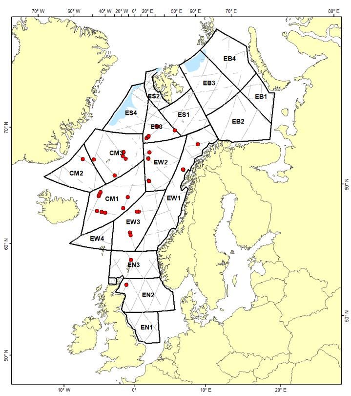
Leonard & Øien (2020)

identification and position information to aid in judging              The effect of duplicate identification uncertainty was explored
duplicates. Dolphin groups were often recorded as                      by assigning each duplicate judgement a confidence level of ‘D’
Lagenorhynchus spp. and not identified to species level. Large         for definite (high confidence), ‘P’ for probable (medium
whales that were not identified to species level were recorded         confidence), and ‘R’ for remote (low confidence). This allowed
as ‘unidentified large whales’. After each completed recording         for comparison of the resulting abundance estimates to
of a minke whale or other large whale sighting, observers              determine the influence of variation in identifying duplicates.
reported the sighting to the team leader by radio. The platforms
                                                                       The analytical method used required that the perpendicular
operated on separate radio channels to maintain
                                                                       distance and group size fields be identical for duplicate sightings
independence. The team leader, operating from the bridge,
                                                                       (Laake & Borchers, 2004). Thus, information recorded by the
assisted with species identification by using binoculars to
                                                                       platform from which the whale was first sighted was used.
confirm uncertain identifications.
                                                                       Analysis
                                                                       Sightings used in the analyses were all initially detected before
                                                                       coming abeam of the ship and recorded from platform 1, 2 or
                                                                       both. Only sightings that were identified to species by at least
                                                                       one platform were used in the estimates (with the exception of
                                                                       dolphins, which were estimated by genus (Lagenorhynchus
                                                                       spp.)).
                                                                       Data analyses were carried out using the DISTANCE 7.2 software
                                                                       package (Thomas et al., 2010). Density and abundance were
                                                                       estimated using mark-recapture distance sampling (MRDS)
                                                                       techniques (Laake & Borchers, 2004). The mark-recapture
                                                                       method uses the double-platform configuration to estimate
                                                                       p(0) to account for sightings that are missed (perception bias),
                                                                       rather than assume that all animals on the transect line are
                                                                       detected (p(0)=1), as with standard distance sampling methods
                                                                       (Thomas et al., 2010). The “independent observer
                                                                       configuration” was used because the platforms were fully
                                                                       independent of each other (Laake & Borchers, 2004). Two levels
                                                                       of independence were tested and selected based on a
                                                                       comparison of the AIC values: “full independence” (FI) and
                                                                       “point independence” (PI). The full independence method
Figure 2. Platform 1 (upper) and platform 2 (lower) aboard the ACC
                                                                       treats sightings as independent at all perpendicular distances
Mosby. Photo credit: Deanna Leonard
                                                                       and requires a conditional detection function (Mark Recapture
                                                                       model: MR model) to estimate detection probabilities
All survey effort was conducted at a speed of 10 knots at a
                                                                       conditioned on detection by the other platform. The
Beaufort Sea State (BSS) of 4 or less with visibility greater than
                                                                       assumption of point independence treats sightings as
1 km. On an hourly basis and as conditions changed, the
                                                                       independent on the trackline only (Laake & Borchers, 2004) and
weather conditions, BSS, visibility, and glare were recorded.
                                                                       requires a second detection function: one for the probability of
More detail on the survey design, observer protocols, and
                                                                       detection by one or more observers (Distance Sampling model:
covariate classification is provided in Øien (1995).
                                                                       DS model) in addition to the conditional detection function (MR
Data treatment                                                         model). The conditional detection function is modelled as a
                                                                       Generalized Linear Model (GLM) with a log link function.
The sightings from each platform were combined to constitute
a single dataset. When possible, duplicate sightings were              Detection functions were fitted using sightings pooled over all
identified in real time by a team leader operating from the            blocks for each species. Hazard-rate and half-normal models
bridge, however most were determined post-cruise. Sightings            were explored, and the sightings were truncated by 5-10% of
were judged as duplicates based on species identification,             the overall distance if it improved the Q-Q plot and goodness of
group size, and sighting location, considering the time between        fit metrics (Kolmogorov-Smirnov or Cramer-von-Mises test
the sightings and the relative position to the vessel while            statistics). Models were tested with candidate covariates
accounting for the vessel track and speed, allowing for small          including BSS, vessel identity, weather code, group size, glare,
differences in recorded radial distances. Due to the absence of        and visibility. Some covariates were simplified by aggregating
tracking procedures for non-target species, there was                  values or levels, as described in Table 1, to improve model fit.
occasionally the need to match duplicates of disparate                 Covariates were added to the detection functions through the
surfacings of the same whale. The team leader played an                scale parameter in the key function, and thus affected the scale
important role in identifying these duplicates in the field. When      but not the shape of the detection curve (Thomas et al., 2010).
only one platform reported a sighting, the team leader could           Model selection was achieved through visual inspection
track the whale so that it could be identified as a duplicate if the   (especially of data around the transect line), goodness of fit test
other platform detected it closer to the ship. In rare instances       statistics, and by minimizing Akaike’s information criterion
where one observer of an obvious duplicate sightings pair              (AIC). Covariates were retained only if their inclusion resulted in
identified the species, while the other recorded it as an              a lower AIC value when compared to base models.
‘unidentified large whale’, the positive ID was used.

NAMMCO Scientific Publications, Volume 11                                                                                               3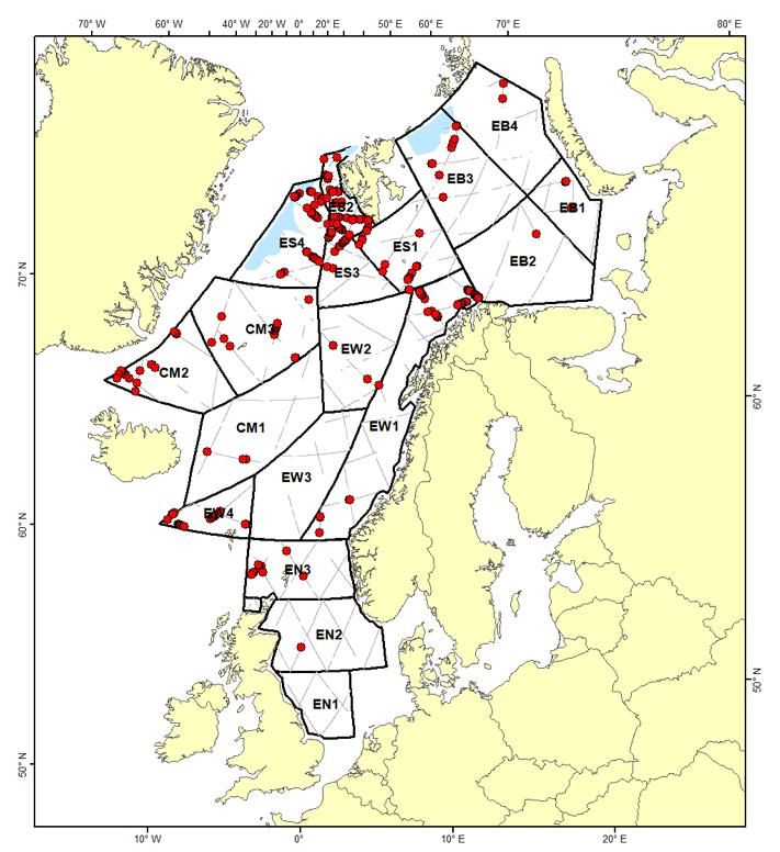
Leonard & Øien (2020)

Table 1. Descriptions of covariates included to improve model fit. Some covariates were aggregated into levels for simplification.

                                                                                                 Aggregated Covariates
  Covariate               Description                Symbol                      Levels                              Definition

  Beaufort                5 categories                   B                       BI, BII, BIII                       BI: [0–1], BII: [2], BIII: [3-4]

                                                                                                                     good: W01–W04, bad: W05–
  Weather                 12 categories                  W                       good, bad
                                                                                                                     W12
                                                        Ves
  Vessel                  3 vessels                                                       -                                           -

                                                                                                                     low < 50% of Max
  Visibility              numerical                      V                       high, low
                                                                                                                     high > 50% of Max
                                                         G
  Glare                   4 categories                                           glare, no glare                     G0: no glare, G1: glare

  Group size              numerical                      S                                -                                           -

  Distance                numerical                      D                                -                                           -

Estimates of density, abundance, and group size for each                       435 as harbour porpoises, 461 as Lagenorhynchus spp., 27 as
species were estimated by block, and the effective search half                 northern bottlenose whales and 11 as pilot whales.
width (eshw) was estimated globally. Encounter rate variances
                                                                               In all cases, the PI models resulted in lower AICs than the FI
were estimated by weighting transect lines by length using a
                                                                               models, therefore the PI method was accepted as superior. The
design-based empirical estimator (Fewster et al., 2009) from
                                                                               fitted covariates for each species, for both the Distance
the mark-recapture distance sampling (MRDS) engine in
                                                                               Sampling models (DS model) and the Mark Recapture models
DISTANCE 7.2 (Buckland et al., 2001).
                                                                               (MR model), are detailed in Table 3.
In 2015, the NASS extension blocks (CM3a, CM1a) were added
                                                                               A comparison of estimates using 3 levels of confidence in
to the regularly planned survey effort (EW blocks) to create a
                                                                               duplicate judgement showed no significant difference (p>0.05)
continuous expansion of the NASS survey covering the Jan
                                                                               between the estimates of p(0) and resulting abundance when
Mayen region and the Norwegian Sea. The 2015 effort and
                                                                               using D+P+R duplicates or D+P duplicates, but substantial
sightings were used to fit detection functions and produce
                                                                               differences when only D duplicates were used (Table 4). Using
estimates separate from the regular 2014–2018 survey.
                                                                               only D duplicates resulted in a 5–45% decrease in p(0) and
Abundances were estimated for 3 large whale species: fin
                                                                               proportional increase in the resulting abundance estimates
whales, humpback whales, and sperm whales. Data from the
                                                                               (Table 4). The differences were significant (p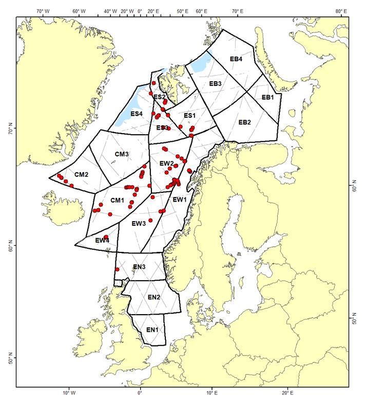
Leonard & Øien (2020)

Figure 3. Distribution of sightings recorded as fin whales during the          Figure 5. Distribution of sightings recorded as humpback whales during
2014–2018 sighting surveys. The blue areas represent ice coverage.             the 2014–2018 sighting surveys. The blue areas represent ice coverage.

Humpback whales                                                                Sperm whales
Humpback whales were sighted in 3 key areas: the northern                      Sperm whale sightings occurred over the deep waters of the
Barents Sea (EB3); around Bear Island (ES1); and north and east                Norwegian Sea (EW2), south of Jan Mayen (CM1) (Table 8;
of Iceland (CM2, CM3). Figure 5 shows the distribution of                      Figure 6). The data were truncated at a perpendicular distance
humpback whale sightings. The DS detection function was fitted                 of 4000 m and fitted with a half-normal DS detection function,
with a hazard-rate key function to data truncated at a distance                resulting in an estimated p(0)=0.69 (CV=0.15) and eshw of 1849
of 3000 m, which resulted in an estimated p(0)=0.76 (CV=0.07)                  m. The fitted DS detection function and MR conditional
and eshw of 1087 m. Figure 4b illustrates the fitted DS detection              detection function are shown in Figure 4c. Total corrected
function and conditional detection function (MR model). Total                  abundance of sperm whales was estimated to be 5,704
corrected abundance of humpback whales was estimated to be                     (CV=0.26, 95% CI: 3,374–9,643) (Table 8).
10,708 (CV=0.38, 95% CI: 4,906–23,370). Abundance and
density estimated by survey block are detailed in Table 7.

Figure 4. Detection function curves for pooled detections (top) and the conditional detection probabilities of platform 1 (bottom) for (a) fin whales,
(b) humpback whales, and (c) sperm whales.

NAMMCO Scientific Publications, Volume 11                                                                                                                5
Leonard & Øien (2020)

 Table 2. Summary of effort and sightings for each species, survey block, and year. The NASS extension survey blocks are shaded grey and excluded from the summed totals.

                                           Total                                                                                                                                N.
                             Area                     Large       Fin        Humpback      Sperm        Blue       Sei        Killer     Lag.        Harbour     Pilot                   Bowhead
     Year       Block                    Transect                                                                                                                           bottlenose                  Total
                            sq. km                    whales     whales       whales       whales      whales     whales     whales      spp.       porpoises   Whales                    whales
                                          length                                                                                                                             whales

                ES1         175,488          1,629          8         24             12         10                                         116                                                              170
                ES2          53,341          1,594         10         44              1           3          2                               76                                                             136
    2014
                ES3         118,763          1,359          3         31                        10                                10         53                                                             107
                ES4         141,180          1,195          2         46              2          1           1          1                     2                                                              55
                EW1         333,180          2,682          8         58             12           8                                3         44           12                                                145
                EW2         218,943          1,339          4          2              3         23                                 9                                                                            41
    2015        EW3         228,406          1,001          1                                     4                                5            2                                                               12
               CM1a         163,337            622                     1                        13                                              1                                                               15
               CM3a         295,796          1,772          2          7              2           3          3                                  8                                   2                           27
                CM1         297,396          1,611                     3                        25                                11            1                     4             4                           48
    2016        CM2         177,961          1,220          7         19              7           7          5                     1            1                                   6                           53
                CM3         295,929          1,481          4         15              9           1          2                     7            1                                  13                           52
                EB1         107,105            971          1          3             12                                                      17           23                                                    56
                EB2         278,964          1,236          2          1                                                                     62           37                                                102
    2017
                EB3         232,370          1,792          4         13             40                                                      36           25                                                118
                EB4         233,900            938          5          4                                                                        3         10                                    5               27
                EW4          84,625            861                    24                                                1                       2          7          4             4                           42
                EN1          95,675          1,027                                                2                                             4         92                                                    98
    2018
                EN2         197,293          2,124          1          1                                                                     23          138                                                163

                EN3         160,660          1,504          4         10                                                                     18           91          3                                     126

    Total                 3,431,179         25,564         64        298             98         94         10           2         46       461           435         11            27           5           1551

NAMMCO Scientific Publications, Volume 11                                                                                                                                                           6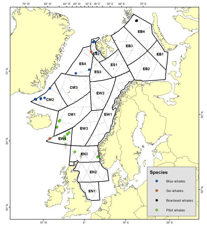
Leonard & Øien (2020)

      Table 3. Covariates included in the final models for each species for the                             Table 5. The total number of sightings (n), sightings by platform, and duplicate sighting for each species using
      distance sampling model (DS model) and the conditional detection function                             definite + probable (D+P) duplicates.
      (mark recapture or MR model). Distance (D) is automatically added as a
      covariate in the DS model. B=Beaufort Sea State, W=weather, Ves=vessel,                                                                                                Sightings (D+P)
      V=visibility, G=glare, S=group size, D=distance.
                                                                                                              Species
                                                                                                                                                            n        Platform 1    Platform 2              Duplicates
                                                 Covariates                                                   Fin whales                                   294          225          197                    128
                                                                                                              Humpback whales                               99           69           64                     34
       Species                            DS Model       MR Model
       Fin whales                         W                                                                   Sperm whales                                  94           74           56                     36
       Humpback whales                                                                                        Harbour porpoises                            443          261          284                    102
       Sperm whales                       W                     D                                             Killer whales                                 47           37           33                     23
       Harbour porpoises                  B                     B+D+S                                         Lagenorhynchus spp.                          426          303          316                    193
       Killer whales                      S                                                                   N. bottlenose whales                          36           25           27                     16
       Lagenorhynchus spp.                B+S                   D                                             NASS Extension (2015)
       N. bottlenose whales                                                                                   Fin whales                                    68              55              39                  26
                                                                                                              Humpback whales                               17              14              10                   7
       NASS Extension (2015)
                                                                                                              Sperm whales                                  51              38              32                  19
       Fin whales                         B                     D
       Humpback whales                    W                     D
       Sperm whales

         Table 4. Estimated p(0) and corresponding abundance estimates using 3 combinations of duplicates: definite (D), definite + probable (D+P), and definite + probable + remote (D+P+R).

                                                                 D+P+R                                                    D+P                                                           D
                    Species
                                              Estimate          CV          p(0)         CV          Estimate           CV          p(0)          CV             Estimate          CV            p(0)           CV

          Fin whales                          11,232          0.169       0.846        0.026         11,387           0.173        0.837        0.027            14,636          0.170         0.703        0.047
          Humpback whales                     10,708          0.385       0.761        0.068         10,708           0.385        0.761        0.068            15,497          0.409         0.591        0.115
          Sperm whales                          5,704         0.263       0.692        0.148          5,704           0.263        0.692        0.148            5,888           0.275         0.673        0.168
          Harbour porpoises                   255,929         0.197       0.472        0.131        255,929           0.197        0.472        0.131          314,301           0.223         0.404        0.148
          Killer whales                       13,909          0.296       0.914        0.067         15,056           0.293        0.860        0.059            17,404          0.286         0.764        0.093
          Lagenorhynchus spp.                 190,455         0.241       0.858        0.020        192,767           0.248        0.872        0.025          253,874           0.244         0.748        0.052
          N. bottlenose whales                  7,800         0.280       0.852        0.072          7,800           0.280        0.852        0.072            8,823           0.306         0.800        0.156

NAMMCO Scientific Publications, Volume 11                                                                                                                                                                   7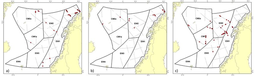
Leonard & Øien (2020)

Figure 7. Distribution of sightings recorded as sperm whales during the             Figure 6. Distribution of sightings recorded as killer whales during the
2014-2018 sighting surveys. The blue areas represent ice coverage.                  2014-2018 sighting surveys. The blue areas represent ice coverage.

Killer whales                                                                   Northern bottlenose whales
Killer whale observations were concentrated in the Norwegian                    Northern bottlenose whales were only detected in the
Sea (EW2, EW3) south of the Mohn Ridge and in the                               Iceland/Jan Mayen blocks and the neighbouring EW4 block
Icelandic/Jan Mayen survey blocks (CM1, CM3) (Figure 7). A                      (Figure 9). A half-normal model was fitted without covariates or
hazard-rate key function with group size as a covariate in the DS               truncation, producing an estimated p(0)=0.85 (CV=0.07) and
model, fitted to data truncated at 2000 m, provided the best                    eshw of 1122 m. The fitted DS and MR detection functions are
fitting detection function (Figure 8a). The probability of                      shown in Figure 10. The total corrected abundance of northern
detection on the transect line was estimated to be p(0)=0.86                    bottlenose whales was estimated to be 7,800 (CV=0.28, 95% CI:
(CV=0.06) with resulting eshw of 1031 m. Total corrected killer                 4,373–13,913). Detailed results by survey block are given in
whale abundance was estimated to be 15,056 (CV=0.29, 95% CI:                    Table 12.
8,423–26,914). Estimates by block are given in Table 9.

 Figure 8. Detection function curves for pooled detections (top) and the conditional detection probabilities of platform 1 (bottom) for (a) killer whales,
 (b) harbour porpoises, (c) Lagenorhynchus spp., and (d) northern bottlenose whales.

NAMMCO Scientific Publications, Volume 11                                                                                                                 8
Leonard & Øien (2020)
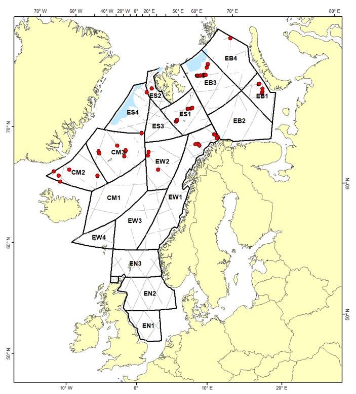
Figure 9. Distribution of northern bottlenose whales sighted during the Figure 11. Distribution of sightings recorded as harbour porpoises during
2014–2018 sighting surveys. The blue areas represent ice coverage. the 2014–2018 sighting surveys. The blue areas represent ice coverage.
Figure 10. Northern bottlenose whale. Photo credit: Jane Sproull
Thomson.
Harbour porpoises
Harbour porpoise sightings were concentrated in the North Sea
(EN1, EN2, EN3), the Barents Sea (EB1, EB2, EB3) (Figure 11).
BSS was included as a covariate in both the DS model and MR
models giving estimates of p(0)=0.47 (CV=0.13) and eshw of 260
m. The fitted DS detection function and MR conditional
Figure 12. Distribution of sightings recorded as Lagenorhynchus spp.
detection function are shown in Figure 8b. Total corrected during the 2014–2018 sighting surveys. The blue areas represent ice
harbour porpoise abundance was estimated to be 255,929 coverage.
(CV=0.20, 95% CI: 172,742–379,175) (Table 10).
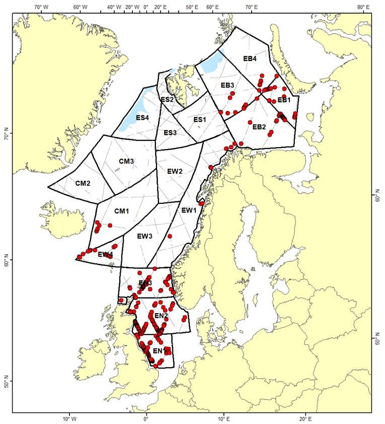
Lagenorhynchus spp. Other species
Lagenorhynchus spp. were encountered in most of the blocks Other species recorded, for which abundance has not been
within the study area, with the highest encounter rate in the estimated include blue whales, sei whales, bowhead whales,
Svalbard blocks (ES) and the Barents Sea (EB2) (Table 11; Figure and pilot whales. There were insufficient sightings for these
12). A hazard-rate model provided the best fit to the DS species; typically, a minimum of 20–30 observations are
detection function with BSS and group size as covariates and required to model a detection function using our methods
data truncated at 1200 m, resulting in an estimated p(0)=0.87 (Buckland et al., 2001). Blue whale sightings occurred in the
(CV=0.03) and eshw of 487 m. The fitted DS and MR detection blocks between Iceland and Svalbard, pilot whales were
functions are shown in Figure 7c. The total corrected abundance observed around the Faroe Islands, sei whales were spotted
of Lagenorhynchus spp. was estimated to be 192,767 (CV=0.25, west of Svalbard and south of Iceland, and bowhead whales
95% CI: 114,033–325,863). Detailed results by survey block are were observed along the ice edge in the northern Barents Sea
given in Table 11. (Figure 13).
NAMMCO Scientific Publications, Volume 11 9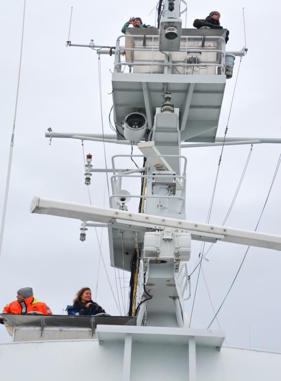
Leonard & Øien (2020)

To better understand the effect of unidentified large whale                  whales (17), blue whales (3), killer whales (17), Lagenorhynchus
sightings in the dataset, a detection function for these sightings           spp. (55), harbour porpoises (12) and northern bottlenose
was fit to the data, from which eshw was estimated to be 2,583               whales (2). Two sightings were recorded as ‘unidentified large
m (CV=0.10).                                                                 whales’. There were too few sightings of blue whales to
                                                                             estimate abundance using our methods and the small
                                                                             odontocetes were not estimated separately for the NASS
                                                                             extension.
                                                                             Estimates for small odontocetes observed in the EW blocks in
                                                                             2015 are reported as part of the regularly planned mosaic
                                                                             survey (Tables 9–12). The sightings from the modified CM
                                                                             blocks and EW blocks (Figure 1b) surveyed in 2015 were pooled
                                                                             to fit the detection function models.
                                                                             The fin whale was the most abundant large whale species in
                                                                             2015, with 80% of the sightings occurring in the northern most
                                                                             part of EW1, off the Finnmark coast of Norway (Figure 14a). A
                                                                             hazard-rate model provided the best fit to the DS detection
                                                                             function, with data truncated at 3500 m, resulting in an
                                                                             estimated p(0)=0.86 (CV=0.07) and eshw of 1508 m. The DS and
                                                                             MR detection functions are shown in Figure 15a. Total fin whale
                                                                             abundance in 2015 was estimated to be 3,729 (CV=0.44, 95% CI:
                                                                             1,531–9,081). Estimates by block are detailed in Table 13.
                                                                             As with fin whales, about 80% of humpback whale sightings
                                                                             occurred in the northern part of block EW1 (Figure 14b). Even
                                                                             with pooling across survey blocks, humpback whale sightings
                                                                             were insufficient to fit a detection function; thus, it was
                                                                             necessary to pool the data available from other years within the
                                                                             mosaic survey. Sightings recorded in 2014–2017 were used to
                                                                             fit a half-normal DS detection function. The sighting distance
Figure 13 Distribution of blue whales, sei whales, bowhead whales and        was truncated at 3000 m. The resulting model gave an estimate
pilot whales sighted during the 2014–2018 sighting surveys. The blue
                                                                             of p(0)=0.77 (CV=0.08) and eshw of 1260 m (Figure 15b). Total
areas represent ice coverage.
                                                                             corrected humpback whale abundance in 2015 was estimated
                                                                             to be 1,711 (CV=0.41, 95% CI: 604–3,631). Detailed results by
2015 and NASS extension estimates
                                                                             block are provided in Table 13.
A total effort of 7,857 km of transects was achieved in 2015,
                                                                             Figure 14c depicts the distribution of sperm whales observed in
covering a total area of 1,458,127 sq. km. The distribution of
                                                                             2015. The highest encounter rate occurred in the Norwegian
effort by Beaufort Sea State was 0.2% in BSS 0, 8% in BSS 1, 22%
                                                                             Sea, in EW3 and CM1a (Table 13). A half-normal DS model fitted
in BSS 2, 28% in BSS 3 and 44% in BSS 4. The survey achieved
                                                                             to data truncated at 3500 m gave an estimate of p(0)=0.70
good coverage of both the Small Management Area EW and the
                                                                             (CV=0.09) and eshw of 1685 m. The fitted detection functions
NASS extension CM Jan Mayen blocks. Survey block EW4 was
                                                                             are shown in Figure 15c. Total sperm whale abundance in 2015
not surveyed due to time constraints.
                                                                             was estimated to be 3,828 (CV=0.33, 95% CI: 1,994–7,595).
In 2015, there were 240 sightings of all whale species (Table 2).            Table 13 details the estimates by survey block.
These included fin whales (68), sperm whales (51), humpback

 Figure 14. 2015 NASS extension survey sightings: (a) fin whale sightings, (b) humpback whale sightings, and (c) sperm whale sightings.

NAMMCO Scientific Publications, Volume 11                                                                                                       10
Leonard & Øien (2020)
Figure 15. Detection function curves for pooled detections (top) and the conditional detection probabilities of platform 1 (bottom) for the NASS extension
survey in 2015 for (a) fin whales, (b) humpback whales, and (c) sperm whales.
Table 6. Estimated density and abundance of fin whales. The eshw (effective search half width (m)) was estimated for the entire study area. Encounter
rate, group size, density, abundance, and upper and lower confidence limits were estimated by block and corrected for perception bias, with the
estimated p(0).
Corrected 95% Confidence
Survey eshw Encounter Rate Group Size Density
Abundance Interval
Block
Estimate CV Estimate CV Estimate CV Estimate CV Lower Upper
CM1 0.002 1.078 1.00 0.000 0.001 1.080 151 1.080 9 2,440
CM2 0.020 0.328 1.33 0.121 0.006 0.328 1,029 0.328 461 2,298
CM3 0.010 0.565 1.00 0.000 0.003 0.555 836 0.555 223 3,132
EN1
EN2 0.000 0.932 1 0.000 0.000 0.934 25 0.934 4 147
EN3 0.009 0.506 1.30 0.220 0.002 0.511 378 0.511 117 1,214
ES1 0.021 0.469 1.46 0.141 0.006 0.474 1,025 0.474 357 2,944
ES2 0.031 0.418 1.09 0.018 0.011 0.453 563 0.453 223 1,425
ES3 0.025 0.553 1.10 0.058 0.008 0.560 891 0.560 250 3,173
2004.4 0.042
ES4 0.044 0.353 1.16 0.091 0.013 0.339 1,820 0.339 858 3,863
EW1 0.024 0.520 1.14 0.029 0.007 0.528 2,353 0.528 802 6,904
EW2 0.001 0.900 1.00 0.000 0.000 0.902 89 0.902 12 642
EW3 0.000 0.000 0.00 0.000 0.000 0.000 0 0.000 0 0
EW4 0.044 0.479 1.58 0.130 0.013 0.523 1,099 0.523 285 4,245
EB1 0.002 0.649 1.00 0.000 0.001 0.653 60 0.653 12 309
EB2 0.001 1.123 1.00 0.000 0.000 1.125 61 1.125 3 1,077
EB3 0.009 0.540 1.27 0.117 0.003 0.528 668 0.528 200 2,231
EB4 0.005 0.898 1.25 0.000 0.001 0.900 339 0.900 52 2,220
Total 0.003 0.173 11,387 0.173 8,072 16,063
NAMMCO Scientific Publications, Volume 11 11Leonard & Øien (2020)
Table 7. Estimated density and abundance of humpback whales. The eshw (effective search half width (m)) was estimated for the entire study
area. Encounter rate, group size, density, abundance, and upper and lower confidence limits were estimated by block and corrected for perception
bias, with the estimated p(0).
Corrected 95% Confidence
Survey eshw Encounter Rate Group Size Density
Abundance Interval
Block
Estimate CV Estimate CV Estimate CV Estimate CV Lower Upper
CM1
CM2 0.010 0.313 1.71 0.163 0.006 0.380 1,058 0.363 478 2,344
CM3 0.007 0.486 1.22 0.068 0.005 0.532 1,328 0.520 411 4,292
EN1
EN2
EN3
ES1 0.016 0.800 2.17 0.204 0.011 0.829 1,693 0.821 320 8,944
ES2 0.001 1.032 1.00 0.000 0.000 1.054 20 1.048 3 128
ES3
1086.9 0.173
ES4 0.002 1.042 1.00 0.000 0.001 1.064 143 1.058 20 1,033
EW1 0.006 0.533 1.33 0.184 0.004 0.575 1,201 0.564 392 3,679
EW2 0.002 0.500 1.00 0.000 0.001 0.545 296 0.533 89 987
EW3
EW4
EB1 0.018 0.781 1.42 0.155 0.012 0.811 1,134 0.803 173 7,442
EB2
EB3 0.026 0.836 1.175 0.037 0.017 0.864 3,684 0.856 624 21,747
EB4 0.001 0.898 1.00 0.000 0.001 0.923 151 0.916 23 982
Total 0.003 0.401 10,708 0.385 4,906 23,370
Table 8. Estimated density and abundance of sperm whales. The eshw (effective search half width (m)) was estimated for the entire study area.
Encounter rate, group size, density, abundance, and upper and lower confidence limits were estimated by block and corrected for perception
bias, with the estimated p(0).
Corrected 95% Confidence
Survey eshw Encounter Rate Group Size Density
Abundance Interval
Block
Estimate CV Estimate CV Estimate CV Estimate CV Lower Upper
CM1 0.017 0.356 1.08 0.076 0.007 0.393 1,944 0.395 709 5,329
CM2 0.005 0.965 1.00 0.000 0.002 0.980 329 0.980 41 2,612
CM3
EN1
EN2
EN3 0.001 1.073 1.00 0.000 0.000 1.086 40 1.087 5 340
ES1 0.006 0.631 1.00 0.000 0.002 0.653 405 0.654 103 1,600
ES2 0.002 0.739 1.00 0.000 0.001 0.758 38 0.758 9 160
ES3 0.007 0.380 1.00 0.000 0.003 0.416 329 0.417 132 817
1849 0.076
ES4 0.001 1.042 1.00 0.000 0.000 1.056 44 1.056 6 321
EW1 0.003 0.760 1.00 0.000 0.001 0.778 374 0.779 85 1,649
EW2 0.017 0.362 1.00 0.000 0.007 0.399 1,678 0.473 593 4,755
EW3 0.004 0.297 1.00 0.000 0.002 0.342 449 0.374 207 973
EW4 0.002 0.856 1.00 0.000 0.001 0.872 74 0.872 10 562
EB1
EB2
EB3
EB4
Total 0.002 0.253 5,704 0.263 3,374 9,643
NAMMCO Scientific Publications, Volume 11 12Leonard & Øien (2020)
Table 9. Estimated density and abundance of killer whales. The eshw (effective search half width (m)) was estimated for the entire study area. Encounter
rate, group size, density, abundance, and upper and lower confidence limits were estimated by block and corrected for perception bias, with the
estimated p(0).
Corrected 95% Confidence
Survey eshw Encounter Rate Group Size Density
Abundance Interval
Block
Estimate CV Estimate CV Estimate CV Estimate CV Lower Upper
CM1 0.030 0.409 3.76 0.215 0.016 0.485 4,861 0.485 1,519 15,555
CM2 0.004 0.969 5.00 0.000 0.002 1.004 404 1.004 51 3,181
CM3 0.014 0.533 3.10 0.169 0.009 0.616 2,595 0.616 655 10,278
EN1
EN2 0.001 1.045 3 0.000 0.001 1.063 198 1.063 29 1,354
EN3 0.002 0.909 3.00 0.000 0.001 0.930 228 0.930 34 1,514
ES1
ES2
ES3 0.019 0.491 2.43 0.071 0.015 0.542 1,768 0.542 547 5,712
1031.2 0.106
ES4
EW1 0.002 0.702 1.72 0.480 0.002 0.711 543 0.711 138 2,139
EW2 0.010 0.603 1.45 0.134 0.009 0.659 1,878 0.659 443 7,966
EW3 0.017 0.504 3.31 0.065 0.011 0.534 2,582 0.534 730 9,129
EW4
EB1
EB2
EB3
EB4
Total 0.004 0.293 15,056 0.293 8,423 26,914
Table 10. Estimated density and abundance of harbour porpoises. The eshw (effective search half width (m)) was estimated for the entire study area.
Encounter rate, group size, density, abundance, and upper and lower confidence limits were estimated by block and corrected for perception bias, with
the estimated p(0).
Corrected 95% Confidence
Survey eshw Encounter Rate Group Size Density
Abundance Interval
Block
Estimate CV Estimate CV Estimate CV Estimate CV Lower Upper
CM1 0.004 0.636 1.28 0.197 0.015 0.674 4,529 0.674 703 29,169
CM2
CM3
EN1 0.108 0.516 1.13 0.038 0.461 0.380 44,124 0.380 15,710 123,929
EN2 0.079 0.370 1.14 0.049 0.336 0.292 66,194 0.292 35,970 121,813
EN3 0.074 0.513 1.18 0.028 0.276 0.402 44,408 0.402 17,929 109,991
ES1
ES2
ES3
259.86 0.042
ES4
EW1 0.006 0.372 1.23 0.067 0.038 0.456 12,748 0.456 5,148 31,565
EW2
EW3
EW4 0.024 0.331 1.28 0.037 0.129 0.325 10,943 0.325 5,237 22,866
EB1 0.035 0.594 1.30 0.096 0.112 0.457 11,947 0.457 3,719 38,376
EB2 0.035 0.784 1.15 0.038 0.130 0.638 36,369 0.638 6,083 217,446
EB3 0.018 0.679 1.33 0.070 0.067 0.560 15,592 0.560 4,478 54,288
EB4 0.015 0.687 1.35 0.141 0.039 0.633 9,075 0.633 2,234 36,863
Total 0.075 0.197 255,929 0.197 172 742 379,175
NAMMCO Scientific Publications, Volume 11 13Leonard & Øien (2020)
Table 11. Estimated density and abundance of Lagenorhynchus spp. The eshw (effective search half width (m)) was estimated for the entire study area.
Encounter rate, group size, density, abundance, and upper and lower confidence limits were estimated by block and corrected for perception bias,
with the estimated p(0).
Corrected 95% Confidence
Survey eshw Encounter Rate Group Size Density
Abundance Interval
Block
Estimate CV Estimate CV Estimate CV Estimate CV Lower Upper
CM1 0.001 1.078 2.00 0.000 0.001 1.102 350 1.102 23 5,174
CM2 0.003 1.027 4.00 0.000 0.003 1.047 451 1.046 55 4,152
CM3 0.001 0.949 2.00 0.000 0.001 0.976 379 0.976 49 2,864
EN1 0.014 0.513 3.57 0.138 0.015 0.539 1,510 0.582 293 7,069
EN2 0.031 0.565 2.68 0.143 0.032 0.569 6,371 0.569 1,944 20,511
EN3 0.037 0.635 2.63 0.164 0.038 0.588 6,403 0.588 1,626 23,236
ES1 0.367 0.618 4.26 0.044 0.311 0.575 55,932 0.575 15,719 194,939
ES2 0.173 0.424 3.44 0.107 0.165 0.436 8,884 0.436 3,634 21,947
ES3 0.155 0.606 4.01 0.077 0.144 0.583 16,725 0.583 4,662 64,979
487.4 0.037
ES4
EW1 0.050 0.662 3.16 0.109 0.051 0.648 17,713 0.647 4,761 62,522
EW2
EW3 0.007 1.026 3.02 0.033 0.007 1.028 1,694 1.027 158 17,428
EW4 0.008 0.856 7.00 0.000 0.007 0.859 589 0.859 80 4,851
EB1 0.093 0.562 4.42 0.166 0.073 0.557 7,059 0.545 1,719 28,117
EB2 0.171 0.535 3.02 0.071 0.177 0.538 52,629 0.540 10,250 246,260
EB3 0.054 0.255 2.53 0.090 0.055 0.273 13,400 0.286 6,817 24,585
EB4 0.016 0.709 4.74 0.122 0.013 0.743 2,684 0.743 601 14,714
Total 0.055 0.242 192,768 0.248 114,033 325,863
Table 12. Estimated density and abundance of northern bottlenose whales. The eshw (effective search half width (m)) was estimated for the entire
study area. Encounter rate, group size, density, abundance, and upper and lower confidence limits were estimated by block and corrected for
perception bias, with the estimated p(0).
Corrected 95%
Survey eshw Encounter Rate Group Size Density
Abundance Confidence Interval
Block
Estimate CV Estimate CV Estimate CV Estimate CV Lower Upper
CM1 0.013 0.636 2.62 0.116 0.007 0.652 2,027 0.652 336 12,246
CM2 0.017 0.595 2.63 0.243 0.009 0.433 1,601 0.433 587 4,365
CM3 0.023 0.314 2.13 0.184 0.012 0.342 3,553 0.342 1,628 7,751
EN1
EN2
EN3
ES1
ES2
ES3
1121.95 0.088
ES4
EW1
EW2
EW3
EW4 0.014 1.080 3.00 0.263 0.007 0.741 617 0.741 104 3,678
EB1
EB2
EB3
EB4
Total 0.002 0.280 7,800 0.280 4,373 13,913
NAMMCO Scientific Publications, Volume 11 14Leonard & Øien (2020)
Table 13. Estimated density and abundance of large whale species from the NASS extension survey conducted in 2015. The eshw (effective search
half width (m)) and p(0) were estimated for the entire study area. Encounter rate, group size, density, abundance and upper and lower confidence
limits were estimated by block and corrected for perception bias, with the estimated p(0)).
Corrected 95% Confidence
Survey eshw p(0) Encounter Rate Group Size Density
Sp. Abundance Interval
Block
Estimate CV Estimate CV Estimate CV Estimate CV Estimate CV Estimate CV Lower Upper
CM1a 0.002 0.933 1.00 0.000 0.001 0.940 101 0.940 4 2,830
CM3a 0.005 0.718 1.29 0.025 0.002 0.727 579 0.727 111 3,016
EW1 1507.9 7.47 0.861 0.085 0.019 0.508 1.14 0.030 0.009 0.534 2,935 0.534 1,005 8,573
Fin
EW2 0.001 0.914 1.00 0.000 0.001 0.921 114 0.921 15 839
EW3
Total 0.002 0.442 3,729 0.442 1,531 9,081
CM1a
CM3a 0.004 0.418 1.18 0.065 0.002 0.445 555 0.445 223 1,380
Humpback
EW1 1260.1 11.26 0.771 0.104 0.006 0.534 1.33 0.184 0.003 0.555 933 0.555 307 2,835
EW2 0.002 0.481 1.00 0.000 0.001 0.505 224 0.505 70 715
EW3
Total 0.000 0.410 1,712 0.410 604 3,631
CM1a 0.021 0.470 1.00 0.000 0.009 0.523 1,465 0.523 313 6,870
CM3a 0.002 0.729 1.00 0.000 0.001 0.764 215 0.764 41 1,127
Sperm
EW1 1684.7 10.84 0.692 0.203 0.003 0.761 1.00 0.000 0.001 0.795 396 0.795 90 1,755
EW2 0.016 0.328 1.00 0.000 0.007 0.401 1,460 0.401 624 3,416
EW3 0.004 0.302 1.00 0.000 0.002 0.380 355 0.380 156 808
Total 0.002 0.328 3,891 0.328 1,994 7,595
sighted at shorter distances, they too show higher uncertainty
DISCUSSION AND CONCLUSIONS
in duplicate judgement, likely due to their group behaviour.
Being gregarious species, dolphins join, split, and re-join groups
Bias and estimation issues
continuously, which makes it difficult to match duplicates of
Survey coverage multiple small groups over a short range. We also expect there
to be higher risk of error in observer measurements of group
While survey coverage was acceptable in most areas, ice
size, distance, and angles when observing groups of animals
coverage hampered efforts in the northernmost regions of the
(Buckland et al., 2001). The exclusion of less certain duplicate
study area, reducing the survey area coverage by 2.6%. This is
identifications may lead to an underestimation of p(0) and
similar to past surveys (Øien, 2009; Leonard & Øien, 2020) and
positively biased estimates. For this reason, we accepted the
should not have a large effect on overall abundance, as these
D+P duplicates to estimate abundance.
species are not expected to aggregate in ice covered areas.
Species identification
Duplicate identification uncertainty
Failure to identify some sightings to species likely resulted from
In this analysis, duplicate judgements were given a subjective
the focus on minke whales and the fact that whales were
confidence rating, which had not been done for previous
observed in passing mode. Identification of non-target species
surveys. By comparing 3 estimates of p(0), first using only
was likely further compromised when tracking procedures for
definite duplicates (D), then including probable duplicates
minke whales were underway (Skaug et al., 2004). Comparing
(D+P), then remote duplicates (D+P+R), the effect of duplicate
the eshw for ‘unidentified large whale’ sightings (2583 m) to the
uncertainty on the abundance estimates could be investigated.
eshw for fin, humpback and sperm whales (2004 m, 1087 m and
Generally, we expect that duplicate uncertainty is higher in our
1849 m, respectively), we find that the sightings of ‘unidentified
surveys than some other surveys, for example SCANS surveys
large whales’ were made at greater distances than identified
(Hammond et al., 2002; 2013), because only initial sightings are
large whales. Given that detections that occur far from the
recorded for non-target species. We found no significant
transect line have a reduced effect on the scale of the detection
difference (p>0.05) between the estimates of p(0) for D+P+R
function, we expect their effect on estimates of density to be
duplicates and for the D+P duplicates used in this analysis,
fairly small.
however we did find a significant difference (pLeonard & Øien (2020)
result in an underestimation of the abundance; however, given variance we observe. For example, in block EW1 the density of
the challenges our methods pose for duplicate judgement humpback whales is concentrated in the northern part of the
(discussed above under section Duplicate identification block, suggesting our stratification is not ideal for the species
uncertainty) we expect that an underestimation of p(0) and (Figure 5).
positively biased estimates are more likely. In future surveys,
A potential alternative to design-based estimates is to use a
providing a confidence rating for each identification, as was
model-based approach, which would allow for fitting models as
done for duplicate judgements, would allow for a sensitivity
a function of spatially referenced environmental variables. This
analysis of the effect of the uncertainty in species identification.
would account for some of the spatial variation in the
Additionally, it is also possible to apportion the unidentified
distribution of non-target species.
large whales to species based on their relative abundance
(Rogan et al., 2017). This was not done here, however, as it Harbour porpoise estimates and Beaufort Sea State
could introduce further bias if identification uncertainty differs
between species or regions. Survey effort used to estimate harbour porpoise abundance is
typically restricted to BSS of 2 or less because of their reduced
Distance estimation detectability at higher sea states (Barlow, 1988; Hammond et
al., 2002; 2013). We opted to use all data up to BSS of 4 because
Bias in distance estimation is perhaps one of the greatest
encounter rates were reasonably high at higher sea states in our
sources of error in line transect surveys, particularly when
survey, and because including all survey effort resulted in lower
distance measurements rely on naked-eye measurements
variance in estimated abundance than when restricting BSS to 2
(Leaper, Burt, Gillespie, & Macleod, 2010). Error in distance
or less. The inclusion of BSS and other covariates appears to
measurements can affect both the successful identification of
have been effective for modelling the lower detectability at
duplicates and the overall shape of the detection function
higher sea states in our data. This conclusion was reviewed and
(Buckland et al., 2001). This is complicated by the fact that the
supported by the NAMMCO Abundance Estimates Working
bias may be non-linear, where large distances are
Group (NAMMCO, 2019). Thus, we conclude that the model
underestimated and short distances, overestimated (Leaper et
constructed utilizing all harbour porpoise sightings (BSS 0–4) is
al., 2010). Our survey, which has been using consistent methods
appropriate for estimating harbour porpoise abundance for this
since 1995 (Øien, 1995), attempts to mitigate this type of error
survey.
by maintaining experienced observers and providing regular
training. In future surveys, the effect of this type of error could Comparison to past surveys
be evaluated by validating some proportion of the
measurements through the use of precise distance-measuring Fin whales
devices such as cameras, reticle binoculars, or drones. The distribution of fin whales in our surveys was similar to what
Distributional shifts was found in past surveys where fin whales were most
abundant in the Icelandic blocks and Svalbard blocks, ranging
Shifts in a species’ distribution between survey years and from the Finnmark coast to Bear Island, and northwards to the
between survey blocks increases the variance in the estimates westernmost point of Spitsbergen (ES1, ES2). Our survey
for a mosaic survey conducted over several years to an estimated 11,387 (CV=0.17, 95% CI: 8,072–16,063) fin whales
unknown degree. Additional variance has been accounted for in overall, which is consistent with the past two surveys, which
minke whale estimates (Bøthun et al., 2009; Solvang et al., found corrected estimates of ~10,000 fin whales (Leonard &
2015); however, this has not been possible for other species due Øien, 2020).
to the lack of necessary information regarding population
growth, movement, residency, etc. Humpback whales
Since the mosaic survey program began, steps have been taken Our humpback whale abundance estimate of 10,708 (CV=0.39,
to reduce the potential for additional variance by surveying 95% CI: 4,906–23,370) falls within the range of the previous two
each SMA within a single year (Skaug et al., 2004). This was surveys of 12,411 (CV=0.30, 95% CI: 6,847–22,497) in 2008–
successfully achieved in this survey cycle with the exception of 2013 and 9,749 (CV=0.34, 95% CI: 4,947–19,210) in 2002–2007
block EW4, which was surveyed in 2018 rather than 2015 due (Leonard & Øien, 2020). This suggests that the rather dramatic
to time constrains. These measures are intended to reduce the increase in humpback whale occurrence in Norwegian waters
variance for minke whales for which the SMAs are defined. since our earlier surveys in 1995 and 1996–2001 (Øien, 2009)
However, given that the SMAs are large geographic regions with has now subsided and the population has stabilised over the last
unique physical and biological distinctions, surveying them 3 survey periods.
completely within a single year may also reduce the variance for The increase in abundance we have observed, beginning in
regional species such as dolphins and other small odontocetes. 2002–2007, appears to have occurred largely in the Bear Island
Encounter rate variance shelf area and the northern Barents Sea (Øien, 2009). We
estimated 1,693 (CV=0.82, 95% CI: 320–8,944) for the Bear
Variance in estimated encounter rate was typically high for all Island area (block ES1), while the past two surveys estimated
non-target species (Tables 6–13). For design-based estimates, 4,040 (CV=0.52 95% CI: 1,304–12,515 in block BJ) in 2002–2007
encounter rate variance can be minimised by creating survey and 3,963 (CV=0.45, 95% CI: 1,197–13,117) in 2008–2013
blocks, within which the density of a species is homogeneously (Leonard & Øien, 2020). Older surveys estimated an
distributed, and the transects are placed perpendicular to any uncorrected abundance of 144 (CV=0.61, 95% CI: 34–601) in
density gradients (Buckland et al., 2001). This is generally not 1996–2001 and 656 (CV=0.31, 95% CI: 344–1,253) in 1995. The
possible for multiple species within a survey; thus, our minke- summed estimates for the Barents Sea (EB blocks) in the 2014–
whale-tailored design likely contributes to the encounter-rate 2018 survey period was 4,968. Estimates for the same area in
NAMMCO Scientific Publications, Volume 11 16Leonard & Øien (2020)
2002–2007 and 2008–2013 were 1,832 and 4,292, respectively A much lower estimate of harbour porpoises was found for the
(Leonard & Øien, 2020), while the older, uncorrected estimates North Sea in our 2008–2013 survey (38,351 CV=0.58, 95% CI:
in comparable blocks (BAE, KO, GA) found 118 humpback 13,158–111,777), but this was considered to be an anomaly
whales in 1995 and 54 humpback whales in 1996–2001 (Øien, (Leonard & Øien, 2020).
2009). Given that the humpback whales we observe in
Lagenorhynchus spp.
Norwegian waters are part of a much larger population (Smith,
2010; Smith et al., 1999), we cannot distinguish between what Our total abundance estimate of 192,767 (CV=0.25, 95% CI:
might be population growth versus immigration, without an 114,033–325,863) Lagenorhynchus dolphins of is comparable to
effort to identify and track humpback whales between our past survey periods. The 2008–2013 survey estimated an
study area and other feeding grounds. Nevertheless, the abundance of 163,688 (CV=0.18, 95% CI: 112,673–237,800) and
Barents Sea ecosystem appears to have become an attractive the 2002–2007 survey estimated 213,070 (uncorrected,
area for North Atlantic humpback whales in recent decades and CV=0.18 95% CI: 144,720–313,690) from a single platform
this is likely due to the dramatic shifts in Atlantic herring and (Leonard & Øien, 2020).
capelin abundances that coincide with our surveys (Gjøsæter,
Bogstad, & Tjelmeland, 2009). White-beaked dolphins have made up 90% of sightings for
Lagenorhynchus spp. in our study area (Øien, 1996), and this is
Sperm whales consistent with what we found, where 94% of Lagenorhynchus
spp. identified to species level were white-beaked dolphins. Our
Sperm whale distribution has been consistent among survey
data also suggest that the observations in the northern part of
periods and is generally associated with the deep water of the
the study region are almost exclusively white-beaked dolphins
Norwegian Sea basin. The 2014–2018 survey estimated 5,704
while white-sided dolphins tend to be observed in the south
(CV=0.26, 95% CI: 3,374–9,643) sperm whales, within the range
(Figure 12). Observer effort to identify dolphin species has
of the two prior survey estimates: 8,134 (CV=0.18, 95% CI:
improved from earlier surveys. However, due to the focus on
5,695–11,617) in 2002–2007 and 3,962 (CV=0.29, 95% CI:
minke whales and that fact that the northern regions tend to be
2,218–7,079) in 2008–2013. It is comparable to older survey
‘busier’ with sightings, this improvement may not be even
estimates (6,375 (CV=0.22; 95% CI: 4,163–9,762) in 1996–2001
across the study region, with a greater potential to identify
and 4,319 (CV=0.20 95% CI: 2,903–6,424) in 1995), although
dolphins to species in the ‘quieter’ southern survey regions. For
these were not corrected for perception bias (Øien, 2009). Our
this reason, we estimate Lagenorhynchus spp. to genus only.
estimates do not account for availability bias, which could be an
issue for sperm whales as they spend long periods of time Northern bottlenose whales
underwater on deep dives (Drouot, Gannier, & Goold, 2004;
Watkins, Moore, Tyack, 1985). This likely results in an The abundance of northern bottlenose whales was not
underestimate for this species. estimated in our earlier surveys due to there being too few
observations. In the past two surveys (Leonard & Øien, 2020),
Killer whales there were 12 sightings (2002–2007), and 10 sightings (2008–
2013) with distributions consistent with what we have observed
The current estimate for killer whales (15,056; CV=0.29 95% CI:
in the current survey (Figure 9). The region between Svalbard
8,423–26,914) falls between the previous two survey estimates
and Jan Mayen, where most of our sightings occurred, was an
of 9,563 (CV=0.36, 95% CI: 4,713–19,403) in 2008–2013 and
area of intense whaling of northern bottlenose whales up to
18,821 (CV=0.24, 95% CI: 11,525–30,735) in 2002–2007.
1973 (Reeves, Mitchell, & Whitehead, 1993) and the population
Variation among repeated survey estimates has been noted for
likely remains depleted (Benjaminsen & Christensen, 1979).
surveys of neighbouring regions (Foote et al., 2007), suggesting
While there are no directly comparable recent estimates for this
that killer whales may have a highly variable summer
region, one of the Faroese blocks (block FC) from the 2015
distribution. Our estimates of killer whale abundance may also
Icelandic and Faroese NASS survey covered an area of partial
be susceptible to additional variance due to distributional shifts
overlap with the CM1 and EW4 blocks in our 2016 survey and
from one year to the next, given that they are local species
generated an estimate of 11,384 (CV=0.94, 95% CI: 1,492–
thought to be strongly associated with dynamic distributions in
86,861) northern bottlenose whales (Pike et al., 2019,
prey (Nøttestad, 2015). The population size of the killer whales
supplementary file 8). Combining the total Icelandic-Faroese
in the entire North Atlantic is not known, however, a report on
estimate of 19,975 (CV=0.06, 95% CI: 5,562–71,737) (Pike et al.,
the status of killer whales in the North Atlantic was published
2019) with the part of our estimate of 7,800 (CV=0.28, 95% CI:
recently and summarizes all of the estimates available (Jourdain
4,373–13,913) that does not overlap with the FC block, provides
et al., 2019). Our survey estimates can contribute to filling some
a recent estimate for the whole Northeast Atlantic. Similar to
of the gaps in the population status of North Atlantic killer
sperm whales, northern bottlenose whales are deep divers that
whales.
spend long periods underwater (Hooker & Baird, 1999), which
Harbour porpoises likely results in a negative bias in our estimates.
Our 2014–2018 estimate of harbour porpoise abundance
(255,929 CV=0.20, 95% CI: 172,742–379,175) was similar to the ADHERENCE TO ANIMAL WELFARE PROTOCOLS
2002–2007 estimate of 189,604 (CV=0.19, 95% CI: 129,437–
277,738) (Leonard & Øien, 2020). Our estimate is also The research presented in this article has been done in
comparable to SCANS surveys for the North Sea, which accordance with the institutional and national animal welfare
estimated 355,408 (CV=0.22) in 2005 and 245,373 (CV=0.18) in laws and protocols applicable in the jurisdictions in which the
2016 (Hammond et al., 2013, 2017). work was conducted.
NAMMCO Scientific Publications, Volume 11 17Leonard & Øien (2020)
ACKNOWLEDGEMENTS Hooker, S. K., & Baird, R. W. (1999). Deep-diving behaviour of the
northern bottlenose whale, Hyperoodon ampullatus (Cetacea:
Ziphiidae). Proceedings of the Royal Society B: Biological Sciences,
The project was made possible through funding provided by 266(1420), 671-676. https://doi.org/10.1098/rspb.1999.0688
IMR with analysis support from NAMMCO. We are grateful to International Whaling Commission (IWC). (1994). Report of the
the Scientific Committee of NAMMCO and the NAMMCO Scientific Committee. Annex K. Area definitions for RMP
Secretariat for their contributions to reviewing our analyses and implementations. Report of the International Whaling
coordinating this publication. We thank the crew of all Commission, 44, 175-176.
participating vessels and the Coastguard for making vessels International Whaling Commission (IWC). (2004). Report of the
available to us. We’d also like to thank our excellent observers Scientific Committee. Annex D, Appendix 14. Report of the
working group on North Atlantic minke whales RMP
and team leaders for dedication and hard work. Last but not
Implementation Review. Journal of Cetacean Resource
least, we would like to acknowledge Kjell Arne Fagerheim and Management, 6(Supplement), 171-183.
Siri Hartvedt for their painstaking efforts in preparing and Jourdain, E., Ugarte, F., Víkingsson, G. A., Samarra, F. I., Ferguson, S. H.,
validating the data. Tusen takk fra oss! Lawson, J., ... & Desportes, G. (2019). North Atlantic killer whale
Orcinus orca populations: a review of current knowledge and
REFERENCES threats to conservation. Mammal Review, 49(4), 384-400.
https://doi.org/10.1111/mam.12168
Laake, J. L., & Borchers, D. L. (2004). Methods for incomplete detection
Barlow, J. (1988). Harbour porpoise, Phocoena phocoena, abundance
at distance zero. In S. T. Buckland, D. R. Anderson, K. P. Burnham,
estimation for California, Oregon and Washington. Ship surveys.
J. L. Laake, D. L. Borchers & L. Thomas. (eds.), Advanced Distance
Fishery Bulletin (US), 86, 417– 432.
Sampling, 108-189. London: Oxford University Press.
Benjaminsen, T., & Christensen, I. (1979). The natural history of the
Leaper, R., Burt, L., Gillespie, D., & Macleod, K. (2010). Comparisons of
bottlenose whale, Hyperoodon ampullatus (Forster). In H. E. Winn
measured and estimated distances and angles from sightings
& B. L. Olla (eds.), Behavior of Marine Animals: Current
surveys. Journal of Cetacean Research and Management, 11,
Perspectives in Research, 143-164. Boston, MA: Springer US.
229–237.
https://doi.org/10.1007/978-1-4684-2985-5_5
Leonard, D. M., & Øien, N. (2020). Estimated abundances of cetacean
Buckland, S. T., Anderson, D. R., Burnham, K. P., Laake, J. L., Borchers,
species in the Northeast Atlantic from shipboard surveys
D. L., & Thomas, L. (2001). Introduction to Distance Sampling.
conducted between 2002-2013. NAMMCO Scientific Publications,
London: Oxford University Press. https://doi.org/10.1111/j.1365-
11. https://doi.org/ 10.7557/3.4695
2664.2009.01737.x
North Atlantic Marine Mammal Commission (NAMMCO). (2019).
Bøthun, G., Skaug, H. J., & Øien, N. (2009). Abundance of minke whales
Report of the Abundance Estimates Working Group, October
in the Northeast Atlantic based on survey data collected over the
2019, Tromsø, Norway. Retrieved from
period 2002-2007. Unpublished manuscript (Document
https://nammco.no/topics/abundance_estimates_reports/
SC/61/RMP2 for the IWC Scientific Committee).
Nøttestad, L., Krafft, B. A., Anthonypillai, V., Bernasconi, M., Langård, L.,
Christensen, I., Haug, T., & Øien, N. (1992). Seasonal distribution,
Mørk, H. L., & Fernö, A. (2015). Recent changes in distribution and
exploitation and present abundance of stocks of large baleen
relative abundance of cetaceans in the Norwegian Sea and their
whales (Mysticeti) and sperm whales (Physeter macrocephalus) in
relationship with potential prey. Frontiers in Ecology and
Norwegian and adjacent waters. ICES Journal of Marine Science,
Evolution, 2, 83. https://doi.org/10.3389/fevo.2014.00083
49(3), 341-355. https://doi.org/10.1093/icesjms/49.3.341
Pike, D. G., Gunnlaugsson, T., Mikkelsen, B., Halldórsson, S. D., &
Drouot, V., Gannier, A., & Goold, J. C. (2004). Diving and feeding
Víkingsson, G. A. (2019). Estimates of the abundance of cetaceans
behaviour of sperm whales (Physeter macrocephalus) in the
in the central North Atlantic based on the NASS Icelandic and
northwestern Mediterranean Sea. Aquatic mammals, 30(3), 419-
Faroese shipboard surveys conducted in 2015. NAMMCO
426. https://doi.org/10.1578/AM.30.3.2004.419
Scientific Publications, 11. https://doi.org/10.7557/3.4941
Fewster, R. M., Buckland, S. T., Burnham, K. P., Borchers, D. L., Jupp, P.
Schweder, T., Skaug, H. J., Dimakos, X. K., Langaas, M., & Øien, N. (1997).
E., Laake, J. L., & Thomas, L. (2009). Estimating the Encounter Rate
Abundance of northeastern Atlantic minke whales, estimates for
Variance in Distance Sampling. Biometrics, 65, 225-236.
1989 and 1995. Report of the International Whaling Commission,
https://doi.org/10.1111/j.1541-0420.2008.01018.x
47, 453-483.
Foote, A. D., Vıkingsson, G., Øien, N., Bloch, D., Davis, C. G., Dunn, T. E.,
Skaug, H.J., Øien, N., Schweder, T., & Bøthun, G. (2004). Abundance of
... & Thompson, P. M. (2007). Distribution and abundance of killer
minke whales (Balaenoptera acutorostrata) in the Northeastern
whales in the North East Atlantic. IWC/SC/59/SM, 5(10).
Atlantic. Canadian Journal of Fisheries and Aquatic Science, 61(6),
Gjøsæter, H., Bogstad, B., & Tjelmeland, S. (2009). Ecosystem effects of
870-886. https://doi.org/10.1139/f04-020
the three capelin stock collapses in the Barents Sea. Marine
Solvang, H. K., Skaug, H. J., & Øien, N. I. (2015). Abundance estimates of
Biology Research, 5, 40-53.
common minke whales in the Northeast Atlantic based on survey
https://doi.org/10.1080/17451000802454866
data collected over the period 2008-2013. Unpublished
Hammond, P. S., Berggren, P., Benke, H., Borchers, D. L., Collet, A.,
manuscript (Document SC/66a/RMP8 for the IWC Scientific
Heide-Jørgensen, M. P., … & Øien, N. (2002). Abundance of
Committee).
harbour porpoise and other cetaceans in the North Sea and
Reeves, R. R., Mitchell, E., & Whitehead, H. (1993). Status of the
adjacent waters. Journal of Applied Ecology, 39, 361–376.
northern bottlenose whale, Hyperoodon ampullatus in Canada.
https://doi.org/10.1046/j.1365-2664.2002.00713.x
Committee on the Status of Endangered Wildlife in Canada,
Hammond, P. S., Lacey, C., Gilles, A., Viquerat, S., Börjesson, P., Herr, H.,
Ottawa, 16pp.
… & Øien, N. (2017). Estimates of cetacean abundance in
Rogan, E., Cañadas, A., Macleod, K., Santos, M. B., Mikkelsen, B.,
European Atlantic waters in summer 2016 from the SCANS-III
Uriarte, A., ... & Hammond, P. S. (2017). Distribution, abundance
aerial and shipboard surveys. SCANS-III project report 1, 39pp.
and habitat use of deep diving cetaceans in the North-East
Retrieved from
Atlantic. Deep Sea Research Part II: Topical Studies in
https://synergy.st-andrews.ac.uk/scans3/files/2017/05/SCANS-
Oceanography, 141, 8-19.
III-design-based-estimates-2017-05-12-final-revised.pdf
https://doi.org/10.1016/j.dsr2.2017.03.015
Hammond, P.S., Macleod, K., Berggren, P., Borchers, D.L., Burt, L.,
Smith, T. D., Allen, J., Clapham, P. J., Hammond, P. S., Katona, S., Larsen,
Cañadas, A., … & Gordon, J. (2013). Cetacean abundance and
F., ... & Øien, N. (1999). An ocean basin wide mark recapture study
distribution in European Atlantic shelf waters to inform
of the north Atlantic humpback whale (Megaptera novaeangliae).
conservation and management. Biological Conservation, 164,
Marine Mammal Science, 15(1), 1-32.
107-122. https://doi.org/10.1016/j.biocon.2013.04.010
NAMMCO Scientific Publications, Volume 11 18You can also read