Evaluation of Daily Precipitation from the ERA5 Global Reanalysis against GHCN Observations in the Northeastern United States - MDPI
←
→
Page content transcription
If your browser does not render page correctly, please read the page content below
climate
Article
Evaluation of Daily Precipitation from the ERA5
Global Reanalysis against GHCN Observations in the
Northeastern United States
Caitlin C. Crossett 1,2, *, Alan K. Betts 1,3 , Lesley-Ann L. Dupigny-Giroux 1,4 and
Arne Bomblies 1,2
 1    Vermont EPSCoR, University of Vermont, Burlington, VT 05405, USA; akbetts@aol.com (A.K.B.);
      ldupigny@uvm.edu (L.-A.L.D.-G.); abomblie@uvm.edu (A.B.)
 2    Department of Civil and Environmental Engineering, University of Vermont, Burlington, VT 05405, USA
 3    Atmospheric Research, Pittsford, VT 05763, USA
 4    Department of Geography, University of Vermont, Burlington, VT 05405, USA
 *    Correspondence: ccrosset@uvm.edu

 Received: 27 November 2020; Accepted: 14 December 2020; Published: 15 December 2020

 Abstract: Precipitation is a primary input for hydrologic, agricultural, and engineering models,
 so making accurate estimates of it across the landscape is critically important. While the
 distribution of in-situ measurements of precipitation can lead to challenges in spatial interpolation,
 gridded precipitation information is designed to produce a full coverage product. In this study,
 we compare daily precipitation accumulations from the ERA5 Global Reanalysis (hereafter ERA5)
 and the US Global Historical Climate Network (hereafter GHCN) across the northeastern United
 States. We find that both the distance from the Atlantic Coast and elevation difference between ERA5
 estimates and GHCN observations affect precipitation relationships between the two datasets.
 ERA5 has less precipitation along the coast than GHCN observations but more precipitation
 inland. Elevation differences between ERA5 and GHCN observations are positively correlated
 with precipitation differences. Isolated GHCN stations on mountain peaks, with elevations well
 above the ERA5 model grid elevation, have much higher precipitation. Summer months (June, July,
 and August) have slightly less precipitation in ERA5 than GHCN observations, perhaps due to the
 ERA5 convective parameterization scheme. The heavy precipitation accumulation above the 90th,
 95th, and 99th percentile thresholds are very similar for ERA5 and the GHCN. We find that daily
 precipitation in the ERA5 dataset is comparable to GHCN observations in the northeastern United
 States and its gridded spatial continuity has advantages over in-situ point precipitation measurements
 for regional modeling applications.

 Keywords: precipitation; climate; ERA5; GHCN; northeastern US; hydrology

1. Introduction
      Accurate representations of precipitation across a landscape are important in the design of various
engineering systems, as well as in the modeling of meteorological, hydrologic, and agricultural
systems. This is especially true for the northeastern United States (hereafter Northeast). The Northeast
is classified as a humid continental climate [1] and is characterized by complex terrain, a coast
that borders the Atlantic Ocean, and a large number of metropolitan areas. Attempts to model
hydrologic systems or draw conclusions from these models over large areas of complex topography
using only in-situ precipitation gauges are subject to errors from missing data, large interpolation
distances, a non-uniform distribution of gauges, and difficulty in the generalizability of results.

Climate 2020, 8, 148; doi:10.3390/cli8120148                                   www.mdpi.com/journal/climate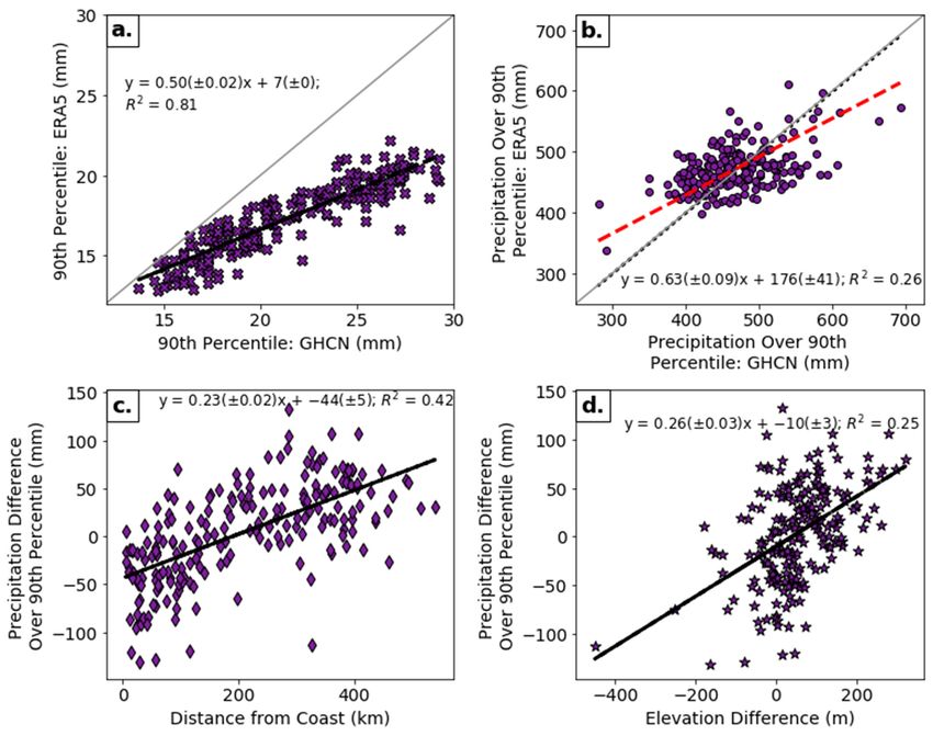
Climate 2020, 8, 148 2 of 14
Therefore, researchers have looked to using gridded precipitation information [2] such as the Daymet
Dataset (spatial interpolation) [3], Meteorological Forcing Dataset (observation-based land surface
forcings, derived surface fluxes and state variables) [4,5], the Parameter-elevation Regressions on
Independent Slopes Model (PRISM; gridded precipitation estimates adjusted by physiographic
factors) [6] and the ERA5 Global Reanalysis (hereafter ERA5; [7]) to address the challenges posed by
in-situ observations. ERA5 is the most recent global climate reanalysis from the European Centre for
Medium-Range Weather Forecasts (ECMWF) and represents an improvement over its predecessor
ERA-Interim [8] in both spatial and temporal resolutions, and 2 m temperature accuracy [9]. ERA5 not
only includes a robust physical and dynamic model of the atmosphere but also assimilates millions
of observations into its reanalysis forecasts, making it suitable for reconstructing the climate past.
Information from ERA5 allows the user to analyze continuous processes in a framework with fully
coupled land, atmosphere, and ocean dynamics. With its complex topography, proximity to the
Atlantic Ocean, and large population centers, the Northeast is a prime location to evaluate the utility of
ERA5 for hydrologic and other applications.
Existing literature on the performance of the ERA5 dataset over the continental United
States for hydrologic and precipitation studies has found that, while ERA5 performs better in
hydrologic simulations than its predecessor ERA-Interim for all regions, it does not perform as
well as actual observations for the eastern United States, perhaps due to the higher station density
there [10]. For example, Beck et al. [11] compared 15 uncorrected precipitation datasets across
the Northeast and found that ERA5 performed the best overall (with the highest Kling-Gupta
Efficiency score [12,13]), especially in complex terrain when compared to the IMERGHHE V05 satellite
precipitation product [14,15]. However, the opposite is true in locations dominated by small-scale
convectively driven precipitation when compared to IMERGHHE V05 [11]. There are challenges in
comparing an in-situ measurement of precipitation to a distributed precipitation product, such as a
gridded dataset. This is primarily due to the fact that an in-situ measurement is only representative of
the immediate surroundings in which it is located, whereas a distributed measurement of precipitation
smooths information over a larger region. The scales on which in-situ and distributed measurements
of precipitation can be applied need to be carefully considered.
In addition to using ERA5 for hydrologic modeling purposes [10] it is useful to assess how well
ERA5 represents heavy precipitation events across the Northeast. Heavy precipitation events can be
defined in a number of ways and generally fall in the right tail of a precipitation distribution (statistically
the 75th to 99th percentile). Some studies, e.g., Huang et al. [16], Marquardt Collow et al. [17],
Frei et al. [18], Guilbert et al. [19], and Hayhoe et al. [20], have found positive trends in warm season
heavy precipitation, while the trends of these events in winter have been found to be decreasing,
or changing very little over time in the Northeast.
The main goals of this paper are to: (1) Understand what drives the differences in the yearly average
precipitation accumulations between ERA5 and US Global Historical Climate Network (hereafter
GHCN) observations; (2) Quantify the seasonality of these differences and their relations to the drivers
identified; (3) Compare the 90th, 95th, and 99th percentiles, and accumulation of precipitation above
those percentiles between ERA5 and GHCN.
2. Materials and Methods
Two datasets were used in this study. Precipitation data from the GHCN dataset [21] were
accessed directly at https://www.ncdc.noaa.gov/ghcnd-data-access, while the ERA5 [22] data came
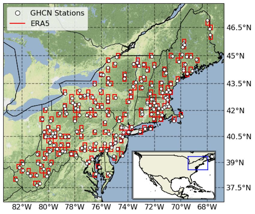
from https://cds.climate.copernicus.eu/cdsapp#!/home. Figure 1 shows the co-location of the 211 GHCN
stations and corresponding ERA5 grid-boxes used in this study. The Northeast matches the definition
of the region in the Fourth National Climate Assessment [23] as the states of Maine, New Hampshire,
Vermont, New York, New Jersey, Connecticut, Massachusetts, Rhode Island, Delaware, Maryland,
West Virginia, and Pennsylvania. The GHCN data are in-situ observational weather stations that
report daily precipitation, whereas the ERA5 data are a gridded reanalysis product with quarter-degree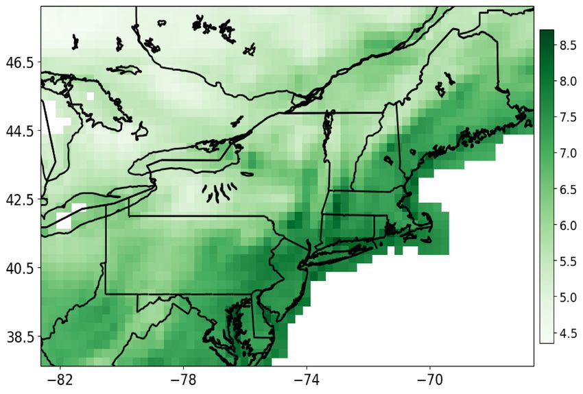
Climate 2020, 8, 148 3 of 14
spatial resolution and hourly temporal resolution. The period of record for this study is from 1979
Climate 2020, 7, x FOR PEER REVIEW 3 of 15
to 2018 to match the start date of ERA5. The 2018 end date was the most recent full-year of ERA5
available at theastime
for the region of data retrieval.
represented by ERA5.Figure 1b showsanalyses
All subsequent the 40-year
weremean daily
carried outprecipitation
using Python forand
the
region
Excel. as represented by ERA5. All subsequent analyses were carried out using Python and Excel.
Figure 1.
Figure 1. (a) Location of
(a) Location of the
the 211 Global Historical
211 Global Historical Climate
Climate Network
Network (GHCN)
(GHCN) precipitation
precipitationstations
stations
(white markers) andand ERA5
ERA5 grid
grid boxes
boxes (red
(red rectangles)
rectangles)used
usedininthis
thisstudy.
study.(b)
(b)Mean
Meanprecipitation
precipitation(mm)
(mm)
of wet
wetdays
days(defined
(defined as days with greater than or equal to 0.33 mm/day, a trace amount
as days with greater than or equal to 0.33 mm/day, a trace amount of precipitation)of
precipitation) in the ERA5 reanalysis
in the ERA5 reanalysis from 1979 to 2018.from 1979 to 2018.
There are a number of types of products available available in in the
the ERA5
ERA5 dataset.
dataset. OneOneof ofthese,
these,the
theERA5
ERA5
surface forecast product, includes two separate initialization times, times, 06 06 UTC
UTCand and18 18UTC.
UTC.Each Eachforecast
forecast
is run for 18 h from the initialization
initialization time,time, resulting
resultingin inaasix-hour
six-houroverlap
overlapbetween
betweenthe thetwo
twoforecasts.
forecasts.
This overlap produces an estimate of model model spin-up
spin-up in in precipitation,
precipitation, which which occurs
occurs as as the
the model
model
adjusts to the assimilation of new data. Over Over ourour domain
domainof of interest,
interest, we we found
foundsix sixpercent
percentmoremore
precipitation
precipitation in the 12–18 h forecasts than the 0–6 h forecasts for the same verification
the 0–6 h forecasts for the same verification time. Therefore, time. Therefore,
to reduce the effects of model spin-up, spin-up, we we combined
combined the the 7–18
7–18hhforecast
forecasthours
hours(valid
(validfor for13–00
13–00UTC)
UTC)
from the 06 UTC analysis, and and thethe 7–18
7–18 hh forecast
forecast hours
hours (valid
(valid forfor 01–12
01–12 UTC)
UTC) from fromthe the1818UTCUTC
analysis. These hourly ERA5 data were aggregated up to the daily time scale
ERA5 data were aggregated up to the daily time scale by summing the hourly by summing the hourly
accumulations from
precipitation accumulations from midnight-to-midnight
midnight-to-midnightlocal localtime,
time,consistent
consistentwith withthe thetime
timeperiod
period
over which the GHCN stations report daily precipitation.
Only GHCN stations with at least least 95%
95% oror greater
greater data
datacoverage
coverageover overtheir
theirperiod
periodof ofrecord
recordwere
were
analysis. For
used in this analysis. For our
our domain
domain of of interest,
interest, 211
211 GHCN
GHCN stationsstations metmet this
this criterion.
criterion. ERA5ERA5isisaa
continuous dataset
continuous dataset with
withno nomissing
missingdata.data.Each
Eachof of
thethe
211211
GHCN GHCN stations waswas
stations thenthenmatched
matchedwithwith
the
ERA5 grid box to which it was closest (Figure 1a). Due to the potential
the ERA5 grid box to which it was closest (Figure 1a). Due to the potential for missing data within for missing data within the
GHCN,
the GHCN,andand
to ensure that that
to ensure the data coverage
the data was was
coverage overover
an identical time time
an identical period for both
period for datasets, any
both datasets,
days that were missing in the GHCN were identified and were removed
any days that were missing in the GHCN were identified and were removed from the matching ERA5 from the matching ERA5
grid box.
grid box. Thus,
Thus, for
for each
each location,
location,we weproduced
producedtwo twodatasets
datasetsof ofmatching
matchingperiod periodofofrecord
recordandandlength.
length.
In the cases where two GHCN stations fell within or were closest to a given ERA5 grid box, thelatter
In the cases where two GHCN stations fell within or were closest to a given ERA5 grid box, the latter
was used
was used as
as the
the match
match forfor both
both stations,
stations, although
although analyses
analyses that that used
useddate datematching
matchingwere wereperformed
performed
separately for
separately for each
each GHCN
GHCN station.
station.
Wet days were defined
Wet days were defined as as those
those on on which
which precipitation
precipitation accumulations
accumulationsrecorded recordedwere wereequal
equalto to
or greater than 0.3 mm/day (i.e., a trace). The GHCN stations only record daily precipitationatator
or greater than 0.3 mm/day (i.e., a trace). The GHCN stations only record daily precipitation or
above aa trace
above trace amount,
amount, whereas
whereas the the ERA5
ERA5 precipitation
precipitation estimates
estimatesare are aa model
model derived
derivedproduct
productthat that
can report accumulations which are smaller than the measurements that
can report accumulations which are smaller than the measurements that could be made by a standard could be made by a standard
precipitation gauge.
precipitation gauge. Therefore,
Therefore, we we removed
removed all all days
days with
with less
less than
thanthisthistrace
traceamount
amountof ofprecipitation
precipitation
from both datasets. It should be noted, however, that although the lengths of record ofwet
from both datasets. It should be noted, however, that although the lengths of record of wetdays
days
produced non-matching datasets, we do not believe that the difference in
produced non-matching datasets, we do not believe that the difference in the number of precipitationthe number of precipitation
days adversely affected the statistical results, due to the length of the period of record and the time
scales considered.
The Atlantic Ocean considerably influences the weather and climate of the nine states in the
Northeast that border it. We determined the distance from the coast to each ERA5 grid box using the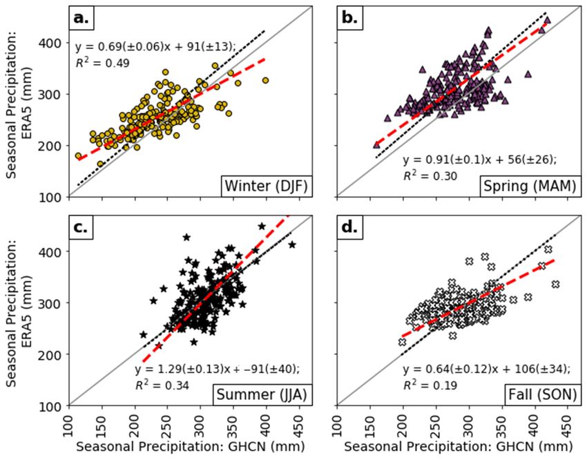
Climate 2020, 8, 148                                                                                 4 of 14

days adversely affected the statistical results, due to the length of the period of record and the time
scales considered.
     The Atlantic Ocean considerably influences the weather and climate of the nine states in the
Northeast that border it. We determined the distance from the coast to each ERA5 grid box using the
ERA5 land-sea mask, a binary variable, where zero represents a “sea” grid point and one represents a
“land” grid point. We used the Haversine formula, which computes the distance on a sphere between
two points from their latitude and longitude, to determine the distance from the coast.
     To examine how well ERA5 represents the heaviest precipitation across the Northeast, we compared
the values of the 90th, 95th, and 99th percentile thresholds of daily precipitation of both datasets as
well as the daily precipitation accumulation above the 90th, 95th, and 99th percentiles of wet day
precipitation [16,24]. We first found the values of the 90th, 95th, and 99th percentiles of wet day
precipitation for both datasets using all 40 years of data for each station. From there, we summed up
the precipitation accumulation for any day with precipitation that fell above the percentile threshold
considered. We did this for every year at each station and its corresponding ERA5 grid box. We then
took the average of this yearly accumulation over a threshold over the 40-year period and used it in
our analyses. We examine not only the thresholds themselves, but also the precipitation accumulation
above these thresholds to get a sense of the average amount of heavy precipitation that falls each year.
     We compared variables using ordinary least squares regression, zero intercept regression,
multiple linear regression, and Deming regression [25]. The latter fits a line to two-dimensional
data where both variables are measured with error (i.e., the line is weighted by the ratio of the variances
of each dataset), and was used because both the ERA5 and GHCN datasets have some form of error,
whether that be model or measurement error.

3. Results
     In the following analyses, all means were taken over the 1979–2018 period of record using a
seasonal or yearly aggregate of daily precipitation accumulations unless otherwise stated. Differences in
precipitation and elevation were always taken as ERA5–GHCN.

3.1. Climate Comparison
      We first computed yearly precipitation totals for each location and each dataset separately,
and then took the mean of those yearly values for both ERA5 and the GHCN. Figure 2a shows that the
relationship between the two datasets is influenced by the highest elevation points (Mounts Washington
and Mansfield in New Hampshire and Vermont, respectively; Table 1). This is not surprising given that
the ERA5 grid boxes are a distributed measure of precipitation over the full quarter-degree grid box,
whereas the actual location of the GHCN precipitation gauges on these two mountain peaks were 949 m
and 678 m above their respective mean grid box elevations. Therefore, these two mountain-top stations
were excluded from subsequent analyses in order to reduce their impact on the results (Figure 2b).
      Figure 2b illustrates that the average yearly precipitation was generally higher in ERA5 than the
GHCN, since more points are above the 1:1 line. The 209-station average of the annual precipitation
ratio (ERA5/GHCN) was 1.06 ± 0.12 (where the ± uncertainty is the standard deviation, here and
throughout the paper), and mean absolute error (MAE) of 109 ± 78 mm/year (Table S1). The average
annual precipitation may be larger in ERA5 due to two reasons: (1) ERA5 on average has 22 ± 6%
more wet days than the GHCN which would result in larger yearly precipitation totals; (2) the GHCN
data have not been corrected for precipitation undercatch. Undercatch in standard precipitation
gauges, primarily due to wind effects, has been well documented as a systematic error in observational
precipitation measurements, especially with snowfall [26,27]. Errors from gauge undercatch can result
in significant underrepresentation of precipitation accumulation at a site, and in this analysis may have
contributed to the smaller yearly precipitation accumulations noted in the GHCN.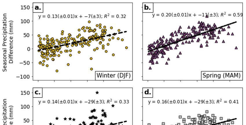
Climate 2020, 7, x FOR PEER REVIEW 5 of 15
in this2020,
Climate analysis
8, 148 may have contributed to the smaller yearly precipitation accumulations noted in
5 ofthe
14
GHCN.
Figure 2.2. (a) Average yearly
Figure yearly precipitation
precipitation ((mm)
((mm) blue
blue circles).
circles). (b) Average yearly
yearly precipitation,
precipitation,
withoutMounts
without MountsWashington
Washingtonand andMansfield
Mansfield((mm)
((mm)blue
blueplus
plussigns).
signs). (c) Precipitation difference
difference (mm)
(mm)
vs. distance
vs. distancefrom
from coast
coast ((km)((km)
blue blue diamonds).
diamonds). (d) Precipitation
(d) Precipitation differencedifference
(mm) vs. (mm) vs. difference
elevation elevation
((m) blue stars).
difference Panels
((m) blue (a,b)Panels
stars). show (a,b)
the reference
show the1:1 line (grey
reference 1:1solid), the zero
line (grey intercept
solid), the zeroregression
intercept
(black dotted)
regression and dotted)
(black Demingand regression
Deming (red dashed and
regression (redequation).
dashed and Panels (c,d) show
equation). ordinary
Panels least
(c,d) show
squares
ordinaryregression (black
least squares dashed).(black dashed).
regression
Table 1. Regression analyses for 1979–2018 annual means.
Figure 2c shows the dependence of the difference in mean yearly precipitation upon the distance
away from the Atlantic Coast, with the linearSlope fit shown Y-Intercept
in Table 1. On the coast,p-Value
R-Squared that difference
on Slope was
−2
−76 ± 11 mmDeming
with aRegression
linear increase
(mm) inland of 62±±0.27
0.66 4 mm* per421100 km. Therefore,
± 294 0.23 by 1201.3km inland
× 10 from
the coast,Zero
theIntercept
ERA5 Regression
precipitation
(mm) was larger
1.02 ±than
0.01 * the GHCN, 0 a value–that continued
1.5 × 10 to increase
−187
inland. ThisRegression
Deming may be (No linked to two
Mountains; reasons:
mm) 0.84 (1) the* spatial
± 0.11 226 ±resolution
117 of ERA5 is2.1
0.23 not sufficient
× 10 −13 to
capture local sea breeze circulations,
Zero Intercept Regression which aid in the production of precipitation along the coast; (2)
1.03 ± 0.01 * 0 – 1.2 × 10−202
ERA5 has more (Noprecipitation
Mountains; mm) inland, possibly a result of the two aforementioned issues regarding the
larger number of wetDifference
Precipitation days in (mm)
ERA5 and the undercatch of−76
0.62 ± 0.04 *
the± GHCN
11
precipitation
0.51
gauges. −33
1.3 × 10
vs. Distance from Coast (km)
Precipitation Difference (mm)
0.57 ± 0.08 * 22 ± 9 0.20 1.04 × 10⁻¹¹
vs. Elevation Difference (m)
* Result is significant to the 95% confidence level.
Figure 2c shows the dependence of the difference in mean yearly precipitation upon the distance
away from the Atlantic Coast, with the linear fit shown in Table 1. On the coast, that difference was
−76 ± 11 mm with a linear increase inland of 62 ± 4 mm per 100 km. Therefore, by 120 km inland from
the coast, the ERA5 precipitation was larger than the GHCN, a value that continued to increase inland.
This may be linked to two reasons: (1) the spatial resolution of ERA5 is not sufficient to capture local
sea breeze circulations, which aid in the production of precipitation along the coast; (2) ERA5 has more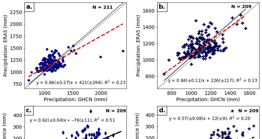
Climate 2020, 8, 148                                                                                          6 of 14

precipitation inland, possibly a result of the two aforementioned issues regarding the larger number of
wet days in ERA5 and the undercatch of the GHCN precipitation gauges.
     The difference in the elevation between the ERA5 grid point and the GHCN station may also
play a role in the differences in precipitation noted between the two datasets. While we treated the
distance from the Atlantic Coast as the same for both ERA5 and the GHCN, the mean elevation of
the grid point and associated station differ. Each GHCN station has a point elevation, while ERA5
has a mean value for the quarter-degree grid box. ERA5 only resolves the mean orography on the
quarter-degree scale, but has additional sub-grid scale orography (at 5000 m resolution) to better
represent the momentum transfers that are influenced by small-scale variations in orography [28].
The full impact of this sub-grid scale orography in regions of complex topography is unclear. The mean
elevation difference between the two datasets was 53 ± 97 m, meaning that, on average, the ERA5 grid
boxes have a higher elevation, although the standard deviation is large. In complex terrain, the GHCN
station may be located preferentially at lower elevations.
     As the elevation difference increases, so too does the difference in precipitation, with a lot of
scatter in this relationship (Figure 2d, Table 1). Since the distance inland from the coast is also
correlated with elevation (but not correlated with elevation difference), the combination of these two
variables showed a clear improvement in the regression results. Using both the distance from the
Atlantic Coast and elevation difference as explanatory variables, for predicting the difference in average
annual precipitation, revealed that the R-squared value for the multiple linear regression increased to
0.60 (Table 2), versus 0.51 and 0.20 for the distance from the Atlantic Coast or the elevation difference,
respectively (Table 1).

      Table 2. Multiple linear regression of average yearly precipitation difference between ERA5 and GHCN
      (mm) on the distance from the coast (km) and elevation difference (m).

                          Slope of the Distance from the            Slope of the Elevation
           Y-Intercept                                                                            R-Squared
                                 Coast (p-Value)                     Difference (p-Value)
             −85 ± 10        0.56 ± 0.04 (1.2 × 10⁻³² ) *          0.40 ± 0.06 (7.8 × 10⁻¹¹ ) *     0.60
                                  * Result is significant to the 95% confidence level.

3.2. Seasonal Analysis
      Understanding how well ERA5 represents precipitation seasonally is also important in determining
its utility for hydrologic studies across the Northeast. Seasons are defined meteorologically as: Winter:
December, January, and February (DJF); Spring: March, April, and May (MAM); Summer: June,
July, and August (JJA); Fall: September, October, and November (SON). We computed the total
precipitation in each season of each year and then took the mean over each season. MAE for seasons
were 31 ± 21 mm, 40 ± 26 mm, 27 ± 22 mm, and 29 ± 19 mm for winter, spring, summer, and fall,
respectively (Table S1). Figure 3 and Table 3 compare these 40-year averages by season for ERA5 and
the GHCN. ERA5 estimates were generally larger in winter, spring (both about 10%), and fall (1%) but
not in summer, illustrated by where the points fell relative to the 1:1 line in Figure 3. The slightly lower
precipitation in ERA5 than the GHCN in summer may be due to the convective parameterization in
ERA5. Convective precipitation is the main mode of precipitation accumulation in the summer in
the Northeast, whereas other larger-scale precipitation-producing systems occur in the other seasons.
All slopes of the Deming regression analysis are less than one, except for in summer, indicating a change
in the ERA5–GHCN relationship during this season (Table 3). Point precipitation accumulations at
individual stations may also be under-sampled given the nature of scattered convective precipitation
compared to large-scale precipitation events.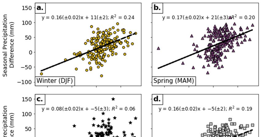
accumulation in the summer in the Northeast, whereas other larger-scale precipitation-producing
 systems occur in the other seasons. All slopes of the Deming regression analysis are less than one,
 except for in summer, indicating a change in the ERA5–GHCN relationship during this season (Table
 3). Point precipitation accumulations at individual stations may also be under-sampled given the
Climate
 nature2020, 8, 148
         of scattered convective precipitation compared to large-scale precipitation events.  7 of 14

    Figure 3. Average seasonal precipitation of ERA5 vs. GHCN (mm) for (a) Winter (yellow circles),
    (b) Spring
     Figure     (purple triangles),
             3. Average             (c) Summer (black
                           seasonal precipitation       stars),
                                                  of ERA5   vs.(d)  Fall (white
                                                                 GHCN     (mm) X’s).
                                                                                for (a)All panels(yellow
                                                                                        Winter    show the  Deming
                                                                                                         circles), (b)
    regression   (red dashed
     Spring (purple            and(c)
                       triangles), equation),
                                      Summer fixed
                                               (blackintercept  regression
                                                       stars), (d)          (black
                                                                   Fall (white  X’s).dotted), andshow
                                                                                      All panels   the reference
                                                                                                        the Deming 1:1
    line (grey solid).
     regression   (red dashed and equation), fixed intercept regression (black dotted), and the reference 1:1
     line (grey solid).
                             Table 3. Regression analyses for the seasonal precipitation.

                                   Season              Slope          Y-Intercept      R-Squared    p-Value on Slope
                                Winter (DJF)        0.69 ± 0.06 *        91 ± 13           0.49         2.1 × 10⁻²⁵
   Seasonal Precipitation:     Spring (MAM)         0.91 ± 0.10 *        56 ± 26           0.30         1.0 × 10⁻¹⁷
    Deming Regression          Summer (JJA)         1.29 ± 0.13 *       −91 ± 40           0.34         7.8 × 10⁻¹⁹
                                 Fall (SON)         0.64 ± 0.12 *       106 ± 34           0.19         3.1 × 10⁻⁷
                                Winter (DJF)        1.06 ± 0.01 *           0               –          1.5 × 10−182
   Seasonal Precipitation:
       Zero Intercept
                               Spring (MAM)         1.09 ± 0.01 *           0               –          5.5 × 10−190
        Regression             Summer (JJA)          1 ± 0.01 *             0               –          5.4 × 10−201
                                 Fall (SON)          1 ± 0.01 *             0               –          1.3 × 10−194
                                Winter (DJF)        0.13 ± 0.01 *        7±3               0.32         8.4 × 10⁻¹⁹
   Seasonal Precipitation
                               Spring (MAM)          0.2 ± 0.01 *        11 ± 3            0.59         1.1 × 10−41
    Difference (mm) vs.
  Distance from Coast (km)     Summer (JJA)         0.14 ± 0.01 *        29 ± 3            0.33         1.2 × 10⁻¹⁹
                                 Fall (SON)         0.16 ± 0.01 *        29 ± 3            0.41         1.8 × 10⁻²⁵
                                Winter (DJF)        0.16 ± 0.02 *        11 ± 2            0.24         4.1 × 10⁻¹⁴
   Seasonal Precipitation
                               Spring (MAM)         0.17 ± 0.02 *        21 ± 3             0.2         1.9 × 10⁻¹¹
    Difference (mm) vs.
  Elevation Difference (m)     Summer (JJA)         0.08 ± 0.02 *        −5 ± 3            0.06         5.0 × 10⁻⁴
                                 Fall (SON)         0.16 ± 0.02 *        −5 ± 2            0.19         2.5 × 10⁻¹¹
                                    * Result is significant to the 95% confidence level.

     Next, we examined the relationship between the difference in the mean seasonal precipitation
totals versus both the distance from the Atlantic Coast and elevation difference using results from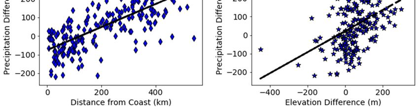
Climate 2020, 8, 148                                                                                                       8 of 14

the ordinary least squares regression analysis. Similar to Figure 2c, linear regressions revealed that
during all seasons, as the station’s distance from the coast increased, the difference in average seasonal
precipitation shifted from a negative or near zero value near the coast to a linear increase inland
(Figure 4). The transition from a negative precipitation difference (ERA5 < GHCN) to a positive one
(ERA5 > GHCN) occurred around 50 km inland from the coast in winter and spring, and around 200 km
inland in the summer and fall. Higher precipitation totals along the coast in summer may have been
due to the frequency of sea breezes. While Barbato [29] and Sikora et al. [30] found a peak sea-breeze
frequency from June to August at Boston, Massachusetts and the Chesapeake Bay region in Maryland
(both on the Atlantic Coast), Defant [31] found that the strongest sea breezes at mid-latitude coastal
locations tend to occur in summer. Spring and summer exhibit large thermal gradients from the sea to
the land which produce sea breezes. The scatterplots and regression results (R-squared values) for the
winter, spring, and fall of the difference in seasonal precipitation and elevation difference (Figure 5)
closely resembled those for the full-year analyses shown in Figure 2d and Table 1. Summer results
showed a much smaller dependence on elevation difference and variance explained as compared to
the values in Figure 3c (Figure 5c and Table 3).
 Climate 2020, 7, x FOR PEER REVIEW                                                                                         9 of 15

       Figure4.4.The
      Figure      Thedifference
                       differenceininthe
                                       the average
                                         average     seasonal
                                                  seasonal     precipitation
                                                            precipitation   (mm)(mm)
                                                                                   vs. vs. distance
                                                                                        distance  from from   the coast
                                                                                                         the coast  (km)(km)
                                                                                                                         for
       forWinter
      (a)  (a) Winter  (yellow
                  (yellow        circles),
                           circles),       (b) Spring
                                     (b) Spring        (purple
                                                 (purple        triangles),
                                                          triangles),         (c) Summer
                                                                       (c) Summer      (black(black
                                                                                               stars),stars), (d)(white
                                                                                                       (d) Fall   Fall (white
                                                                                                                        X’s).
      All panels
       X’s).      show the
             All panels show ordinary   least squares
                               the ordinary            regression
                                               least squares        (black (black
                                                              regression    line and   equation).
                                                                                    line and equation).

     Table 4 summarizes the results of the multiple linear regression of the mean seasonal precipitation
difference on both the distance from the Atlantic Coast and the elevation difference. For all seasons,
the multiple linear regression yielded a higher amount of variance explained than did the ordinary
linear regression (Tables 3 and 4). The relationship with the distance from the Atlantic Coast was
weakest in the winter and strongest in the spring, where the latter season also had the largest R-squared
Climate 2020, 8, 148 9 of 14
value. This again suggests the importance of a high frequency of sea breezes along the coast in the
spring. Elevation differences are equally important in winter, spring, and fall, but negligible in summer,
consistent with the results of the ordinary linear regression (Tables 3 and 4). Increases in the R-squared
values in the multiple linear regression for all seasons, confirm that the coastal distance and elevation
difference should not be considered individually as explanatory variables.
Climate 2020, 7, x FOR PEER REVIEW 10 of 15
Figure5.5. The
Figure The difference in thethe average
averageseasonal
seasonalprecipitation
precipitation(mm)(mm)vs.vs.elevation
elevationdifference (m)
difference forfor
(m) (a)
Winter (yellow circles), (b) Spring (purple triangles), (c) Summer (black stars), (d) Fall (white
(a) Winter (yellow circles), (b) Spring (purple triangles), (c) Summer (black stars), (d) Fall (white X’s).X’s). All
panels
All show
panels showthethe
ordinary least
ordinary squares
least regression
squares (black
regression line
(black and
line equation).
and equation).
Table 4 summarizes the results of the multiple linear regression of the mean seasonal
Table 4. Multiple linear regression of the mean seasonal precipitation difference between ERA5 and
precipitation difference on both the distance from the Atlantic Coast and the elevation
GHCN (mm) on the distance from the coast (km) and elevation difference (m).
difference. For all seasons, the multiple linear regression yielded a higher amount of variance
explained than did the ordinary linear Sloperegression
of the Distance(Tables 3 and 4). The relationship with the
Slope of the Elevation
Season
distance Y-Intercept
from the Atlantic from the in
Coast was weakest Coast
the winter and strongest R-Squared
in the spring, where
Difference (p-Value)
(p-Value)
the latter season also had the largest R-squared value. This again suggests the importance of a
(DJF) of sea−10 ± 3 along −17 ) * × 10−12 ) * are equally
highWinter
frequency breezes 0.11the± 0.01 × 10
(6.0 in
coast the ± 0.02 (2.8differences
0.13Elevation
spring. 0.46
Spring (MAM) −13 ± 3 −41 −11 ) *
0.18 ± 0.1 (1.3
important in winter, spring, and fall, but negligible −18 × 10 ) * 0.11 ± 0.02 (1.7
in summer, consistent with × 10 the results0.67
of the
Summer (JJA) −30 ± 3 0.13 ± 0.1 (7.0 × 10 ) * 0.04 ± 0.02 (3.6 × 10⁻² ) * 0.34
ordinary linear regression (Tables 3 and 4). Increases in the R-squared values in the multiple
Fall (SON) −31 ± 3 0.14 ± 0.01 (1.0 × 10⁻²³ ) * 0.11 ± 0.02 (1.4 × 10⁻⁹ ) * 0.51
linear regression for all seasons, confirm that the coastal distance and elevation difference should
* Result is significant to the 95% confidence level.
not be considered individually as explanatory variables.
Table 4. Multiple linear regression of the mean seasonal precipitation difference between ERA5 and
GHCN (mm) on the distance from the coast (km) and elevation difference (m).
Slope of the Elevation
Season Y-Intercept Slope of the Distance from the Coast (p-Value) R-Squared
Difference (p-Value)
Winter (DJF) −10 ± 3 0.11 ± 0.01 (6.0 × 10−17) * 0.13 ± 0.02 (2.8 × 10−12) * 0.46
Spring (MAM) −13 ± 3 0.18 ± 0.1 (1.3 × 10−41) * 0.11 ± 0.02 (1.7 × 10−11) * 0.67
Summer (JJA) −30 ± 3 0.13 ± 0.1 (7.0 × 10−18) * 0.04 ± 0.02 (3.6 × 10−2) * 0.34
Fall (SON) −31 ± 3 0.14 ± 0.01 (1.0 × 10−23) * 0.11 ± 0.02 (1.4 × 10−9) * 0.51Climate 2020, 8, 148 10 of 14
3.3. Heavy Precipitation
We compared heavy precipitation statistics across the Northeast between ERA5 and the GHCN.
Table 5 summarizes the value of the 90th, 95th, and 99th percentiles of daily precipitation between the
two datasets, as well as the sum of precipitation over these percentiles. Given the similarity in the
results for the three thresholds (Table 5), only the 90th percentile value will be discussed here. Plots for
the 95th and 99th percentile thresholds can be found in the Supplementary Materials (Figures S1 and
S2, respectively).
Table 5. Regression analyses for heavy precipitation.
Percentile
Slope Y-Intercept R-Squared p-Value on Slope
Threshold
Value of Percentile 90th 0.50 ± 0.02 * 7 ± 0.4 0.81 6.5 × 10−77
Threshold: 95th 0.50 ± 0.02 * 9 ± 0.5 0.82 4.2 × 10−79
ERA5 vs. GHCN (mm) 99th 0.44 ± 0.02 * 17 ± 0.9 0.78 1.3 × 10−70
Precipitation Above 90th 0.63 ± 0.09 * 176 ± 41 0.26 1.4 × 10⁻¹¹
Threshold: Deming 95th 0.59 ± 0.09 * 121 ± 27 0.24 2.0 × 10⁻⁹
Regression 99th 0.53 ± 0.11 * 41 ± 10 0.14 4.5 × 10⁻⁶
Precipitation Above 90th 1 ± 0.01 * 0 – 3.1 × 10−204
Threshold: Zero 95th 0.98 ± 0.01 * 0 – 3.3 × 10−201
Intercept Regression 99th 0.95 ± 0.01 * 0 – 5.7 × 10−187
Precipitation Difference 90th 0.23 ± 0.02 * −44 ± 5 0.42 5.5 × 10⁻²⁶
Above Threshold (mm) vs. 95th 0.15 ± 0.01 * −3 ± 3 0.39 3.8 × 10⁻²⁴
Distance from Coast (km) 99th 0.05 ± 0.00 * −15 ± 1 0.38 2.1 × 10⁻²³
Precipitation Difference 90th 0.26 ± 0.03 * −10 ± 3 0.25 2.3 × 10⁻¹⁴
Above Threshold (mm) vs. 95th 0.17 ± 0.02 * −11 ± 2 0.26 5.7 × 10⁻¹⁵
Elevation Difference (m) 99th 0.06 ± 0.01 * −7 ± 1 0.26 1.8 × 10⁻¹⁵
* Result is significant to the 95% confidence level.
Figure 6a summarizes the values of the 90th percentile thresholds for the two datasets. For the
stations considered, the 90th percentile threshold value for the GHCN was greater than that for
ERA5, since all of the points are below the 1:1 line (Figure 6a; MAE of 4 ± 2 mm, Table S1).
However, the precipitation accumulation above the 90th percentile showed that the GHCN dataset
did not have consistently higher precipitation accumulations than did the ERA5 dataset, as the
zero-intercept regression line corresponds with the 1:1 line (Figure 6b; MAE 44 ± 41 mm, Table S1).
Comparing histograms of the frequency of days with less than 10.3 mm/day of precipitation illustrates
that there were many more days with small precipitation accumulations in ERA5 relative to the GHCN
(Figure S3). The large number of smaller precipitation values in ERA5 contributed to a lower threshold
value when compared to the GHCN due to the higher density of the left tail of the histogram. The value
of precipitation that fell above that threshold is dependent upon individual station characteristics and
daily precipitation distributions which led to both larger and smaller accumulations above the 90th
percentile threshold for ERA5 (Figure 6b). The Deming regression slopes are less than one, similar to
most earlier plots, decreasing slightly from the 90th to 99th percentile thresholds. Conceptually,
these slopes mean that for lower precipitation values, ERA5 was greater than the GHCN, while for
higher precipitation values, the GHCN was greater than ERA5. The scatterplot of the difference in the
precipitation accumulation above the 90th percentile between ERA5 and the GHCN against the distance
from the Atlantic Coast (Figure 6c) resembled those of Figures 2c and 4, where ERA5 consistently
showed less precipitation along the coast. Figure 6d shows that the difference in the precipitation
above the 90th percentile generally increased with the difference in elevation, also shown in the
seasonal and full-year analyses (Figures 2d and 5). As aforementioned, the distance from the coast and
elevation difference cannot be considered individually as explanatory variables. Table 6 summarizes
the multiple linear regression results of the precipitation accumulation difference above the 90th, 95th,Climate 2020, 7, x FOR PEER REVIEW 12 of 15
Distance from Coast
Climate 2020, 8,(km)
148 11 of 14
Precipitation 90th 0.26 ± 0.03 * −10 ± 3 0.25 2.3 × 10⁻¹⁴
Difference Above 95th from0.17
and 99th percentiles on both distance the ±Atlantic
0.02 * Coast−11 ± 2elevation0.26
and 5.7 ×percentile
difference. All 10−15
Threshold (mm) vs.
thresholds have a similar explained variance. The dependence on the distance from the coast and
Elevation Difference 99th 0.06 ± 0.01 * −7 ± 1 0.26
the elevation difference also had similar slopes, but the actual slopes decreased from the1.8 × 10−15
90th to 99th
(m)
percentile thresholds.
* Result is significant to the 95% confidence level
Figure6.6.(a)
Figure (a)The
The90th
90thpercentile
percentileprecipitation
precipitationthreshold
threshold ((mm)
((mm) purple x’s), (b) precipitation
precipitation above
above the
the
90thpercentile
90th percentile ((mm)
((mm) purple
purple circles),
circles), (c) precipitation
(c) precipitation difference
difference overpercentile
over 90th 90th percentile
(mm) vs.(mm) vs.
distance
distance
from coast from
((km)coast
purple((km) purple diamonds),
diamonds), (d) precipitation
(d) precipitation difference
difference over over 90th
90th percentile percentile
(mm) (mm)
vs. elevation
vs. elevation
difference ((m)difference ((m) purple
purple stars). Panel stars). Panelthe
(b) shows (b)reference
shows the1:1reference 1:1 line
line (grey (grey
solid), thesolid), the zero-
zero-intercept
intercept (black
regression regression (black
dotted), anddotted), and the
the Deming Deming(red
regression regression
dashed(redand dashed
equation).andPanels
equation).
(a,c,d)Panels
show
(a,c,d) show
ordinary ordinary
regression regression
(black dashed).(black dashed).
Table Multiple
6. 6.
Table linear
Multiple regression
linear of the
regression difference
of the of precipitation
difference accumulation
of precipitation on the
accumulation ondistance from
the distance
the coast (km), and elevation difference (m) at the 90th, 95th, and 99th percentiles thresholds (mm).
from the coast (km), and elevation difference (m) at the 90th, 95th, and 99th percentiles thresholds
(mm).
Slope of the Distance Slope of the Elevation
Threshold Y-Intercept R-Squared
Slope of the Distance from the Difference
from the Coast (p-Value) Slope of the(p-Value)
Elevation
Threshold Y-Intercept R-Squared
90th Percentile −48 ± 4 0.20 ± Coast (p-Value)
0.02 (6.2 × 10⁻²⁵ ) * 0.19Difference
± 0.03 (2.3(p-Value)
× 10−13 ) * 0.55
95th90th Percentile −48±±34 0.13 ± 0.01 (5.3 × ×1010−23)) **
0.20 ± 0.02 (6.2 0.13 ± 0.02 (7.3 ××10
0.19 ± 0.03 (2.3 10−14 ))** 0.55
−25 −13
Percentile −35 0.54
95th Percentile
99th Percentile −35±±13
−16 0.05 ± 0.004 (2.8 × 10 ))**
0.13 ± 0.01 (5.3 × 10 −23
−22 0.05 ± 0.01 (2.2 × 10 ))**
0.13 ± 0.02 (7.3 × 10 −14
−14 0.54
0.54
99th Percentile −16 ± 1 0.05 ± 0.004 (2.8 × 10−22) * 0.05 ± 0.01 (2.2 × 10−14) * 0.54
* Result is significant to the 95% confidence level.
* Result is significant to the 95% confidence level.
4. Discussion and Conclusions
The comparison of the yearly precipitation accumulation from the ERA5 climate reanalysis against
that from GHCN stations across the Northeast provides a framework for assessing the value of ERA5Climate 2020, 8, 148 12 of 14
for different applications in the Northeast. Several key patterns emerged. Average annual precipitation
was generally higher in ERA5 than in the GHCN. The 209-station average of the annual precipitation
ratio (ERA5/GHCN) was 1.06 ± 0.12. This may be due to the 22 ± 6% more wet days in ERA5, or that
the GHCN data have not been corrected for precipitation undercatch. We found a relationship between
precipitation differences and both the distance from the Atlantic Coast and the difference in elevation.
ERA5 consistently displayed less precipitation both along the coast and for isolated mountain peaks.
Coastal precipitation shortfalls probably reflected the inability of the ERA5 parameterization to quantify
sea breeze-induced precipitation at the quarter-degree spatial resolution. In regions of high terrain,
ERA5 cannot resolve mountain peaks that are well above the mean grid elevation. When considered
together, the distance from the coast and elevation difference provided a better fit to the differences in
precipitation, implying that they should not be treated independently.
Seasonally, ERA5 showed 10% more precipitation than the GHCN in winter and spring, 1% in
autumn and a trace less in summer. Similar patterns were observed in the relationship between distance
from the coast and elevation difference in all seasons except summer, which was the only season
in which ERA5 did not have more precipitation than the GHCN and the relationship between the
difference in precipitation and the elevation difference was the weakest. We attributed these differences
in the summer months to the frequency of convective precipitation events, which are parameterized
in ERA5.
The forty-year 90th, 95th, and 99th percentile thresholds for daily heavy precipitation were well
correlated, and the mean precipitation accumulation over these percentiles was very similar for both
ERA5 and the GHCN. The structure of the heavy precipitation dependence on the distance from the
coast and the elevation difference were similar to the long-term and seasonal results suggesting that
the ERA5 dataset will be useful for studies of daily heavy precipitation events.
In assessing the utility of the ERA5 climate reanalysis at aggregated timescales, our study results
highlight the importance of a full appreciation of the strengths and limitations of precipitation estimates
being used in models to explore biogeophysical processes across the landscape. Precipitation datasets
derived primarily from in-situ stations often lack uniform spatial and temporal coverage or require
large interpolation distances in order to create uniform coverage. Such limitations have prompted the
use of climate reanalyses, such as ERA5, which with its quarter-degree spatial and hourly temporal
resolutions, we have shown to be comparable to GHCN observations of precipitation across the
Northeast. The ability to utilize a full coverage, spatio-temporally consistent product such as ERA5
will allow users the increased capability to model or predict land-surface processes across large
geographic regions with greater confidence. There are two important caveats. The first is the biases
that exist in the ERA5 precipitation estimates in terms of their distance from the Atlantic coast and
elevation difference relative to the point GHCN observations. Secondly, we acknowledge that hourly
precipitation estimates, especially the extremes in heavy precipitation, can have significant impacts
on engineering, hydrologic, and agricultural systems (i.e., stormwater, flood control, etc.), and may
not have been represented in our aggregated approach. Therefore, future work should include an
examination of how well ERA5 data represent precipitation at the hourly scale to assess its utility in
applications that require high temporal resolutions.
Supplementary Materials: The following are available online at http://www.mdpi.com/2225-1154/8/12/148/s1,
Table S1: Summary table of comparison metrics between ERA5 and the GHCN, Figure S1: Results from the 40-year
analysis of the 95th Percentile of daily precipitation and accumulation above that threshold, Figure S2: Results
from the 40-year analysis of the 99th Percentile of daily precipitation and accumulation above that threshold,
Figure S3: Distribution of Daily Precipitation Values for ERA5 and the GHCN.
Author Contributions: Conceptualization, C.C.C., A.K.B., L.-A.L.D.-G. and A.B.; data curation, C.C.C.; formal analysis,
C.C.C.; funding acquisition, A.B.; investigation, C.C.C.; methodology, A.K.B.; project administration, A.B.; software,
C.C.C.; supervision, L.-A.L.D.-G. and Arne Bomblies; validation, A.K.B.; visualization, C.C.C.; writing—original draft,
C.C.C.; writing—review and editing, C.C.C., A.K.B., L.-A.L.D.-G. and A.B. All authors have read and agreed to the
published version of the manuscript.Climate 2020, 8, 148 13 of 14
Funding: This material is based upon work supported by the National Science Foundation under VT EPSCoR
Grant No. NSF OIA 1556770.
Acknowledgments: We acknowledge the invaluable advice and assistance we received from ECMWF especially
Hans Hersbach, Gianpaolo Balsamo, and Anton Beljaars.
Conflicts of Interest: The authors declare no conflict of interest.
References
1. Peel, M.C.; Finlayson, B.L.; McMahon, T.A. Updated world map of the Ko ppen-Geiger climate classification.
Hydrol. Earth Syst. Sci. 2007, 11, 1633–1644. [CrossRef]
2. Oswald, E.M.; Dupigny-Giroux, L.A. On the Availability of High-Resolution Data for Near-Surface Climate
Analysis in the Continental U.S. Geogr. Compass 2015, 9, 617–636. [CrossRef]
3. Thornton, P.E.; Running, S.W.; White, M.A. Generating Surfaces of Daily Meteorological Variables over Large
Regions with Complex Terrain. J. Hydrol. 1997, 190, 214–251. [CrossRef]
4. Livneh, B.; Rosenberg, E.A.; Lin, C.; Nijssen, B.; Mishra, V.; Andreadis, K.M.; Maurer, E.P.; Lettenmaier, D.P.
A long-term hydrologically based dataset of land surface fluxes and states for the conterminous United
States: Update and extensions. J. Clim. 2013, 26, 9384–9392. [CrossRef]
5. Maurer, E.P.; Wood, A.W.; Adam, J.C.; Lettenmaier, D.P.; Nijssen, B.A. Long-Term Hydrologically Based
Dataset of Land Surface Fluxes and States for the Conterminous United States. J. Clim. 2002, 15, 3237–3251.
[CrossRef]
6. Daly, C.; Halbleib, M.; Smith, J.I.; Gibson, W.P.; Doggett, M.K.; Taylor, G.H.; Curtis, J.; Pasteris, P.P.
Physiographically sensitive mapping of climatological temperature and precipitation across the conterminous
United States. Int. J. Climatol. 2008, 28, 2031–2064. [CrossRef]
7. Hersbach, H.; Dee, D. ERA5 Reanalysis Is in Production, ECMWF Newsletter 41; ECMWF: Reading, UK, 2016.
8. Dee, D.P.; Uppala, S.M.; Simmons, A.J.; Berrisford, P.; Poli, P.; Kobayashi, S.; Andrae, U.; Balmaseda, M.A.;
Balsamo, G.; Bauer, P.; et al. The ERA-Interim reanalysis: Configuration and performance of the data
assimilation system. Q. J. R. Meteorol. Soc. 2011, 137, 553–597. [CrossRef]
9. Betts, A.K.; Chan, D.Z.; Desjardins, R.L. Near-Surface Biases in ERA5 Over the Canadian Prairies.
Front. Environ. Sci. 2019, 7, 129. [CrossRef]
10. Tarek, M.; Brissette, F.P.; Arsenault, R. Evaluation of the ERA5 reanalysis as a potential reference dataset for
hydrological modelling over North America. Hydrol. Earth Syst. Sci. 2020, 24, 2527–2544. [CrossRef]
11. Beck, H.E.; Pan, M.; Roy, T.; Weedon, G.P.; Pappenberger, F.; Van Dijk, A.I.J.M.; Huffman, G.J.; Adler, R.F.;
Wood, E.F. Daily evaluation of 26 precipitation datasets using Stage-IV gauge-radar data for the CONUS.
Hydrol. Earth Syst. Sci. 2019, 23, 207–224. [CrossRef]
12. Gupta, H.V.; Kling, H.; Yilmaz, K.K.; Martinez, G.F. Decomposition of the mean squared error and NSE
performance criteria: Implications for improving hydrological modelling. J. Hydrol. 2009, 377, 80–91.
[CrossRef]
13. Kling, H.; Fuchs, M.; Paulin, M. Runoff conditions in the upper Danube basin under an ensemble of climate
change scenarios. J. Hydrol. 2012, 424–425, 264–277. [CrossRef]
14. Huffman, G.J.; Bolvin, D.T.; Braithwaite, D.; Hsu, K.; Joyce, R.; Kidd, C.; Nelkin, E.J.; Xie, P. Global Precipitation
Measurement (GPM) Integrated Multi-Satellite Retrievals for GPM (IMERG); NASA: Greenbelt, MD, USA, 2014.
15. Huffman, G.J.; Bolvin, D.T.; Nelkin, E.J. Integrated Multi-Satellite Retrievals for GPM (IMERG) Technical
Documentation, Tech. Rep.; NASA: Greenbelt, MD, USA, 2018.
16. Huang, H.; Winter, J.M.; Osterberg, E.C.; Horton, R.M.; Beckage, B. Total and Extreme Precipitation Changes
over the Northeastern United States. J. Hydrometeorol. 2017, 18, 1783–1798. [CrossRef] [PubMed]
17. Marquardt Collow, A.B.; Bosilovich, M.G.; Koster, R.D. Large-Scale Influences on Summertime Extreme
Precipitation in the Northeastern United States. J. Hydrometeorol. 2016, 17, 3045–3061. [CrossRef] [PubMed]
18. Frei, A.; Kunkel, K.E.; Matonse, A. The Seasonal Nature of Extreme Hydrological Events in the Northeastern
United States. J. Hydrometeorol. 2015, 16, 2065–2085. [CrossRef]
19. Guilbert, J.; Betts, A.K.; Rizzo, D.M.; Beckage, B.; Bomblies, A. Characterization of increased persistence
and intensity of precipitation in the northeastern United States. Geophys. Res. Lett. 2015, 42, 1888–1893.
[CrossRef]Climate 2020, 8, 148 14 of 14
20. Hayhoe, K.; Wake, C.P.; Huntington, T.G.; Luo, L.; Schwartz, M.D.; Sheffield, J.; Wood, E.; Anderson, B.;
Bradbury, J.; DeGaetano, A.; et al. Past and future changes in climate and hydrological indicators in the US
Northeast. Clim. Dyn. 2007, 28, 381–407. [CrossRef]
21. Menne, M.J.; Durre, I.; Vose, R.S.; Gleason, B.E.; Houston, T.G. An overview of the global historical climatology
network-daily database. J. Atmos. Ocean. Technol. 2012, 29, 897–910. [CrossRef]
22. Copernicus Climate Change Service (C3S). ERA5: Fifth Generation of ECMWF Atmospheric Reanalyses of
the Global Climate; Copernicus Climate Change Service Climate Data Store (CDS), 2017; Available online:
https://cds.climate.copernicus.eu/#!/home (accessed on 27 November 2020).
23. Dupigny-Giroux, L.; Mecray, E.L.; Lemcke-Stampone, M.D.; Hodgkins, G.A.; Lentz, E.E.; Mills, K.E.;
Lane, E.D.; Miller, R.; Hollinger, D.Y.; Solecki, W.D.; et al. Northeast. In Impacts, Risks, and Adaptation in the
United States: Fourth National Climate Assessment; U.S. Global Change Research Program: Washington, DC,
USA, 2018; Volume II, pp. 669–742. [CrossRef]
24. Walsh, J.; Wuebbles, D.; Hayhoe, K.; Kossin, J.; Kunkel, K.; Stephens, G.; Thorne, P.; Vose, R.; Wehner, M.;
Willis, J.; et al. Our changing climate. Climate change impacts in the United States. In The Third National
Climate Assessment; U.S. National Climate Assessment: Washington, DC, USA, 2014.
25. Deming, W.E. Statistical Adjustment of Data; Wiley: Hoboken, NJ, USA, 1943.
26. Groisman, P.Y.; Easterling, D.R. Variability and Trends of Total Precipitation and Snowfall over the United
States and Canada. J. Clim. 1994, 7, 184–205. [CrossRef]
27. Groisman, P.Y.; Legates, D.R. The Accuracy of United States Precipitation Data. Bull. Am. Meteorol. Soc. 1994,
75, 215–227. [CrossRef]
28. European Centre for Medium-Range Weather Forecasts (ECMWF). IFS Documentation CY46r1 Part IV: Physical
Processes; ECMWF: Reading, UK, 2019.
29. Barbato, J.P. Areal parameters of the Sea Breeze and Its vertical structure in the Boston Basin. Bull. Am.
Meteorol. Soc. 1978, 59, 1420–1431. [CrossRef]
30. Sikora, T.D.; Young, G.S.; Bettwy, M.J. Analysis of the Western Shore Chesapeake Bay Breeze. Natl. Weather Dig.
2010, 34, 55–65.
31. Defant, F. Local Winds; Malone, T., Ed.; American Meteorological Society: Boston, MA, USA, 1951.
Publisher’s Note: MDPI stays neutral with regard to jurisdictional claims in published maps and institutional
affiliations.
© 2020 by the authors. Licensee MDPI, Basel, Switzerland. This article is an open access
article distributed under the terms and conditions of the Creative Commons Attribution
(CC BY) license (http://creativecommons.org/licenses/by/4.0/).You can also read