Radar Rainfall Estimation in Morocco: Quality Control and Gauge Adjustment - MDPI
←
→
Page content transcription
If your browser does not render page correctly, please read the page content below
hydrology
Article
Radar Rainfall Estimation in Morocco: Quality
Control and Gauge Adjustment
Zahra Sahlaoui 1,2, *       and Soumia Mordane 1
    1   LPPPC, Faculty of Sciences Ben M’Sik, University Hassan II, Casablanca 20085, Morocco;
        mordanesoumia@yahoo.fr
    2   CNRMSI, Direction de la Météorologie National, Casablanca 20240, Morocco
 *      Correspondence: sahlaoui_zahra@yahoo.fr; Tel.: +212-6-66820665

    Received: 25 April 2019; Accepted: 19 May 2019; Published: 23 May 2019

    Abstract: This study focused on investigating the impact of gauge adjustment on the rainfall
    estimate from a Moroccan C-band weather radar located in Khouribga City. The radar reflectivity
    underwent a quality check before deployment to retrieve the rainfall amount. The process consisted
    of clutter identification and the correction of signal attenuation. Thereafter, the radar reflectivity
    was converted into rainfall depth over a period of 24 h. An assessment of the accuracy of the radar
    rainfall estimate over the study area showed an overall underestimation when compared to the rain
    gauges (bias = −6.4 mm and root mean square error [RMSE] = 8.9 mm). The adjustment model
    was applied, and a validation of the adjusted rainfall versus the rain gauges showed a positive
    impact (bias = −0.96 mm and RMSE = 6.7 mm). The case study conducted on December 16, 2016
    revealed substantial improvements in the precipitation structure and intensity with reference to
    African Rainfall Climatology version 2 (ARC2) precipitations.

    Keywords: Moroccan weather radar; rainfall estimate; gauge adjustment; quality control; clutter;
    signal attenuation; ARC2

1. Introduction
     Weather hazards, such as heavy rainfall, have a direct impact on human activity, the economy,
and safety. In fact, floods are the most widespread and harmful weather-related natural disasters.
Therefore, high-resolution precipitation estimates and forecasts are of significant interest for use in
hydrological applications, especially in relation to hilly terrain [1–4]. In numerical weather predictions
(NWP), scientists are deploying several efforts to improve the ability of their models to forecast heavy
rain events [5–7]. As shown by Lopez [8,9] and others [10,11], the assimilation of rainfall measurements
in the preparation of accurate initial atmospheric conditions in NWP models has a positive impact.
     The standard method of collection for quantifying rainfall on the ground is a rain gauge. However,
a gauge is often insufficient because of the high spatial and temporal variability of rainfall, especially in
low-density gauge networks. Thus, radar data is widely used to produce a quantitative precipitation
estimation (QPE). Owing to their large coverage, high spatial resolution and temporal frequency,
weather radars produce observations that adequately represent precipitation structure and evolution.
Nevertheless, these radar measurements have limitations [12] that negatively affect the quality of the
radar QPE [13,14], such as:

•       Beam blockage by obstacles, such as buildings, trees, or mountains, which constitute a mask
        preventing rain detection.
•       Overshooting and partial beam filling, due to the increase of the sounded volume and beam
        altitude at key distances from the radar. This might lead to underestimation of rain intensity.

Hydrology 2019, 6, 41; doi:10.3390/hydrology6020041                             www.mdpi.com/journal/hydrology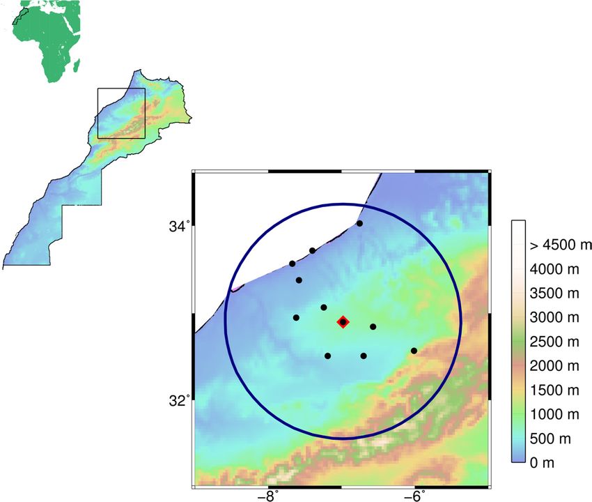
Hydrology 2019, 6, 41                                                                               2 of 13

•     Clutter, such as echoes from non-meteorological targets like airplanes, birds, insects, and dust
      particles, which could result in unrealistic precipitation estimations.
•     Attenuation of the radar signal, which is the gradual loss of power that occurs during heavy rain.
      This effect is more important for radars with short wavelengths (e.g., C-band and X-band radars).

      Therefore, if a QPE with high precision is required from radar data, it is necessary to develop
robust algorithms that deal with these influencing factors, especially clutter and signal attenuation
effects [15].
      There have been several attempts to combine rain gauges and radar data to enhance the quality
of radar rainfall estimates [16–18]. Goudenhoofdt and Delobbe [19] provide a global overview and
evaluation of these merging methods. Several national weather services around the world [20–22]
produce QPEs based on radar and other data sources like gauges, satellites, and NWP models.
      In Morocco, the Moroccan national meteorological service in Khouribga City implemented the
first weather radar in 1985. Since 2013, the meteorological service has modernized its weather radar
network and it now runs six single-polarization C-band Doppler radars and one dual-polarization
C-band Doppler radar [23]. All the radars operate at a range of 250 km, where the radar network
enables nowcasting of weather phenomena related to precipitation. Moreover, for QPE, the service has
deployed Moroccan weather radars. However, there is an underestimation of the radar QPE when
compared to the rain gauge network. Additionally, other weather radar networks worldwide [16] have
observed this radar measurement deficiency.
      Consequently, one should recognize that a comparison between rain gauges and radar QPEs is not
a trivial topic. First, rain gauges provide amounts relative to point accumulations (around 200 cm2 );
whilst the radar QPE corresponds to a volume-averaged rainfall rate. Second, differences between
gauge amounts and radar QPEs not only depend on the quality of radar measurements, but also on the
quality of the rain gauge data and the density of the network. Therefore, to improve the quality of
radar rainfall estimates using a rain gauge depends on good quality gauge data and well-validated
merging methods.
      In the current work, we present an approach for radar rainfall estimation using the Moroccan
C-band radar. First, the radar reflectivity was quality controlled to filter clutter and to correct signal
attenuations. Following that, we applied a mixed adjustment model combining radar rainfall and
gauge measurements. We also applied the method to 10 rainfall events from November–December
2016, and in January 2017. In our study area, this period corresponded to the winter season—being the
rainy season—characterized by an arid to semi-arid climate, with the average annual precipitation
amount ranging from 200 mm to 500 mm.
      An overview of the radar and the gauge network used is in Section 2. Section 2 also provides an
exhaustive description of the data processing and mixed adjustment models. Section 3 presents and
discusses the results, while Section 4 provides the conclusion, along with future areas for development.

2. Materials and Methods

2.1. Data Description

2.1.1. C-Band Radar of Khouribga City
     The radar data used in the current study were from an operational single-polarization C-band
Doppler radar located in Khouribga City (Figure 1). See Table 1 for further details.
     The radar data are used for nowcasting and posterior analysis of extreme weather events over the
plains in both the north and west areas of the radar. The southeast area of the radar is covered by the
Atlas Mountains, which causes a severe beam blockage. Since the estimation can be very inaccurate at
large distances from the radar, a maximum range of 150 km was used [24].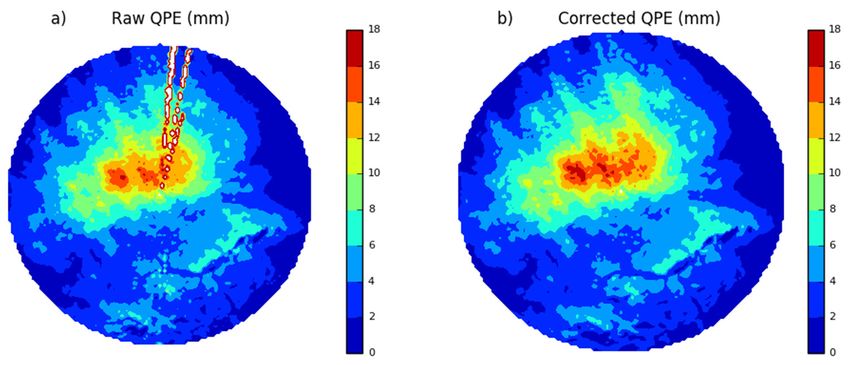
Elevations                        0;0.5;1;1.5;2;3;4;9;15;20°
                                Scanning interval                             10 min

           The radar data are used for nowcasting and posterior analysis of extreme weather events over
Hydrology 2019, 6, in
     the  plains    41 both the north and west areas of the radar. The southeast area of the radar is covered by3 of 13
     the Atlas Mountains, which causes a severe beam blockage. Since the estimation can be very
     inaccurate at large distances from the radar, a maximum range of 150 km was used [24].

     Figure  1. Study
          Figure        area, area,
                   1. Study   including  orography.
                                    including         The blue
                                               orography.         circlecircle
                                                             The blue    represents  Khouribga
                                                                               represents         City’s
                                                                                           Khouribga      radarradar
                                                                                                        City’s  coverage
     at 150  km, the
          coverage      red km,
                     at 150  diamond
                                the red refers
                                        diamondto refers
                                                  the radar’s    location,
                                                         to the radar’s      whilst
                                                                        location,    the the
                                                                                  whilst  black  dots
                                                                                             black dotsindicate
                                                                                                        indicate the
                                                                                                                 the rain
          rainlocation.
     gauges     gauges location.

                        Table 1. Technical specifications of the Khouribga City radar.
     2.1.2. Rain Gauge Network
          The study area comprisedParameter
                                      a gauge network containing 11 stations,
                                                                         Value as shown in Figure 1. A 24 h
     rainfall amount, cumulated from 06:00 UTC day D to 06:00 UTC ◦day D+1, was provided by six
                                     Latitude                          32.85 N
     synoptic stations and five automatic weather stations (Figure 1). As ◦for the synoptic stations, the rain
                                    Longitude                           6.95 W
     amounts were measured by an Heightautomatic rainfall sensor (AKIM774  orm CIMEL), then validated by the
     collocated tipping bucket mechanical   rain
                                    Frequency    gauge   (Precis Mécanique).
                                                                       5.67 GHzThe data from the automatic
     weather stations (Metservice)   underwent  a quality
                           Pulse repetition frequency      check  that  consisted
                                                                        200 Hz of applying climatological
                                   Beam width                              1◦
                                 Maximum range                          250 km
                                   Wave length                          0.053 m
                                    Elevations                 0;0.5;1;1.5;2;3;4;9;15;20◦
                                Scanning interval                       10 min

2.1.2. Rain Gauge Network
      The study area comprised a gauge network containing 11 stations, as shown in Figure 1. A 24 h
rainfall amount, cumulated from 06:00 UTC day D to 06:00 UTC day D+1, was provided by six synoptic
stations and five automatic weather stations (Figure 1). As for the synoptic stations, the rain amounts
were measured by an automatic rainfall sensor (AKIM or CIMEL), then validated by the collocated
tipping bucket mechanical rain gauge (Precis Mécanique). The data from the automatic weather
stations (Metservice) underwent a quality check that consisted of applying climatological thresholds
according to the meteorological situation and consistency analysis with the data from surrounding
stations. The reception area varied between 200 cm2 and 400 cm2 , while the resolution varied between
0.1 mm and 0.2 mm.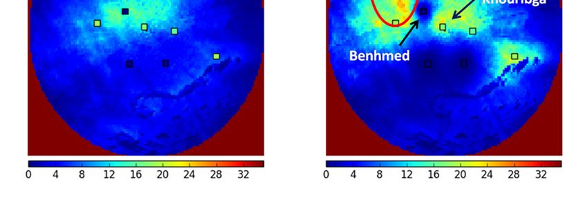
Hydrology 2019, 6, 41                                                                                4 of 13

2.1.3. The Relationship between Rainfall Rate and Radar Reflectivity
     Weather radars indirectly measure the precipitation amount on the ground. In fact, they measure
the power of the electromagnetic signal backscattered by raindrops to the radar antenna. This power is
expressed as in Equation (1):
                                                    C
                                              Pr = 2 Z                                            (1)
                                                    r
where Pr [W] is the received power, r [m] is the range from the radar, C [Wm5 mm−6 ] is the radar
constant and Z [mm6 m−3 ] is the reflectivity.
     Both the radar reflectivity and rainfall rate, R [mm h−1 ], are functions of the raindrop size
distribution (Equations (2) and (3)):
                                                 Z     Dmax
                                        Z=                    N0 e−ΛD D6 dD                             (2)
                                                   0

                                                 Dmax
                                                              πD3
                                         Z                        !
                                    R=                  N (D)       v(D)dD                              (3)
                                             0                 6
where N is raindrop distribution N (D) = N0 e−ΛD , N0 = 8000 m−3 mm−1 , Λ = 4.1 R−0.21 mm−1 , D is drop
diameter in mm and v is drop terminal velocity.
    Therefore, the relationship between Z and R is assumed to follow a power law [25], as expressed
by Equation (4):
                                              Z = a ∗ Rb                                             (4)

    The coefficients a and b depend on the raindrop size distribution. Different sets of these coefficients
were empirically calculated by former studies [26,27] according to the meteorological situation and the
hydrometeor type (e.g., rain, snow or hail).

2.2. Radar–Gauge Merging Method

2.2.1. Quality Control of Radar Reflectivity
    The tool wradlib (https://wradlib.org) was used to process data. This tool contains a number of
programs that treat radar data for hydrological and meteorological applications. The quality control
process consisted of the following steps:

•     Clutter detection and filtering: Gabella and Notarpietro [28] proposed an easy-to-implement
      method based on a two-step algorithm. The first step consists of verifying the spatial consistency
      for each pixel according to its neighborhood, due to the fact that noisy echoes usually have larger
      spatial variability compared to the precipitation field. The second step is a test of compactness
      based on the difference between clutter and rain area/perimeter characteristics. This method
      produces satisfactory results for C-band radars no matter what the weather conditions are.
•     Correction of signal attenuation: The main cause for systematic underestimation of radar rainfall
      is the attenuation of the radar signal by raindrops, especially in cases of heavy rain. The current
      study used Kraemer and Verworn’s [29] gate-by-gate approach for attenuation correction. This
      method required no additional inputs (e.g., microwave links or mountain returns) other than the
      radar reflectivity. The attenuation for the first gate was calculated using the K–Z relationship
      (Equation (5)):
                                                   K0 = α ∗ Zβ                                        (5)

     The attenuation K0 was then used to increase the reflectivity of the gates beyond. For a given
gate, i, Ki is calculated using the reflectivity Zi and the sum of the attenuation from previous gates
(Equation (6)):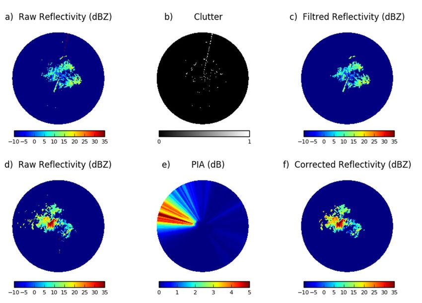
Hydrology 2019, 6, 41 5 of 13
β
i−1
X
Ki = α ∗ Zi + K j ∗ 2∆r (6)
j=0
where ∆r = 1 km is the gate length, and coefficients α and β are calculated in real time.
First, the “initial guess” values of 1.67 × 10⁻⁴ and 0.7 were given to α and β, respectively, which
generally produced an overestimation of the attenuation [29]. Then, an iterative algorithm was
applied to calculate the optimum α and β. This method was efficient and did not require any further
independent reference for α and β calculation.
• Z-R conversion: Due to a lack of information about the hydrometeor’s type and the raindrop size
distribution of Khouribga City’s radar, multiple combinations of a and b were tested, especially
those used for the U.S. Weather Surveillance Radar 1988 Doppler (WSR-88D) [30]. The comparison
with rain gauges showed that the values a = 75 and b = 2 were the most reliable coefficients for
the studied rainfall events.
2.2.2. Gauge Adjustment Model
The gauge adjustment performed in the current study used a mixed error model [31]. This model
assumes that the error (Rgauge − Rradar ) has mainly multiplicative (δ) contributions for large errors. The
additive term ε is used in case of a small difference between the radar and the gauge (Equation (7)):
R gauge − Rradar = δ ∗ Rradar + ε (7)
The technical implementation is based on a least squares estimation of δ and ε for each rain gauge
location by minimizing the sum(δ2 + ε2 ). Therefore, the formulation of δ and ε [32] is as follows
(Equations (8) and (9)):
R gauge − Rradar
ε= (8)
R2radar + 1
R gauge − ε
δ= −1 (9)
Rradar
Using an inverse distance weighting, the coefficients ε and δ are then interpolated to the other
pixels (Equations (10) and (11)):
PN 1
i=1 d δi
δp = PN i (10)
1
i=1 d i
PN
i=1 d i εi
1
εp = PN (11)
1
i=1 d i
where di is the distance between the radar pixel p and the ith rain gauge, while N is the number of
rain gauges.
Finally, at the pth pixel, the adjusted radar QPE is given by Equation (12):
Radj = 1 + δp ∗ Rradar + εp (12)
3. Results and Discussion
In order to assess the impact of the proposed radar–gauge merging method, a study of 10 winter
stratiform precipitation events over November and December 2016 and January 2017 was performed.
The meteorological situation was usually characterized by north-to-northwest perturbations, generating
light-to-moderate stratiform precipitations over the Moroccan Atlantic coast and plains, in the west of
the Atlas Mountains. The maximum observed precipitation amounts for the studied events varied
between 10 mm and 35 mm.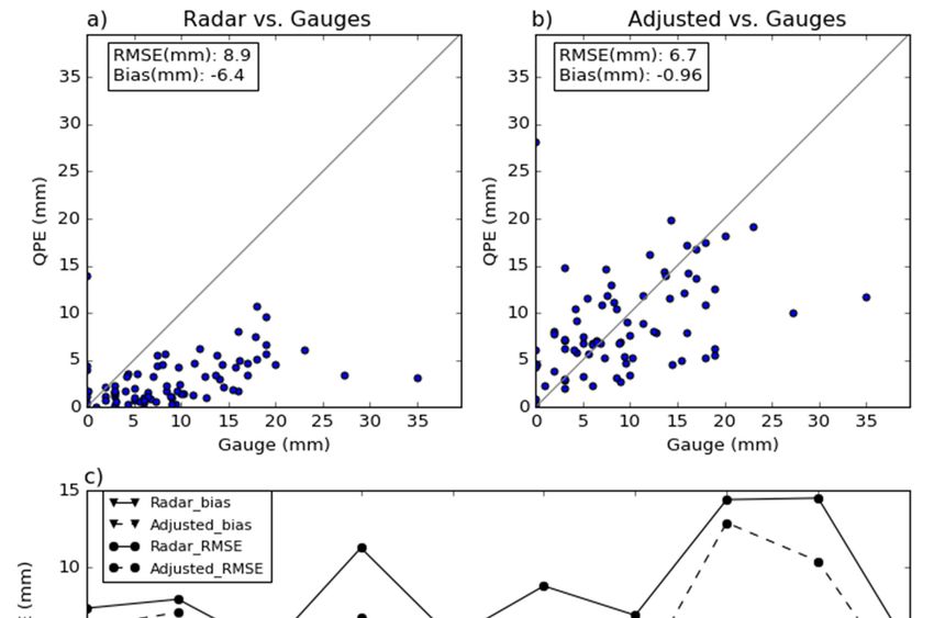
Hydrology 2019, 6, 41                                                                                           6 of 13

3.1. Assessment of Quality Control
     The Khouribga City radar gives reflectivity at 10 elevation angles every 10 min. A quality
control was applied to the reflectivity from each elevation angle and at each time step. As explained
in the methodology section, it consisted of clutter elimination and signal attenuation correction.
The reflectivity was then converted to a rainfall rate using the Z–R relationship. The 10-min
deduced rainfall depths were integrated to produce a cumulated rainfall over 24 h. The resulting
three-dimensional (3D) field employed polar coordinates. Therefore, geo-referencing was needed to
project this 3D field onto the UTM (Universal Transverse Mercator) system. Then, the inverse distance
weighting method was applied in order to interpolate the data on a regular grid with 2.5 km horizontal
resolution and 250 m vertical resolution. Over the study area, the surface altitude varied considerably
between the northwest coastal zone, characterized by its lower altitude, and the mountainous region at
the southeast. The use of a lower Constant Altitude Plan Position Indicator (CAPPI) would increase the
masked area, while the use of a higher CAPPI might worsen the overshooting problem. Consequently,
instead of using radar CAPPI at a fixed level, a MAXI-CAPPI was produced. This could be achieved by
projecting the vertical maximum of the 3D cumulated rainfall field in a horizontal plane (considered as
radar-only QPE).
     The radar reflectivity at elevation angle 0◦ for December 16, 2016 at 08:30 UTC is presented in
Figure 2a. It indicates contamination with clutter, which took the form of a spoke in the north of the
radar area. This problem is typically due to WIFI interference, as is the case for long-distance radio
telecommunications, wherein WIFI instruments emit waves at a similar frequency to the C-band radar.
This interference is very harmful for radar rainfall estimation [33]. The Gabella filter was used
 Hydrology 2019, 6, x FOR PEER REVIEW
                                                                                                      to
                                                                                                  7 of 14
identify and remove WIFI clutter, as shown in Figure 2b,c.

      Figure 2. (a) Raw, (b) cluttered and (c) filtered reflectivity pertaining to December 16, 2016 at 08:30 UTC;
       Figure 2. (a) Raw, (b) cluttered and (c) filtered reflectivity pertaining to December 16, 2016 at 08:30
      (d) raw, (e) path-integrated attenuation (PIA) and (f) corrected reflectivity pertaining to December 17,
       UTC; (d) raw, (e) path-integrated attenuation (PIA) and (f) corrected reflectivity pertaining to
      2016 at 02:20 UTC.
       December 17, 2016 at 02:20 UTC.
     The effectiveness of Kraemer’s attenuation correction methodology may be observed in the
      Based on
visualisation of raw  reflectivity
                 the radar’s       with noplan
                              reflectivity  clutter elimination
                                                position        or (PPI)
                                                         indicator attenuation  correction,
                                                                         at an elevation    Figure
                                                                                         angle of 0◦3a shows
                                                                                                     and the
 the 24  h cumulated    precipitations   from  December   16, 2016  at 06:00 UTC   to December    17,
corresponding path-integrated attenuation (PIA) of December 17, 2016 at 02:20 UTC. Figure 2d depicts  2016 at
 06:00 UTC. The clutter caused by WIFI interference creates two spokes of unrealistic (maximum of
 120 mm) precipitation structures in the north of the radar area. After applying the Gabella filter, this
 clutter was eliminated, as illustrated in Figure 3b.
      Although the attenuation correction strengthened the precipitation cells locally (near the radar),
 as shown in Figure 3, there was no substantial correction for the areas in the northeast sector, where
 rain gauges reached an amount of 35 mm at Rabat City (130 km distant from the radar). This was
December 17, 2016 at 02:20 UTC.
Based on raw reflectivity with no clutter elimination or attenuation correction, Figure 3a shows
the 24 h cumulated precipitations from December 16, 2016 at 06:00 UTC to December 17, 2016 at
06:00 UTC. The clutter caused by WIFI interference creates two spokes of unrealistic (maximum of
Hydrology
120 mm)2019, 6, 41
precipitation structures in the north of the radar area. After applying the Gabella filter,7 of 13
this
clutter was eliminated, as illustrated in Figure 3b.
a cellAlthough the attenuation
core of reflectivity correction
with values strengthened
up to 35 dBZ locatedthe nearprecipitation
the radar. Acells locallyof
correction (near the
up to radar),
5 dB was
as shown in Figure 3, there was no substantial correction for the areas in the northeast sector,
performed in the west sector of the radar (Figure 2e) and the corrected reflectivity is shown in Figure where
2f.
rain gauges reached an amount of 35 mm at Rabat City (130 km distant from the radar).
Based on raw reflectivity with no clutter elimination or attenuation correction, Figure 3a shows This was
probably
the due to the
24 h cumulated small amount
precipitations fromof precipitation
December near
16, 2016 the radar.
at 06:00 UTC toConsidering
December 17, the stratiform
2016 at 06:00
precipitations studied were mainly generated at low altitude, underestimation of
UTC. The clutter caused by WIFI interference creates two spokes of unrealistic (maximum of 120 mm)precipitation by
the radar QPE could be due to overshooting or partial filling of the radar beam [34]. In addition, the
precipitation structures in the north of the radar area. After applying the Gabella filter, this clutter was
beam width is about 2 km at 130 km, which can reduce the reflectivity detected in the scan volume
eliminated, as illustrated in Figure 3b.
and consequently cause underestimation.
Figure
Figure 3. (a)Raw
3.(a) Rawand
and(b)
(b)corrected
corrected radar
radar quantitative
quantitative precipitation
precipitation estimation
estimation (QPE)
(QPE) from
from December
December
16, 2016 at 06:00 UTC to December 17, 2016 at 06:00 UTC.
16, 2016 at 06:00 UTC to December 17, 2016 at 06:00 UTC.
Although the attenuation correction strengthened the precipitation cells locally (near the radar), as
shown in Figure 3, there was no substantial correction for the areas in the northeast sector, where rain
gauges reached an amount of 35 mm at Rabat City (130 km distant from the radar). This was probably
due to the small amount of precipitation near the radar. Considering the stratiform precipitations
studied were mainly generated at low altitude, underestimation of precipitation by the radar QPE
could be due to overshooting or partial filling of the radar beam [34]. In addition, the beam width is
about 2 km at 130 km, which can reduce the reflectivity detected in the scan volume and consequently
cause underestimation.
3.2. Validation of the Adjusted Radar Rainfall Estimate
3.2.1. General Performances
Radar-only QPEs (24 h) were firstly retrieved from the quality checked reflectivity results for the
studied events and then used in the adjustment model. For adjusting purposes, the radar rainfall
estimate should be calculated at the gauge point. As such, the nearest nine grid points to the gauge
location were selected for the radar-only QPEs. The median from this sample was considered as the
radar estimated rainfall.
The radar QPE, before and after adjustment, was compared to the rain gauge for 10 rainfall cases.
This comparison raised difficult issues; in addition to the quality of both the radar and the gauge’s
data, numerous factors had an important contribution. The gauge gave measurements of the surface
precipitation over an area of about 200 cm2 , while the radar estimated the mean precipitation amount
of the upper levels of the atmosphere over a 6.25 km2 pixel. Other factors could also be taken into
account, such as the precipitation structures, the terrain specifications and the wind-drift effect.
The study area was covered by 24 h cumulated precipitations provided by 11 rain gauges. The
gauge network was used for adjustment with no available additional gauge data for independent
validation. Assessment of the quality of the adjusted QPE was performed using a cross-validation. For
each event, a “leave-one-out” approach was applied, which meant that one rain gauge was considered
as the test case and removed while the adjustment was performed using the remaining gauges. TheHydrology 2019, 6, 41 8 of 13
adjusted QPE was then evaluated on the removed gauge. This procedure was repeated for each of the
available gauges.
To quantify the estimation error, the root mean square error (RMSE, Equation (13)) and the bias
(Equation (14)) were calculated as follows,
q 2
PN
i=1 Rradar − R gauge
RMSE = (13)
N
PN
i=1 (Rradar − R gauge )
Bias = (14)
N
Figure 4 shows the scatter plots of the dispersion of 24 h radar-only QPE (Figure 4a) and the
cross-validation of the adjusted QPE (Figure 4b) versus the rain gauges for all studied events. The
radar-only QPE usually underestimates the gauges with a bias of −6.4 mm (37% within a distance of
50 km) and a RMSE of 8.9 mm. The use of the radar–gauge merging method brought a substantial
improvement. In fact, the cross-validation of the adjusted QPE showed a reduction of the bias to −0.96
mm and the
Hydrology RMSE
2019, to PEER
6, x FOR 6.7 mm.
REVIEW 9 of 14
Figure (a)(a)
4. 4.
Figure Scatter
Scatterplots
plotsofof24
24hhradar-only
radar-only QPE
QPE distribution and(b)
distribution and (b)the
thecross-validation
cross-validation of of
2424
h h
adjusted
adjustedQPE
QPE versus
versusthe
thegauge
gaugeobservations
observationsfor
forall
all the
the studied rainfallevents.
studied rainfall events.(c)
(c)Statistics
Statisticsinin term
term of of
bias (triangle)
bias (triangle)and
androot
rootmean
meansquare
squareerror
error(RMSE)
(RMSE) (dot) of the
the radar-only
radar-onlyQPEQPEversus
versusgauges
gauges (solid)
(solid)
andand
cross-validation of the adjusted QPE (dashed) for the 10 studies
cross-validation of the adjusted QPE (dashed) for the studies cases. cases.
3.2.2. Case Study
To assess the effective impact of the adjustment method, the 8th case (held on December 16,
2016) was deeply investigated. This event was characterized by a strong RMSE (14.4 mm) and a bias
of –8.3 mm. The 24 h rainfall amounts measured by the rain gauges (Rgauge), as well as the radar-only
QPE (Rradar), are shown in Table 2.Hydrology 2019, 6, 41 9 of 13
Case-by-case error statistics (bias and RMSE) for cross-validation of the radar-only QPE and the
adjusted QPE are presented in Figure 4c. Accordingly, the bias was considerably reduced for all the
studied cases. There was also a RMSE improvement for almost all the cases. The enhancement was
clear for cases with large errors, such as in 4, 6, 8 and 9. In fact, these events were characterized by an
important precipitation amount, especially for gauges more than 100 km from the radar.
3.2.2. Case Study
To assess the effective impact of the adjustment method, the 8th case (held on December 16, 2016)
was deeply investigated. This event was characterized by a strong RMSE (14.4 mm) and a bias of −8.3
mm. The 24 h rainfall amounts measured by the rain gauges (Rgauge ), as well as the radar-only QPE
(Rradar ), are shown in Table 2.
Table 2. Rain gauge measurements, 24 h radar-only QPE and adjusted QPE cross-validation at different
gauge locations for December 16, 2016.
Gauge Location Distance from Radar-only Adjusted QPE
Gauge (mm)
(Cities) Radar (km) QPE (mm) Cross-Validation (mm)
Khouribga 2.5 18 10.7 5.2
Casablanca 104 18 5 17.5
Mohammedia 105 20 4.5 18.2
Nouasseur 82 23 6.1 19.1
Rabat 134 35 3.2 11.7
Settat 63 19 9.6 12.6
Ouad Zem 68 16 8 7.9
Benhmed 36 0 14 28.2
Elbrouj 44 0 3.9 4.2
Ksiba 104 19 6.6 6.2
Fquih Ben Salah 44 0 4.4 6.1
The radar-only QPE generally underestimated the rainfall detected by the rain gauges. The
distance from the radar increased the underestimation—most notably in the case of Rabat City, located
134 km from the radar. The cross-validation of the adjusted QPE is also reported in Table 2. The 24 h
adjusted QPE (Figure 4d) fits the gauge data more than the 24 h radar-only QPE data (Figure 4c).
Indeed, this improvement was specifically remarked upon for the northwest sector of the radar, which
was covered by homogeneous precipitations. However, for some gauges, the cross-validation of the
adjusted QPE did not reveal a positive impact; for example, in Khouribga and Benhmed cities. This
finding was essentially due to the discontinuous aspect of the precipitation field and the impact of the
surrounding gauges.
An independent validation was required to evaluate the relative performance of the proposed
radar–gauge merging method. This validation was performed, taking as reference the African Rainfall
Climatology version 2 (ARC2) 24 h cumulated precipitations produced by the Climate Prediction
Centre (CPC) of the U.S. National Oceanic and Atmospheric Administration (NOAA).
As described by Novella and Thiaw [35], ARC2 daily precipitation analysis is based on several
input sources, specifically rain gauges and geostationary satellite data. Daily binary and graphical
output files are produced with a resolution of 0.1◦ , covering Africa from 40◦ south to 40◦ north and
from 20◦ west to 55◦ east. Validation with independent gauge data shows that the ARC2 precipitations
have an efficient quality and can be used to characterize rainfall events over Africa.
For the studied event, unlike the automatic weather stations, the rain data from synoptic stations
were included in the ARC2 precipitations.
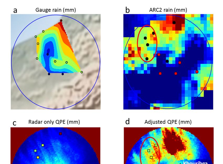
Figure 5 presents the validation of the precipitation field regarding the ARC2 data, and shows
that the field produced by a linear interpolation of the gauge data (Figure 5a) gave local information,
but was unable to reproduce the precipitation structure over a larger area. The radar-only QPEHydrology 2019, 6, 41 10 of 13
(Figure 5c) strongly underestimated the rainfall amounts. As for the adjusted rainfall field (Figure 5d),
it generally matched the ARC2 data (Figure 5b). In fact, spatial structures and precipitation amounts
were improved after adjustment. The adjustment helped to reproduce precipitation cells of more than
20 mm that were present in the ARC2 product (red ellipses in Figure 5b,d). The adjustment was also
useful in strengthening the precipitation amounts, especially in the north of the radar area. Thanks to
its high resolution (2.5 km against 10 km for ARC2), the adjusted QPE showed small-scale structures
that could not be identified in the ARC2 rain field. However, an overestimation was observed due
to the 35 mm rain gauge (Rabat City) and the lack of other surrounding rain gauges. At first glance,
the 0 mm observed in Benhmed appeared to be unrealistic. However, the 0 value is coherent with the
ARC2 field (Figure 5b) that did not include this rain gauge in its analysis. The overestimation11byofthe
Hydrology 2019, 6, x FOR PEER REVIEW 14
radar QPE was probably due to the use of MAXI-CAPPI.
Figure 5. 24 h cumulated precipitations (mm) from December 16, 2016 at 06:00 UTC to December 17,
2016 at 06:00 UTC. (a) Interpolation of the rain gauges, and (b) African Rainfall Climatology version 2
Figure
(ARC2)5.daily
24 h cumulated precipitations
precipitation. (mm) from
The black circles December
are synoptic 16, 2016
stations at 06:00
while UTC
the red to December
ones 17,
are automatic
2016 at 06:00 UTC. (a) Interpolation of the rain gauges, and (b) African Rainfall Climatology
weather stations. (c) Radar-only QPE, and (d) adjusted QPE. The squares represent the rain gauges version 2
(ARC2)
locationdaily precipitation.
colored according to The
theblack circles
observed are synoptic
precipitation stations while the red ones are automatic
amount.
weather stations. (c) Radar-only QPE, and (d) adjusted QPE. The squares represent the rain gauges
The southeast
location sector of to
colored according the
theradar wasprecipitation
observed masked by amount.
the Atlas Mountains, which created a beam
blockage and prevented a satisfactory detection of the precipitation over this area. The merging
4. Discussion and Conclusions
The current study aimed to improve the rainfall estimation based on Moroccan weather radars.
By applying the Gabella filter, the quality control methodology was able to eliminate WIFI and
ground clutter. However, the study of rainfall events over November-December 2016 and in January
2017 showed an underestimation of the radar-only QPE according to the rain gauges. TheHydrology 2019, 6, 41 11 of 13
method was unable to deal with such phenomena, especially with the dearth of gauge observations
over the mountains.
4. Discussion and Conclusions
The current study aimed to improve the rainfall estimation based on Moroccan weather radars.
By applying the Gabella filter, the quality control methodology was able to eliminate WIFI and ground
clutter. However, the study of rainfall events over November-December 2016 and in January 2017
showed an underestimation of the radar-only QPE according to the rain gauges. The attenuation
correction alone was unable to sufficiently strengthen the precipitation cells far from the radar
(>100 km) since, in all studied cases, there were only light to moderate precipitations near the radar.
The underestimation was probably due to an overshooting problem of winter stratiform precipitations,
mainly generated at low altitude.
The adjustment based on a mixed model produced improved radar QPE, as shown by the
cross-validation of the adjusted QPE versus gauges. The detailed study of the events of December 16,
2016 showed the positive impact of the gauge adjustment and also the sensitivity of the results to the
density of the gauge network.
A comparison with ARC2 precipitation analysis revealed that the adjustment method had a
positive impact on the precipitation structure and intensity. Indeed, the precipitation cells generally
fitted the ARC2 field, especially in the northwest sector, despite an overestimation found near Rabat
City due to the lack of surrounding gauges. These findings agree with former studies in similar
conditions [4], which also showed a better quality and a relevance of the hydrological applications of
adjusted rainfall radars when compared to rain gauges, raw radars or satellites precipitation estimations.
These promising results may certainly be enhanced by the use of a high density gauge network,
especially for spatially-discontinuous rainfall events. More case studies should be performed to
thoroughly investigate the impact of different hydrometeor types, such as snow or hail, associated with
snowfall or orographic precipitations over the Atlas Mountains. In addition, the use of further data
sources like satellites and NWP analysis will doubtlessly bring more accuracy to the adjusted QPE. When
it comes to a rough terrain like the study area, merging methods [4] or using orographic precipitation
climatology [36] should be tested in order to improve the radar rainfall products, particularly when
the constraints are specifically related to the orography.
Author Contributions: Investigation, Z.S.; Methodology, Z.S.; Supervision, S.M.; Validation, Z.S. and S.M.;
Writing—original draft, Z.S.; Writing—review & editing, S.M.
Funding: This research received no external funding.
Acknowledgments: The authors are grateful to the reviewers for their comments and suggestions improving the
manuscript. The authors also thank Siham Sbii, Fatima-Zahra Hdidou, Khalid Elrhaz, Driss Bari and Mohammed
Nabahani for the useful discussions of this work and for their help in revising the manuscript.
Conflicts of Interest: The authors declare no conflict of interest.
References
1. Germann, U.; Berenguer, M.; Sempere-Torres, D.; Zappa, M. REAL—Ensemble radar precipitation estimation
for hydrology in a mountainous region. Q. J. R. Meteorol. Soc. 2009, 135, 445–456. [CrossRef]
2. Harrison, D.L.; Norman, K.; Pierce, C.; Gaussiat, N. Radar products for hydrological applications in the UK.
Proc. ICE Water Manag. 2012, 165, 89–103. [CrossRef]
3. Liu, J.; Bray, M.; Han, D. A study on WRF radar data assimilation for hydrological rainfall prediction.
Hydrol. Earth Syst. Sci. 2013, 17, 3095–3110. [CrossRef]
4. Gilewski, P.; Nawalany, M. Inter-Comparison of Rain-Gauge, Radar, and Satellite (IMERG GPM) Precipitation
Estimates Performance for Rainfall-Runoff Modeling in a Mountainous Catchment in Poland. Water 2018, 10,
1665. [CrossRef]
5. Sokol, Z. Assimilation of extrapolated radar reflectivity into a NWP model and its impact on a precipitation
forecast at high resolution. Atmos. Res. 2010, 100, 201–212. [CrossRef]Hydrology 2019, 6, 41 12 of 13
6. Wattrelot, E.; Caumont, O.; Mahfouf, J.F. Operational Implementation of the 1D+3D-Var Assimilation Method
of Radar Reflectivity Data in the AROME Model. Mon. Weather Rev. 2014, 142, 1852–1873. [CrossRef]
7. Maiello, I.; Ferretti1, R.; Gentile, S.; Montopoli, M.; Picciotti, E.; Marzano, F.S.; Faccani, C. Impact of radar data
assimilation for the simulation of a heavy rainfall case in central Italy using WRF-3DVAR. Atmos. Meas. Tech.
2014, 7, 2919–2935. [CrossRef]
8. Lopez, P.; Bauer, P. 1D + 4D-Var assimilation of NCEP stage IV radar and gauge hourly precipitation data at
ECMWF. Mon. Weather Rev. 2007, 135, 2506–2524. [CrossRef]
9. Lopez, P. Direct 4D-Var Assimilation of NCEP Stage IV Radar and Gauge Precipitation Data at ECMWF.
Mon. Weather Rev. 2011, 139, 2098–2115. [CrossRef]
10. Lien, G.Y.; Kalnay, E.; Miyoshi, T. Effective assimilation of global precipitation: Simulation experiments.
Tellus A Dyn. Meteorol. Oceanogr. 2013, 65. [CrossRef]
11. Ban, J.; Liu, Z.; Zhang, X.; Huang, X.Y.; Wang, H. Precipitation data assimilation in WRFDA 4D-Var:
Implementation and application to convection-permitting forecasts over United States. Tellus A Dyn. Meteorol.
Oceanogr. 2017, 69. [CrossRef]
12. Hunter, S. WSR-88D Radar Rainfall Estimation: Capabilities, Limitations and Potential Improvements.
Natl. Weather Dig. 1996, 20, 26–38.
13. Villarini, G.; Krajewski, W.F. Review of the different sources of uncertainty in single polarization radar-based
estimates of rainfall. Surv. Geophys. 2010, 31, 107–129. [CrossRef]
14. Berne, A.; Krajewski, W.F. Radar for hydrology: Unfulfilled promise or unrecognized potential?
Adv. Water Resour. 2013, 51, 357–366. [CrossRef]
15. Faure, D.; Auchet, P.; Engasser, E. Attenuation caused by direct rainfall on a C band radar: 1998 campaign
of measurements in Nancy. In Proceedings of the 3th International Workshop on Rainfall in Urban Areas,
Pontresina, Switzerland, 10–13 December 2000; pp. 171–176.
16. Harrison, D.L.; Driscoll, S.J.; Kitchen, M. Improving precipitation estimates from weather radar using quality
control and correction techniques. Meteorol. Appl. 2000, 6, 135–144. [CrossRef]
17. Delrieu, G.; Wijbrans, A.; Boudevillain, B.; Faure, D.; Bonnifait, L.; Kirstetter, P.E. Geostatistical radar-rain
gauge merging: A novel method for the quantification of rain estimation accuracy. Adv. Water Resour. 2014,
71, 110–124. [CrossRef]
18. Jewell, S.A.; Gaussiat, N. An Assessment of Kriging Based Rain-Gauge—Radar Merging Techniques. Q. J. R.
Meteorol. Soc. 2015, 141, 2300–2313. [CrossRef]
19. Goudenhoofdt, E.; Delobbe, L. Evaluation of radar-gauge merging methods for quantitative precipitation
estimates. Hydrol. Earth Syst. Sci. 2009, 13, 195–203. [CrossRef]
20. Tabary, P. The new French radar rainfall product. Part I: Methodology. Weather Forecast. 2007, 22, 393–408.
[CrossRef]
21. Tabary, P.; Desplats, J.; Do Khac, K.; Eideliman, F.; Gueguen, C.; Heinrich, J.-C. The new French radar rainfall
product. Part II: Validation. Weather Forecast. 2007, 22, 409–427. [CrossRef]
22. Zhang, J.; Howard, K.; Langston, C.; Vasiloff, S.; Kaney, B.; Arthur, A.; Van Cooten, S.; Kelleher, K.;
Kitzmiller, D.; Ding, F.; et al. National Mosaic and Multi-sensor QPE (NMQ) System: Description, Results,
and Future Plans. Bull. Amer. Meteor. Soc. 2011, 92, 1321–1338. [CrossRef]
23. Malkomes, M. The Morocco Weather Radar Network mix of upgraded radars and new ones-A success
story. In Proceedings of the 8th Eutopean Conference on Radar in Meteorology and Hydrology,
Garmisch-Partenkirchen, Germany, 1–5 September 2014.
24. Salek, M.; Novak, D. Operational application of combined radar and rain gauges precipitation estimation at
the CHMI. In Proceedings of the 3th European Conference on Radar in Meteorology, Visby, Sweden, 6–10
September 2004; ERAD Publication Series 2. pp. 16–20.
25. Marshall, J.S.; Palmer, W.M. The distribution of raindrop with size. J. Meteorol. 1948, 5, 165–166. [CrossRef]
26. Chapon, B.; Delrieu, G.; Gosset, M.; Boudevillain, B. Variability of raindrop size distribution and its effect on
the Z–R relationship: A case study for intense Mediterranean rainfall. Atmos. Res. 2008, 87, 52–65. [CrossRef]
27. Uijlenhoet, R. Raindrop size distributions and radar reflectivity–rain rate relationships for radar hydrology.
Hydrol. Earth Syst. Sci. 2001, 5, 615–628. [CrossRef]
28. Gabella, M.; Notarpietro, E. Ground clutter characterization and elimination in mountainous terrain.
In Proceedings of the 2nd European Conference on Radar in Meteorology and Hydrology, Delft,
The Netherlands, 18–22 November 2002; pp. 303–311.Hydrology 2019, 6, 41 13 of 13
29. Kraemer, S.; Verworn, H.R. Improved C-band radar data processing for real time control of urban drainage
systems. In Proceedings of the 11th International Conference on Urban Drainage, Edinburgh, Scotland, UK,
31 August–5 September 2008.
30. Chilson, P.B. “Z-R relationships”, Weather Radar Applications ECE/METR 5683. 2008. Available online:
http://www.ou.edu/radar/z_r_relationships.pdf (accessed on 23 May 2019).
31. Heistermann, M.; Jacobi, S.; Pfaff, T. Technical Note: An open source library for processing weather radar
data (wradlib). Hydrol. Earth Syst. Sci. 2013, 17, 863–871. [CrossRef]
32. Pfaff, T. Radargestuetzte Schaetzung von Niederschlagsensembles. Operationelle Abfluss-und
Hochwasservorhersage in Quellgebieten. Final Project Report. University of Stuttgart: Stuttgart, Germany;
pp. 113–118. Available online: http://www.rimax-hochwasser.de/fileadmin/user_uploads/RIMAX_PUB_22_
0015_Abschlussbericht%20OPAQUE_final.pdf (accessed on 23 July 2018). (In German).
33. Scovell, R.; Gaussiat, N.; Matthews, M. Recent Improvements to the Quality Control of Radar Data for
the OPERA Data Centre. In Proceedings of the 36th radar conference of American Meteorological Society,
Breckenridge, CO, USA, 16–20 September 2013.
34. Delobbe, L. Estimation des Précipitations à L’aide d’un Radar Météorologique; Scientific and technical publication.
Nr 44; Royal Meteorological Institute of Belgium: Brussels, Belgium, 2006. (In French)
35. Novella, N.S.; Thiaw, W.M. African rainfall climatology version 2 for famine early warning systems. J. Appl.
Meteor. Climatol. 2013, 52, 588–606. [CrossRef]
36. Zhang, J.; Qi, Y.; Langston, C.; Kaney, B.; Howard, K. A real-time algorithm for merging radar QPEs with
rain gauge observations and orographic precipitation climatology. J. Hydrometeorol. 2014, 15, 1794–1809.
[CrossRef]
© 2019 by the authors. Licensee MDPI, Basel, Switzerland. This article is an open access
article distributed under the terms and conditions of the Creative Commons Attribution
(CC BY) license (http://creativecommons.org/licenses/by/4.0/).You can also read