Dynamic range improvement for some Canon dSLRs by alternating ISO during sensor readout
←
→
Page content transcription
If your browser does not render page correctly, please read the page content below
Dynamic range improvement for some∗ Canon dSLRs
by alternating ISO during sensor readout
a1ex
July 16, 2013
Would you trade half of vertical resolution for 3 stops of extra dynamic range?
If you are tempted to answer “yes”, read on.
1 Introduction
If you are lurking on popular photo forums, you have probably noticed that some people say
Nikon/Sony/Pentax/others have more dynamic range than Canon cameras [1, 2, 3]. The differ-
ence is visible in extreme lighting conditions - when you try to bring shadow detail, the image
from Canon dSLRs tends to get a bit noisier (Figure 1).
Can we do something about it?
YES.
It’s all about how you are scanning the sensor.
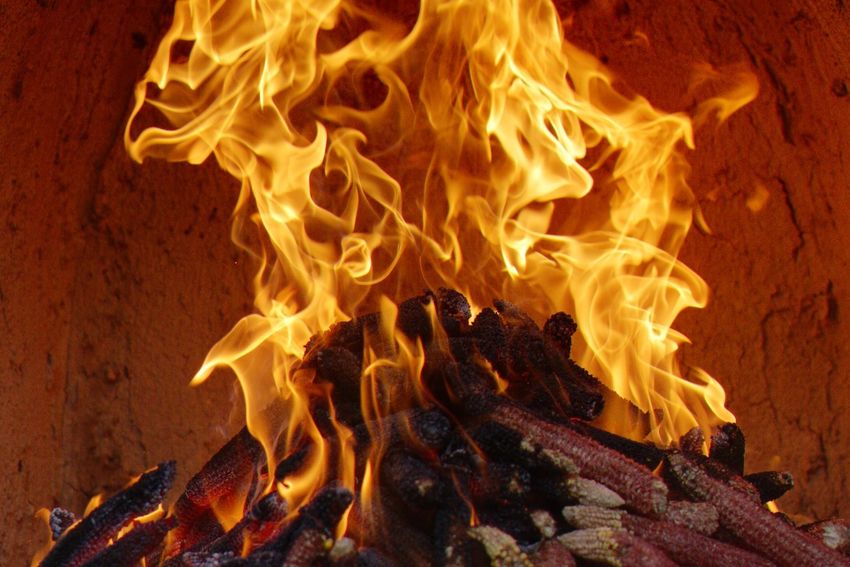
Figure 1: 5D3 vs D800 shadow recovery: ISO 100, f/8, 1/2000, +4EV in post.
Credits: Julian Huijbregts, www.digifotopro.nl
∗ At the time of writing, only 5D Mark III and 7D are known to work. See What about other cameras? on page 5.
1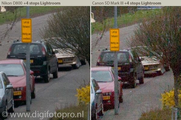
With Nikon/Sony/Pentax sensors, you get little or no improvement in shadows if you are
shooting at ISO 800, or if you are shooting at ISO 100 and applying a +3 exposure compen-
sation in post. Some people call these sensors ISO-less [4].
With Canon sensors, when you shoot at ISO 100 the image looks quite clean, but once you start
boosting the shadows (applying positive exposure compensation in post), you get a lot of noise.
You get much better results if you shoot at a higher ISO from the beginning (of course, with
identical shutter, aperture and lighting conditions), but you lose dynamic range and you may
have to clip some highlights.
In particular, with the 5D Mark III, at ISO 100 you get 10.97 stops of dynamic range, and at
ISO 1600 you get 9.94 stops according to DxO [5]. When raising the ISO from 100 to 1600, you
are shifting the dynamic range towards the shadows by 4 stops and shortening it by 1 stop. In
other words, you throw away 4 stops of highlight data (they get clipped), and you get in return
3 stops of shadow detail.
This technique is very similar to the “zero noise” “technique of the 4 f-stops“ developed by
Guillermo Luijk [6], where he uses only two bracketed images, at 0 and +4 EV, to achieve great
interior shots without the ”radioactive“ HDR look. Emil Martinec gives a hint on how to shoot
at ISO 100 and 1600 simultaneously [7], but this requires two separate amplifiers fed from the
same sensor data. We’ll get around it with a simple software trick and a little math.
Yes, all this smells a bit like HDR, which proved extremely popular when it was introduced
in Magic Lantern back then in December 2011 [8]. But traditional HDR has a disadvantage of
requiring two or more exposures, which makes it unsuitable for moving subjects. To address
this issue, Soviet Montage used two Canon 5D Mark II cameras and a beam splitter [9]. Fuji
designed a sensor that uses a similar technique, where half of the pixels are optimized for high-
lights and half for shadows (SuperCCD SR series) [10, 11].
Also RED developed the HDRxTM method for Epic and Scarlet cameras, which uses two dif-
ferent exposure times. The primary exposure is normal, and uses the standard aperture and
shutter settings (the “A frame”). The secondary exposure is typically for highlight protection,
and uses an adjustable shutter speed that is 2-6 stops faster (the “X frame”) [12]. However,
the different shutter speeds may result in motion artifacts, but the two images are overlapping
properly (sure, with different amounts of motion blur), therefore RED considers it a creative
tool (scroll down to ”Controlling motion blur“ in [12]).

2    Canon’s uncompressed 14-bit raw format
The compressed raw format is already covered in [13] and implemented in open-source raw
converters, so it goes beyond the scope of this document. We’ll focus on the uncompressed
14-bit data found in Canon’s image buffers from the camera itself.
This format is used by Canon code when saving still photos, and it is codenamed MEM1 in the
firmware; some relevant strings are sdsMem1ToRawCompression and sdsMem1ToJpegDevelop. It
can be enabled in LiveView, at lower resolution, with a debug flag called lv save raw, present
in all past and current Canon dSLRs starting with 40D.
The format was guessed by trial and error: first we have guessed the image size, in bytes, by
applying FFT to the data stream and examining the peaks, then we have guessed how many
pixels should be there, how many bits, and which of them are the most significant ones. CHDK

                                               2
already decoded similar 10 and 12-bit raw streams, and the format is quite similar, so we could
reuse their code for saving DNG files.
A raw image buffer is a contiguous memory region containing 14-bit pixels, where every 8
pixels are grouped in 14 bytes. Each line contains a multiple of 8 pixels (you can’t split a line
in the middle of a pixel group). To address the pixel at ( x, y), you have to know at least the
image width (pitch = width in bytes [14]), so you can select the pixel group at memory offset
(y · pitch + b x/8c · 14), and inside the group, the individual pixel is selected by ( x mod 8).
A 8-pixel group can be described in C with the following data structure:
struct raw_pixblock
{
    unsigned int b_hi: 2;
    unsigned int a: 14;         // even lines: red; odd lines: green
    unsigned int c_hi: 4;
    unsigned int b_lo: 12;
    unsigned int d_hi: 6;
    unsigned int c_lo: 10;
    unsigned int e_hi: 8;
    unsigned int d_lo: 8;
    unsigned int f_hi: 10;
    unsigned int e_lo: 6;
    unsigned int g_hi: 12;
    unsigned int f_lo: 4;
    unsigned int h: 14;         // even lines: green; odd lines: blue
    unsigned int g_lo: 2;
} __attribute__((packed));

where the structure packing order is the GCC one. If you use mingw, don’t forget to use
-mno-ms-bitfields when working with raw data.
The image data is a RGGB Bayer pattern, arranged like this:
   ab cd   ef   gh   ab   cd   ...
   RG RG   RG   RG   RG   RG   ...
   GB GB   GB   GB   GB   GB   ...
   RG RG   RG   RG   RG   RG   ...
   GB GB   GB   GB   GB   GB   ...
   ...

Raw values range from some black level to some white level (usual values are 2048 and 15000)
and they are linear. To convert them in stops (EV), subtract the black level and apply log2 :

                                         ev = log2 (max(raw − black, 1))                      (1)

where ev will be a value between 0 and almost 14. To convert from ev back to raw values:

                                                 raw = 2ev + black                            (2)

with some extra care to avoid going outside the [black...white] interval.
The raw image usually contains two black bars, at top and left side, which do not contain image
data, but can be used to estimate the black level and to analyze the noise. For example, you can
compute the standard deviation of the noise from the black area, and knowing the white and
black levels, you can approximate the dynamic range of the sensor for current settings:

                               dr = log2 (white − black mean) − log2 (black stdev)            (3)

The results should be pretty close to DxO numbers. You may get slightly different results if you
change shutter speed too, not just ISO.
                                                           3
3    ADTG/CMOS register tweaking
The ADTG is probably the chip responsible for converting CMOS analog sensel values to a
digital data stream and control its clock and address lines. It also seems to be an accurate
timing generator for this purpose [15].
The ADTG and CMOS registers are used for configuring low-level sensor timings and proba-
bly other parameters, like ISO, number of scan lines, downsampling factors and so on. These
functions can be found in Canon firmware by looking for the following strings:
[REG] @@@@@@@@@@@@ Start ADTG
[REG] ############ Start CMOS
[REG] ############ Start CMOS16
Register values can be examined by hooking a callback function in the existing ARM ASM code,
using a breakpoint. This method was implemented by g3gg0 in the adtg log module [16].
Looking at CMOS register values while changing ISO, we have noticed that CMOS register #0
takes the following values on 5D Mark III:

                ISO    CMOS register #0                ISO   CMOS register #0
                100    0x003                          1600   0x443
                200    0x113                          3200   0x553
                400    0x223                          6400   0xDD3
                800    0x333                         12800   0xFF3

       Table 1: Values of CMOS register #0, as a function of ISO, on Canon 5D Mark III

As expected, intermediate ISOs like 160 or 250 do not cause any changes in ADTG/CMOS con-
figuration. These ISOs are obtained by applying some digital gain to the raw data acquired
at the nearest full-stop ISO, and this gain is configured from the DIGIC register 0xC0F08030
(SHAD GAIN). In LiveView, the gain is only applied to the YUV image (it does not affect the 14-bit
raw data at all), but in photo mode, the gain is burned into the raw data. Don’t ask me why.
So, back to our CMOS register #0, it looks like the LSB nibble is probably some flag, and the
other two are some sort of amplifier gains. What do you think it will happen if we change this
register to 0x403 or 0x043?
It turns out... the answer to this question is the key to some massive improvement in image
quality. The sensor will scan half of the lines at ISO 100 and the other half at 1600 (Figure 2).

             Figure 2: Sampling the image sensor at ISO 100 and 1600 interlaced.

                                                4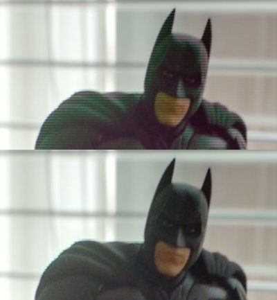
At a closer look, the ISO alternates every two lines, so the pattern looks like this: l, H, H, l, l, H,
H, l, l. You may say it would have been better to alternate every single line, right?
Well, not quite. With ISO alternating every two lines, you get complete RGGB cells at ISO 100
and complete RGGB cells at ISO 1600. With ISO alternating every single line, you would get the
RG pixels at ISO 100 and the GB pixels at ISO 1600. Good luck interpolating that ;)
Anyway. The Bayer pattern that we have now looks like this:
      ab cd ef gh          ab cd ef gh                    ab cd ef gh         ab cd ef gh

 0    RG   RG   RG   RG    RG   RG   RG   RG          0   rg   rg   rg   rg   rg   rg    rg   rg
 1    gb   gb   gb   gb    gb   gb   gb   gb          1   gb   gb   gb   gb   gb   gb    gb   gb
 2    rg   rg   rg   rg    rg   rg   rg   rg          2   RG   RG   RG   RG   RG   RG    RG   RG
 3    GB   GB   GB   GB    GB   GB   GB   GB          3   GB   GB   GB   GB   GB   GB    GB   GB
 4    RG   RG   RG   RG    RG   RG   RG   RG          4   rg   rg   rg   rg   rg   rg    rg   rg
 5    gb   gb   gb   gb    gb   gb   gb   gb          5   gb   gb   gb   gb   gb   gb    gb   gb
 6    rg   rg   rg   rg    rg   rg   rg   rg          6   RG   RG   RG   RG   RG   RG    RG   RG
 7    GB   GB   GB   GB    GB   GB   GB   GB          7   GB   GB   GB   GB   GB   GB    GB   GB
 8    RG   RG   RG   RG    RG   RG   RG   RG          8   rg   rg   rg   rg   rg   rg    rg   rg

Notice the exposure pattern may start anywhere, so we need to autodetect this when writing
the post-processing software, rather than assumming a fixed starting position.
At the risk of stating the obvious: ISO is analog amplification after sensor is read out, but before
the analog-digital conversion (ADC). It does not affect the timing in any way, so this method
will not introduce any motion artifacts.

3.1    What about other cameras?

Unfortunately, most other Canon cameras follow a different pattern for the CMOS #0 register,
without any obviously duplicate fields. As we know from Canon specs, most cameras have
a 4-channel sensor readout, except for 5D Mark III and 7D which have a 8-channel readout.
Therefore, it’s likely that our ISO trick may work on the 7D. Let’s examine the values:

                          ISO   CMOS register #0                     ISO      CMOS register #0
                          100   0b   000   000   00                  1600     0b   100   100   00
                          200   0b   001   001   00                  3200     0b   101   101   00
                          400   0b   010   010   00                  6400     0b   101   101   00
                          800   0b   011   011   00                 12800     0b   101   101   00

                 Table 2: Values of CMOS register #0, as a function of ISO, on Canon 7D

Notice the repeated pattern contains only 3 bits this time. For ISO 100/1600, we can try to set
the register to 0x80 = 0b 100 000 00, and... SUCCESS!
We can now speculate that cameras with 8-channel readout have two separate amplifier circuits,
and you can program the ISO for each one separately. We are also very sorry for the owners of
cameras with fewer channels.
The Canon 70D also has a 8-channel readout, according to [17]: ”An eight-channel read-out also
supports high speed shooting of up to seven frames per second (fps) at full resolution.“. Therefore, this
technique is likely to work on it, if we’ll be able to port Magic Lantern. Time will tell.

                                                          5
4    Separating the two exposures
Since our image contains two different exposures, the obvious way to get something useful
is to separate the dark and bright lines, obtaining two half-resolution images, which will be
combined afterwards. Of course, we need to interpolate the missing lines.
The first observation is that every missing Bayer pixel at ( x, y) has two neighbouring pixels of
the same color at ( x, y + 2) and at ( x, y − 2), therefore a straightforward interpolation method
is to average them. Don’t expect great results from this though.
For green pixels, we can make a slight improvement: the closest 3 neighbours of a green pixel
( x, y) are ( x + 1, y + 1), ( x − 1, y + 1), ( x, y − 2), or ( x + 1, y − 1), ( x − 1, y − 1), ( x, y + 2),
depending on the exact position of the pixel. Averaging these 3 neighbours should bring a little
more detail in the green channel, though I did not notice any difference.
The way averaging is performed does matter though. If the averaging is done in linear space,
where pixel values are from say 2048 to say 15500, averaging a white and a black pixel will
result in a pixel value close to 8774, which is 1 stop lower than white. When averaging black
and white, you don’t expect to get a very light gray, do you? So, it makes sense to average in
the EV domain. Figure 3 a-b shows the difference.
Another straightforward choice is to interpolate from the 6 neighbouring pixels of the same
color (3 from top, 3 from bottom). Averaging them did not improve the jagged edges; however,
taking the median of these 6 pixels seems to handle diagonal edges better (Figure 3 c).

(a) Linear averaging the closest 2-3   (b) Log averaging the closest 2-3   (c) Median of the 6 top/ bottom neigh-
neighbours (2 for R/B, 3 for G)        neighbours (2 for R/B, 3 for G)     bours (log averaging the 2 midpoints)

Figure 3: Interpolation methods. Test image: ISO 100 lines from the Batman shot, with interpo-
lation for the missing lines. Result developed in ufraw, AHD.

You should already know there are much better interpolation methods out there, starting with
the good old bicubic [18], continuing with the well-known VNG, AHD, PPG from dcraw [19],
and not forgetting the recent top-performers DCB [20] and AMaZE [21], or the less known
direction-adaptive interpolations like [22] and [23]. Of course, these algorithms are not that easy
to implement [read: I’m lazy], but if you feel like sharpening your computational photography
skills, feel free to try them and submit a patch.

                                                       6
5     Mixing the two exposures
We now have two exposures of the same scene: a dark one and a bright one. Both sub-images
are at half-resolution. We could just run them through our favorite HDR software, right?
Yes, but we can do better. We can mix the two exposures and try recover the original resolution
(or at least some of it). Megapixels are important too, right?
So, we will overlap the two exposures. Let’s consider the ISO 100/1600 example: to overlap
these two exposures, we need to darken the ISO 1600 image by 4 stops (roughly speaking), so
it looks similar to the ISO 100 one (we aim for identical midtones - Figure 4).

       Figure 4: Darkening the ISO 1600 shot (right) so it looks like the ISO 100 one (left).

Then we will combine the images as follows:
    • In highlights, we only have valid data in the ISO 100 image. The ISO 1600 one is clipped
      (by 4 stops).
    • In deep shadows, we only have valid data in the ISO 1600 image. The corresponding data
      from ISO 100 will be just noise.
    • In midtones, we have valid data at both ISOs. We can mix them and try to recover the
      resolution.
    ISO 100 :       ###...........       (11 stops)
    ISO 1600:   ####..........           (10 stops)
    Combined:   XX##..............       (14 stops)
Okay, you will say the algorithm is easy: if one is clipped, take data from the other (easy). If
one is too noisy, take data from the other (how to set the threshold?). Otherwise, discard the
interpolated data and just alternate the pixels from both images (they are identical, no?)
Well, the two exposures are not quite identical, even if we have darkened the ISO 1600 one. They
are similar, but not identical. If we assume they are identical, we will get horizontal banding
(Figure 7), but at least we can recover the full resolution in midtones.
First, the ISO 1600 image will have less noise than the ISO 100 one. So, why not just use the
ISO 1600 data everywhere, besides the top 4 stops? Because resolution matters too, and so does
aliasing and moire (which you just got because of line skipping).

                                                 7
Second, the ISO 1600 has less saturation than ISO 100. Not sure why. But you can boost the
saturation a little, and you will notice ISO 1600 remains cleaner even after that (Figure 5).
Figure 5: Midtones from ISO 100 (left) and ISO 1600 (right). Images developed with ufraw, at
+6/+2 EV to reveal the noise and saturation 1.0/1.2 to match the colors.
Third, there are some other subtle differences between these ISOs, and without knowing exactly
what’s going on behind the scenes, it’s difficult to get an accurate mathematical model.
A straightforward way is to use linear interpolation between the two images. We will use mix
factor k with values, between 0 and 1, and we’ll mix bright and dark pixel values, expressed in
EV, with bright darkened by log2 (iso hi/100) stops. The resulting image will be:
mixed = bright · (1 − k) + dark · k (4)
Therefore, k will be 0 for deep shadows, 1 for highlights and in-between values for midtones.
Knowing the approximate dynamic range at ISO 100 for Canon sensors (11 EV), and the differ-
ence between the two ISOs, the overlap will be:
iso hi
overlap = 11 EV − log2 100 (5)
The reference signal level ev is taken from the cleanest half of the image (ISO 1600 darkened):
ev = bright = bright0 − log2 iso hi
100 (6)
The smooth transition between the two exposures will start at:
iso hi
start = log2 (white − black) − overlap − log2 100 (7)
and the transition curve can be obtained easily with the cosine function (Figure 6):
π ·(ev−start)
cos overlap
, start ≤ ev ≤ start + overlap
c= 0 , ev < start (8)
1 , ev > start + overlap
1−c
k= (9)
2
Tip: you may decrease the overlap by a small amount (1 or 2 stops) to reduce shadow noise, at
the cost of lower resolution. If you do that, shift the starting point to the right by the same amount.
8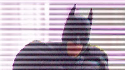
Figure 6: Mixing curves for combining bright and dark exposures with a smooth transition.

Figure 7: Comparison between mixing methods. Top: simply split and enfuse [24] the two
exposures (ISO 100/1600); Middle: smooth transition with cosine, then developed at 0 and
+4, then enfused; Bottom: full resolution (0 and +4, then enfused). Left: photo frame; Right:
video frame. Banding is much worse in the video shot because black levels were not known
accurately.

                                             9
5.1      Recovering the full resolution in midtones

As you can see from Figure 7, the result with the smooth transition is a little on the soft side (but
without any banding). The midtones created without any interpolated pixels (Figure 7, bottom)
have the same resolution as a normal picture (without dual ISO), but has some slight banding
artifacts. The banding is close to none if black level is corrected with good accuracy.
Even with perfect matching between the two images, the different noise levels in the two ISO
shots will create banding. To reduce it, we’ll try to do a smooth transition from the soft interpo-
lation to full-resolution image, based on the same cosine function from eq. (8):

                                           f = 1 − c4                                                             (10)
                                     f ullres = is bright line ? bright : dark                                    (11)
                                     output = mixed · (1 − f ) + f ullres · f                                     (12)

 Figure 8: Mixing curve for recovering full midtone resolution without (too much) banding.

      (a) soft blending with curve (9)       (b) full resolution, no blending   (c) full resolution, curves (9) and (10)

                               Figure 9: Recovering full resolution in midtones.

Why all this math? Judge yourself from Figure 9.
Notice that full-resolution recovery requires the two exposures being matched perfectly. If they
are not, you will get banding like in Figure 7, bottom right, and in this case you’ll have to live
with a softer image, obtained only with curve (9), which does not have any banding.

                                                          10
5.2 Estimating the ISO difference
The problem is easy to understand: adjust the bright image so it looks identical to the dark one,
in the overlapped areas.
In theory, this should be easy: we can assume the analog gain from ISO 1600 is exactly +4 EV,
the gain from 3200 is +5 EV and so on. So, all we have to do is to divide each ISO 1600 pixel
value by 16? Is this always true? Can we get a better estimation?
Let’s try some curve fitting.
Data set: RGGB from ISO 100 on the X axis, RGGB from ISO 1600 on Y, from the Batman shot
(Figure 10(a), green). There’s quite a bit of noise and a lot of outliers.
You might be tempted to try linear least squares, to fit a line through this data. Don’t. Linear
regression doesn’t like outliers.
If you look closer, the image noise that falls right under the clipping level will influence the
results, even if you use robust linear regression. If we want to remove the bias, we would have
to throw away a lot of useful data.
Wait. Let’s try a little trick. For every raw level on the ISO 100 image, we will compute the
median of all the corresponding pixels from the ISO 1600 image. The median will not be fooled
by the saturated pixels, unlike the mean, so unless the median itself is clipped, all these data
points are now valid and unbiased (Figure 10(a), blue).
(a) Data points, vertical mean points (biased), vertical me- (b) How important is that tiny offset? Top: line fitting
dian points (unbiased), least squares fit through medians with gain only, y = 15.70 · x; Bottom: complete line fitting,
giving ISO (slope) and black difference (constant term). y = 15.70 · ( x − 35). Full-res recovery with curves (9), (10).
Figure 10: Robust matching of dark and bright exposures
If you compare the mean and median curves, one can tell whether the median data points are
valid or not just by comparing them against white level and the noise floor. Mean points are
getting biased as the ISO 1600 image is approaching the clipping point; beyond that, there are
outliers that may be hard to detect in tricky cases.
Fitting a straight line through the median points is now an easy task, because the data set is now
clean, with most outliers removed. Notice the best fit line, y = 15.70 · ( x − 35), does not pass
through the origin, which may indicate a difference in black level in both exposures. This is
expected, because we don’t have black correction data for this particular shot. How important
is this small black difference? Figure 10(b) gives the answer.
115.3 Black level subtraction
The black level in raw image is the voltage read by the ADC in complete darkness. It looks
like that level is not zero, as you would expect for pure black, and the exact value varies with
settings, temperature and who knows what other factors.
The most obvious operation that requires correct black level is white balance. If the EXIF black
value is much lower than the real thing, you get pink cast in shadows; if it’s too high, you get
green cast. This is because white balance is usually applied by multiplying the red and blue
channels with values roughly close to 2. Obviously, this multiplication is done after subtracting
the black level from the raw data [13].
For overlapping the two exposures, black level becomes important because we have to match
them (to darken the ISO 1600 so it looks the same as ISO 100). If the black level is subtracted
correctly, all we have to do is to divide the ISO 1600 image by 16 (or, estimate the amplification
factor, which may not be exactly 16.0).
Black subtraction is essential for correcting the interference between the two ISOs, which be-
comes obvious at extreme ISO values (100/6400 or 100/12800, Figure 14). It is less important
to know the black level at ISO 100/800 or ISO 1600, where you can get great results without
bothering about black level.
The most obvious way to estimate the black level is to shoot a dark frame (take a picture with
the lens cap on), and subtract it from the raw data. Q: who does that in practice? (A: astropho-
tographers)
The raw data from Canon sensors contains two black areas at top and left sides. We don’t know
exactly how they are achieved, but [25] suggests the black region is called optical black, and these
pixels have a metal shielding in the photodiode window. Therefore, the noise pattern should be
similar to the noise from a dark frame (image taken with lens cap on). Figure 12 confirms the
theory, so we can use these black areas for noise analysis, except for the top half from the top
bar (30-40 lines out of 80, which seem to be scanned with different settings).
Dcraw computes the average for these black areas. Here’s an explanation from Dave Coffin,
found in [13]:
The best measurement of the black level is the frame of masked pixels bordering the image at
left and right. Older versions of dcraw averaged them into a single black value, while the
latest code calculates four black values according to their positions in the 2 × 2 Bayer array.
Let’s take a closer look at the noise patterns with regular ISOs (Figure 13).
The noise seems uniform and it doesn’t look like there are any differences between the 4 color
channels. Indeed, the colors are obtained through optical filters; the analog amplification is
identical, so there should be no reason to compute separate black levels for each channel.
The same noise characteristics are kept with dual ISO scanning (Figure 14). However, at extreme
settings (ISO 100/6400 and ISO 100/12800), you can notice fixed pattern noise appearing in the
lower ISO lines. We’ll try to avoid these settings for now.
Back to black level. My experiments show that black level tends to drift, both horizontally and
vertically, especially at high ISOs (Figure 15). Therefore, a better method for subtracting the
black level should also consider this drift.
However, Figure 16 suggests that drifting may be a side effect of alternating the ISOs, so you
can’t blame the authors of dcraw or other raw converters for not addressing this yet.
12Figure 11: Noise in the black bars compared to noise from a dark frame (image taken with lens
cap on). R/G ISO 6400 lines from a 100/6400 dark frame. Shutter speed: 1/30.
Figure 12: How the black bars look in a normal image (same crop, not a dark frame). R/G lines.
Figure 13: ISO noise patterns from the top-left black area.
Figure 14: ISO noise patterns from the top-left black area, with dual scanning: half of the sensor
is always read out at ISO 100, the other half is read out at ISO 100...12800. Notice the strong
FPN in the ISO 100 half, when the other half is sampled at ISO 12800.
13Figure 15: Noise drift. Vertical drift measured on the left black bar, horizontal drift measured on the top bar. Raw values averaged over a sliding window with n=100.
Also notice that black level of high ISO always stays at a lower value. Looking in the datasheet
of AD9923A [26], a chip similar to our ADTG, we can find this explanation:
     The optical black clamp loop removes residual offsets in the signal chain and tracks low frequency
     variations in the CCD black level. During the optical black (shielded) pixel interval on each line, the
     ADC output is compared with a fixed black level reference, selected by the user in the CLAMPLEVEL
     register. The value can be programmed between 0 LSB and 255 LSB in 1023 steps. The resulting
     error signal is filtered to reduce noise and the correction value is applied to the ADC input through a
     DAC. Normally, the optical black clamp loop is turned on once per horizontal line, but this loop can be
     updated more slowly to suit a particular application.

It should be obvious now that alternating the ISO is interferring with the feedback loop used to
clamp the black level, although the side effects should be minor and easily correctable.

Figure 16: Black level drifting seems to be a side effect of alternating the ISOs. Left: ISO
100/6400. Right: ISO 6400.

Black level correction is now straightforward:
   • divide the image in 4 sub-images, grouping by (y mod 4);
   • for each sub-image:
        – compute the black level for each line, by averaging columns from the left black area;
        – compute the black level for each column, by averaging lines from the left black area;
        – smooth the data with some averaging filters (weaker for vertical drift where the data
          is cleaner, stronger for horizontal drift where the data is very noisy);
        – extrapolate the two corrections to cover the entire sub-image;
        – subtract the resulting matrix.
If you don’t smooth the black level estimations, you will introduce very strong FPN noise in the
image. A too strong filter is better than a weaker one for this particular situation.
Tip: when subtracting the black level, it’s advisable to rescale the raw values so the white level
remains the same. Otherwise, if the black level variations are large, you may have surprises in
near-overexposed areas.
Although described last, black level subtraction must be the first thing you do in the image
processing chain. It is one of the essential ingredients for recovering full-resolution detail in
midtones, for example, though you may skip this step if there are no major black drifting issues
and you are matching the two exposures accurately with other methods. Hint: robust statistics
can do wonders – see Figure 10(b).
                                                       15
6 Advantages and tradeoffs
The tradeoff for this method is now obvious: you are sacrificing some vertical resolution to get
more color information.
Obviously, in highlights, where the high ISO exposure is completely blown out, the image qual-
ity will be completely determined by the quality of the interpolator used in the first step. The
same is usually true for deep shadows, where you probably won’t find any useful data in the
darker exposure.
However, in the midtones, a good mixing algorithm can recover the complete resolution.
Not only you lose half of resolution in highlights and shadows; you will also get aliasing and
moire, because the splitting process is effectively sampling two lines, skipping two lines and so
on. Since the number of skipped lines is 2, the severity of aliasing in photo mode (at full sensor
resolution) should be similar to what you get in most Canon video dSLRs when recording 1080p.
This aliasing will appear in highlights and deep shadows, but it should not be a big issue in mid-
tones. A good mixing algorithm should be able to reduce aliasing in midtones to zero. To reduce
the aliasing, you will have to increase the midtone area (where you have data from both high
and low ISO). Try using less extreme settings (e.g. ISO 100/400 instead of 100/1600).
However, I’m sure in many cases you prefer to have aliased highlight detail instead of pure
white, and aliased shadow detail instead of Gaussian noise.
The biggest advantage is that you will not get any motion artifacts (Figure 17):
• For photo users, it’s obvious: HDR of moving subjects was previously impossible.
• For video users, the previous HDR video implementation [8], which was alternating ISO
for every video frame, was suffering for severe motion artifacts, which made it unusable
in many practical situations. Now the weak link is the well-known rolling shutter :)
And if you are still thinking about HDR as that radioactive look, it’s time to point out another
advantage of this technique: all you get is a normal DNG file that looks the same as the ISO 100
one, but with much cleaner shadows. You have a lot more freedom in color grading it. To get
the HDR look, use the “HDR from a single RAW” tonemapping trick: develop the DNG file at
say 0, +2, +4 (maybe also +6 and +8 EV) and combine the resulting JPEGs in your favorite HDR
software (mine is Enfuse).
Guillermo Luijk’s conclusion [6] applies here too:
But differently as in typical HDR tools that apply local microcontrast and tone mapping
procedures, the described technique seeks to rescue all possible information providing it in a
resulting image with the same overall and local brightness, contrast and tones as the original.
It is now a decision of each user to choose the way to process and make use of it in the most
convenient way.
167 Conclusion This document presents a sensor scanning trick that results in significant dynamic range im- provements, at the cost of vertical image resolution and aliasing, especially in highlights and shadows. The ISO (analog amplification) is alternated for every two scanlines, between two user-defined values (say ISO 100/1600), so half of the image is exposed for highlights and the other half is exposed for shadows. The output files contain 16-bit raw data in DNG format, that looks identical to a picture shot in the same conditions at ISO 100. However, this DNG has a lot less noise in the shadows, and therefore you can push the exposure a lot higher without getting massive noise (+6EV should be quite clean). You don’t get a “radioactive“ HDR look by default; instead, you get a lot more freedom in color grading for extreme lighting conditions. There is a lot of room for improvement on the post-processing side, so this is my invitation to the scientific community to start investigating and improving the current postprocessing algorithms. And this document represents my humble attempt at helping you understand the raw image format, so you can start researching without reinventing the wheel. Enjoy! Figure 17: No motion artifacts when photographing fast moving subjects. ISO 100/1600, 1/1000.
Figure 18: Samples from Luke Neumann, 5D Mark III. Top: still frame; bottom: video frame.
ISO 100/1600. Zoom in for pixel peeping.

                                           18
References
[1] Fred Miranda, “Canon 5D Mark III and Nikon D800 Review.”
http://www.fredmiranda.com/5DIII-D800/index_controlled-tests.html.
[2] Julian Huijbregts, “Canon 5D Mark III vs Nikon D800: Dynamisch bereik.”
http://www.digifotopro.nl/content/canon-5d-mark-iii-vs-nikon-d800-dynamisch-bereik.
[3] Bob Atkins, “Canon EOS 5D MkIII Sensor vs. Nikon D800 Sensor.”
http://www.bobatkins.com/photography/digital/Canon_EOS_5D_MkIII_vs_Nikon_D800_dynamic_range.html.
[4] Forum discussions about ISO-less sensors
http://www.pentaxforums.com/forums/pentax-k-5/135603-isoless-sensor.html
http://www.dpreview.com/forums/thread/2903658
http://www.nikonuser.info/fotoforum/viewtopic.php?f=93&t=1027.
[5] DxOMark, “Tests and reviews for the camera Canon EOS 5D Mark III - Dynamic Range.”
http://www.dxomark.com/index.php/Cameras/Camera-Sensor-Database/Canon/EOS-5D-Mark-III.
[6] Guillermo Luijk, “Zero Noise Photography.”
http://www.guillermoluijk.com/article/nonoise/index_en.htm.
[7] Emil Martinec, “Sensor DR vs Camera DR.”
Part 1: http://www.dpreview.com/forums/post/28749589, Part 2: http://www.dpreview.com/forums/post/28750076.
[8] Gizmag, “Magic Lantern announces free HDR video firmware for Canon DSLRs.”
http://www.gizmag.com/magic-lantern-hdr-video-canon-550d-600d-60d/20909/.
[9] Soviet Montage, “HDR Video Demonstration Using Two Canon 5D mark II’s.”
http://vimeo.com/14821961.
[10] Fujifilm, “SuperCCD EXR presentation from Photokina 2008.”
http://www.fujifilm.com/products/digital/photokina2008_01.pdf.
[11] http://www.velocityreviews.com/forums/t741700-why-did-fuji-abandon-the-superccd-sensor.html.
[12] RED, “High Dynamic Range Video with HDRx.”
http://www.red.com/learn/red-101/hdrx-high-dynamic-range-video.
[13] Laurent Clévy, “Understanding What is stored in a Canon RAW .CR2 file, How and Why.”
http://lclevy.free.fr/cr2/.
[14] MSDN, “Image stride.”
http://msdn.microsoft.com/en-us/library/windows/desktop/aa473780%28v=vs.85%29.aspx.
[15] g3gg0, “ADTG reverse engineering notes.”
http://magiclantern.wikia.com/wiki/ADTG.
[16] g3gg0, “adtg log module.”
https://bitbucket.org/hudson/magic-lantern/src/tip/modules/adtg_log/.
[17] Canon, “EOS 70D Technologies Explained.”
http://www.canon.co.uk/Images/EOS_70D_Tech_Explained-v1_0_tcm14-1066504.pdf.
[18] Wikipedia, “Bicubic interpolation.”
http://en.wikipedia.org/wiki/Bicubic_interpolation.
[19] Dave Coffin, “dcraw - Decoding raw digital photos in Linux.”
http://www.cybercom.net/~dcoffin/dcraw/.
[20] Jacek Góźdź, “DCB demosaicing algorithm.”
http://www.linuxphoto.org/html/dcb.html.
[21] Emil Martinec, “AMaZE demosaic algorithm (Aliasing Minimization and Zipper Elimination).”
http://code.google.com/p/rawtherapee/source/browse/rtengine/amaze_demosaic_RT.cc.
[22] Xin Li and Michael T. Orchard, “New Edge-Directed Interpolation.”
http://citeseerx.ist.psu.edu/viewdoc/summary?doi=10.1.1.59.9594
demo at http://www.csee.wvu.edu/~xinl/demo/interpolation.html.
[23] Hao Jiang and Cecilia Moloney, “A New Direction Adaptive Scheme for Image Interpolation.”
http://www.cs.bc.edu/~hjiang/papers/conference/icip02a.pdf.
[24] Enfuse, http://wiki.panotools.org/Enfuse
more samples at http://www.photographers-toolbox.com/products/lrenfuse.php.
[25] The Landingfield, “Peeping into Pixel – A micrograph of CMOS sensor.”
https://landingfield.wordpress.com/2013/02/06/peeping-into-pixel-a-micrograph-of-cmos-sensor/.
[26] Analog Devices, “AD9923A - CCD Signal Processor with V-Driver and Precision TimingTM Generator.”
http://datasheet.elcodis.com/pdf2/121/90/1219059/ad9923a-bbcz.pdf.But... but... I’ll just shoot at ISO 100 with ETTR!
Well... good luck!
Figure 19: ISO 100 vs ISO 100/1600. Disclaimer: I’ve reused the ISO 100 lines from the same
test shots, so you can consider it cheating if you want, but the noise should be similar to what
you’d get from a true ISO 100 shot. Feel free to do a better side-by-side comparison though ;)You can also read


