Shifts in Climate-Growth Relationships of Sky Island Pines - MDPI
←
→
Page content transcription
If your browser does not render page correctly, please read the page content below
Article
Shifts in Climate–Growth Relationships of Sky
Island Pines
Paula E. Marquardt 1, * , Brian R. Miranda 1          and Frank W. Telewski 2
 1    USDA Forest Service, Northern Research Station, 5985 Highway K, Rhinelander, WI 54501, USA;
      brian.r.miranda@usda.gov
 2    W.J. Beal Botanical Garden, Department of Plant Biology, Michigan State University, East Lansing,
      MI 48824, USA; telewski@msu.edu
 *    Correspondence: paula.marquardt@usda.gov

 Received: 27 September 2019; Accepted: 30 October 2019; Published: 12 November 2019

 Abstract: Rising temperatures and changes in precipitation may affect plant responses,
 and mountainous regions in particular are sensitive to the impacts of climate change. The Santa
 Catalina Mountains, near Tucson, Arizona, USA, are among the best known Madrean Sky Islands,
 which are defined by pine-oak forests. We compared the sensitivity and temporal stability of
 climate–growth relationships to quantify the growth responses of sympatric taxa of ponderosa pine
 to changing climate. Three taxa (three-needle, mixed-needle, and five-needle types) collected
 from southern slopes of two contact zones (Mt. Lemmon, Mt. Bigelow) were evaluated.
 Positive climate–growth correlations in these semiarid high-elevation pine forests indicated a
 seasonal shift from summer- to spring-dominant precipitation since 1950, which is a critical time
 for reproduction. Mixed- and five-needle types responded to winter precipitation, and growth was
 reduced for the five-needle type when spring conditions were dry. Growth trends in response to
 temperature and specific to site were observed, which indicated the climate signal can be weakened
 when data are combined into a single chronology. Significant fluctuations in temperature–growth
 correlations since 1950 occurred for all needle types. These results demonstrated a dramatic shift in
 sensitivity of annual tree growth to the seasonality of the limiting factor, and a climatic trend that
 increases local moisture stress may impact the stability of climate–growth relationships. Moreover,
 output from temperature–growth analyses based on ring-width data (for example from semiarid sites)
 that does not account for positive and negative growth trends may be adversely affected, potentially
 impacting climate reconstructions.

 Keywords: dendrochronology; ecology; moving window analysis; Pinaceae; Pinus arizonica Engelm.;
 Pinus ponderosa var. brachyptera (Engelm.); Ponderosae; response function; tree rings

1. Introduction
     The Madrean Sky Islands are rugged mountain ranges isolated by desert that signify natural
ecological laboratories [1]. The steep rocky terrain offers opportunities to study biological populations
across varied microclimate gradients and landscapes. Tree growth at the ecotone between communities
is particularly susceptible to varying climate because small changes in the environment may have a large
impact on annual growth [2,3]. In the Western United States, the consequences of rising temperatures
and seasonal shifts toward earlier onset of spring (i.e., warmer temperatures) and reduced snowpack
are being observed at high elevations, and these trends in shifting climate are expected to increase the
length of hydrological drought by the end of the century [4].
     The Sky Islands of Southeastern Arizona include the well-known Santa Catalina Mountains,
which contain a habitat suitable for stands of ponderosa pine that include three morphological variants

Forests 2019, 10, 1011; doi:10.3390/f10111011                                       www.mdpi.com/journal/forests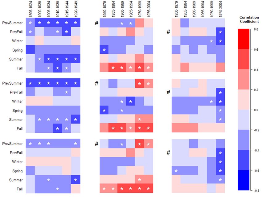
Forests 2019, 10, 1011                                                                               2 of 13

representing two distinct species [5,6]. At high elevation, two species co-occur, Pinus arizonica Engelm.
and the closely related P. ponderosa Lawson & Lawson var. brachyptera (Engelm.) Lemmon. The latter
species is also known as Taxon X, and the taxa are clearly distinguishable by needle traits with high
heritability [5–8]. P. ponderosa var. brachyptera exists in two forms, a nearly pure three-needle type
that survives at the highest altitudes on southern slopes (2300–3000 m), northern slopes, and cold air
drainages, and a mixed-needle type that is interspersed with the three-needle type at transition zones.
P. arizonica is a five-needle type found at lower elevations (below 2600 m). Thus, the five-needle pine
is more successful at warmer and drier, lower elevations, whereas the three-needle pine survives at
colder and wetter, higher elevations. On steep southern slopes the sharp transition of species occurs
over just c.130 m slope distance [6,9].
      We combined our dataset with Hal Fritts’ Mt. Bigelow chronologies [10–12], part of an
earlier meta-analysis which consisted of the three co-occurring taxa (three-needle, mixed-needle,
and five-needle types) sampled across a narrow climate gradient. We sampled the same population
c. 50 years later for a comparative analysis of similar aged cohorts, and also sampled the less dry
Mt. Lemmon location to determine the effect of site conditions on growth responses. Our goal
was to determine whether the climate–growth relationships have changed over the last century.
Shifting seasonality or relationships with limiting factors would have implications for reliably predicting
the vulnerability of tree species and needle types to climate change, conservation management,
and climate reconstruction.
      Previously, we reported on the two species of ponderosa pine displaying different growth
responses to moisture stress that varied based on the microsite environment [13]. P. arizonica’s growth
was reduced for longer periods by drought than P. ponderosa var. brachyptera, and the climatic response
was greater at the site with higher soil moisture content (Mt. Lemmon). Since the turn of the
twentieth century, average temperatures have been steadily increasing globally [14], and regionally
(Figure 1). Because rising temperatures, variable precipitation (Figure 1) and predicted shifts in the
monsoon season will influence weather patterns and drought in the Southwestern United States [15],
we hypothesized that the seasonality of limiting factors will change over time. The objective of the
study was to compare the correlations of ring widths with temperature and precipitation to assess
shifts in the seasonality of climate–growth responses.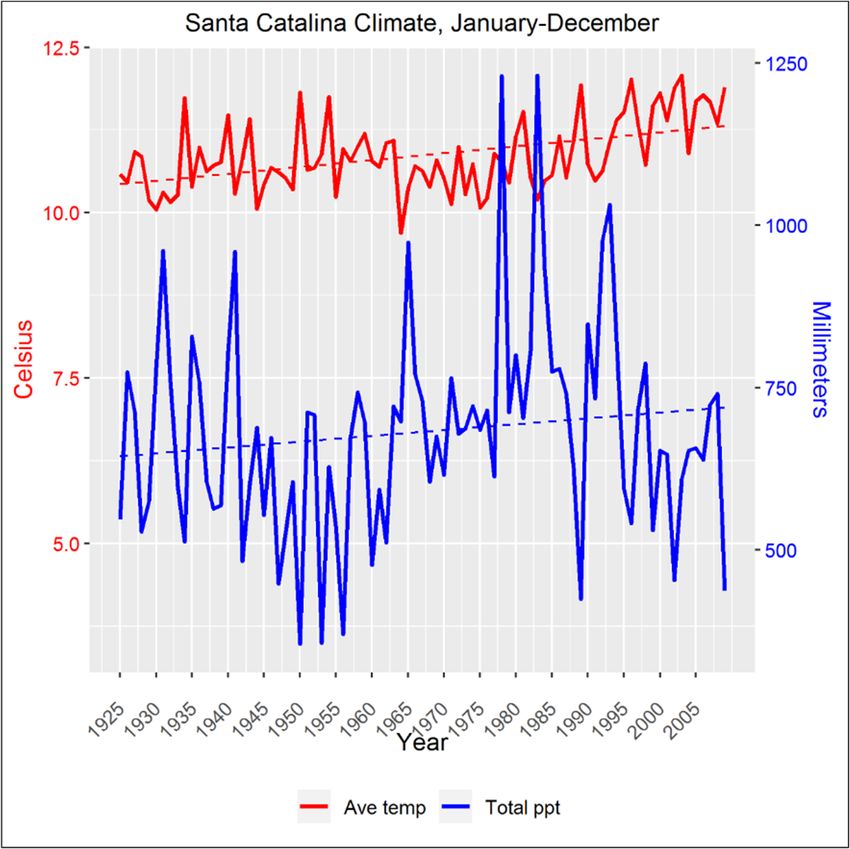
Forests 2019, 10, 1011 3 of 13
Forests 2019, 10, x FOR PEER REVIEW 3 of 13
Climate diagram
Figure 1. Climate diagram for
for the
the Santa
Santa Catalina
Catalina Mountains,
Mountains, for
for the
the 84-year
84-year reference
reference period spanning
1925–2009 for average annual temperature (Ave temp, ◦ C; red line) and total annual precipitation
temp,°C; total annual precipitation
(Total ◦ C over the course of the data set
(Totalppt,
ppt,mm;
mm;blue
blueline),
line),respectively.
respectively.The
TheAve
Avetemp
tempincreased
increasedbyby1.31.3 °C over the course of the data
(from ◦ C to 11.9 ◦ C). The dotted lines are the linear trend lines. Site-specific climatic data sets [Mt.
10.610.6
set (from °C to 11.9 °C). The dotted lines are the linear trend lines. Site-specific climatic data sets
Lemmon
[Mt. Lemmon(MTL), Mt. Bigelow
(MTL), (BIG)] (BIG)]
Mt. Bigelow [13,16] [13,16]
were validated with local
were validated climate
with localdata [13],data
climate and averaged
[13], and
to construct this diagram.
averaged to construct this diagram.
2. Materials and Methods
2. Materials and Methods
2.1. Study Area
2.1. Study Area
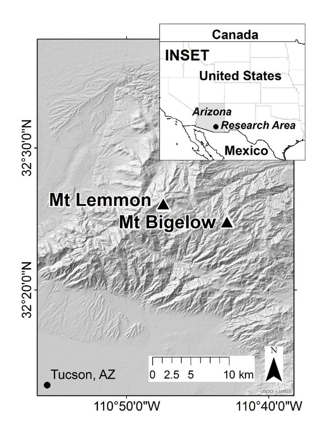
Tree-ring cores were sampled from two rugged southern slopes in the Santa Catalina Mountains
Tree-ring cores were sampled from two rugged southern slopes in the Santa Catalina Mountains
located 28 km northeast of Tucson, AZ, USA: Mt. Lemmon (MTL) and Mt. Bigelow (BIG; Figure 2).
located 28 km northeast of Tucson, AZ, USA: Mt. Lemmon (MTL) and Mt. Bigelow (BIG; Figure 2).
BIG (32.41, −110.71, 2534 m a.s.l.) is drier than MTL (32.43, −110.79, 2577 m a.s.l.), with average available
BIG (32.41, −110.71, 2534 m a.s.l.) is drier than MTL (32.43, −110.79, 2577 m a.s.l.), with average
water-holding capacities of 3.8% and 9.2%, respectively [13]. The climate of the desert southwest is
available water-holding capacities of 3.8% and 9.2%, respectively [13]. The climate of the desert
semiarid and warm with two rainy seasons, the summer monsoons (July through September) and
southwest is semiarid and warm with two rainy seasons, the summer monsoons (July through
winter cyclones (November through March) each delivering up to half of the annual precipitation to
September) and winter cyclones (November through March) each delivering up to half of the annual
the region [17]. P. arizonica, and P. ponderosa var. brachyptera (consisting of two-needle types described
precipitation to the region [17]. P. arizonica, and P. ponderosa var. brachyptera (consisting of two-needle
below) are dominant species in the mixed conifer forest. We selected archived samples from transition
types described below) are dominant species in the mixed conifer forest. We selected archived
zones where the three different needle types all grew together, which included the lower and upper
samples from transition zones where the three different needle types all grew together, which
moisture availability limits for P. ponderosa var. brachyptera and P. arizonica, respectively.
included the lower and upper moisture availability limits for P. ponderosa var. brachyptera and P.
arizonica, respectively.
Forests 2019, 10, x FOR PEER REVIEW 4 of 13
Forests 2019, 10, 1011 4 of 13
Figure 2. Locations of the two populations sampled for growth analysis: Mt. Lemmon (MTL) and
Figure
Mt. 2. Locations
Bigelow (BIG). of the two
Black populations
symbols sampled
locate study fornortheast
plots growth analysis: Mt. AZ
of Tucson, Lemmon
where(MTL) and Mt.
three-needle,
Bigelow (BIG). Black symbols locate study plots
mixed-needle, and five-needle pines are sympatric.northeast of Tucson, AZ where three-needle, mixed-
needle, and five-needle pines are sympatric.
2.2. Climate Data
2.2. Climate Data
The local meteorological stations provided only short but accurate climate records; thus, specific
The local meteorological
high-resolution gridded climatestations providedwere
(1 km) datasets onlydeveloped
short but accurate
using theclimate records;
ANUSPLIN thus, specific
package [16,18].
high-resolution
Climate gridded climate
dataset development and(1validation
km) datasets
werewere developed
described earlierusing
[13]. the ANUSPLIN
Climatic package
variables were
[16,18]. Climate
summarized dataset development
to monthly and validation
values of average were(TAVG),
temperature described earlierminimum
average [13]. Climatic variables
temperature
were summarized
(TMIN), to monthly
and total precipitation (PCP)values of they
because average temperature
were previously (TAVG),
found average drivers
to be significant minimum of
temperature
growth (TMIN),
responses [13]. and total precipitation (PCP) because they were previously found to be
significant drivers of growth responses [13].
2.3. Tree Growth Chronologies and Data Archives
2.3. Tree Growth Chronologies
We obtained tree-ring widthsand DataforArchives
P. arizonica [chronology (crn) 651000] and P. ponderosa var.
brachyptera
We obtained tree-ring widths for P. and
(three-needle type, crn 631000; mixed-needle
arizonica [chronology type, crn 651000]
(crn) 641000),and located at 2500 mvar.
P. ponderosa in
elevation
brachypteraon(three-needle
south-facing slopes, from
type, crn the Laboratory
631000; of Tree-Ring
and mixed-needle Research
type, (LTRR,
crn 641000), Tucson,
located AZ, USA;
at 2500 m in
Table S1; Figure S1). These early period (E) data (1881–1960) from BIG were acquired
elevation on south-facing slopes, from the Laboratory of Tree-Ring Research (LTRR, Tucson, AZ, as three composite
chronologies
USA; Table S1; thatFigure
had been S1). standardized with a (E)
These early period negative exponentialfrom
data (1881–1960) curveBIG
andwere
converted
acquiredto unit-less
as three
ring-width indices (RWI)that
composite chronologies [10–12] then standardized
had been trimmed to 1891–1949 for E analysis.
with a negative Archived
exponential curve andsamples were
converted
not available from MTL for an early period analysis.
to unit-less ring-width indices (RWI) [10–12] then trimmed to 1891–1949 for E analysis. Archived
In addition,
samples were notwe developed
available fromsixMTLnew forcomposite chronologies
an early period analysis. (three from BIG, three from MTL)
from Inraw ring widths archived with the International
addition, we developed six new composite chronologies (three Tree-Ring Data Bank
from BIG,(ITRDB;
three fromTable
MTL)S1,
Figures S2 and S3) [19]. The recent period (R; 1950–2007) raw chronologies
from raw ring widths archived with the International Tree-Ring Data Bank (ITRDB; Table S1, Figures did not overlap (in
time scale)
S2 and S3)with
[19].early
The period to simplify
recent period the response,
(R; 1950–2007) rawandchronologies
were de-trended using
did not a modified
overlap negative
(in time scale)
exponential curve to remove juvenile and geometric age trends, then
with early period to simplify the response, and were de-trended using a modified negative converted to standardized
ring-width
exponentialindices
curve using
to remove the ARSTAN program
juvenile and [20]. age
geometric The trends,
mean chronologies
then converted [computed by ARSTAN
to standardized ring-
(Tucson, AZ, USA)
width indices or acquired
using the ARSTAN from the LTRR] [20].
program were The
visualized
mean by using plotting
chronologies functionsbyinARSTAN
[computed the dplR
package
(Tucson,[21,22]
AZ, USA)for Ror [23].
acquired from the LTRR] were visualized by using plotting functions in the
dplR package [21,22] for R [23].Forests 2019, 10, 1011 5 of 13
The objective of this study was to compare the recent period tree-ring data with the analysis
conducted c. 50 years ago by Fritts [11,12], while using the same age of trees for the analysis.
Expressed Population Signal (EPS) measures the common variability of a composite chronology and for
early period was c. 0.89–0.96, indicating a strong common signal (see Appendix A for EPS thresholds).
The recent chronologies comprised of a minimum of six trees of each needle type (EPS 0.82–0.90) were
selected from the larger archived dataset [19]. Trees were characterized by average needle number
per fascicle (Table 1) reported for the selected individuals [13]. Trees that averaged >4.6 needles per
fascicle were designated P. arizonica [24], and P. ponderosa var. brachyptera contained two taxa identified
as a mixed-needle tree (3.2 ≤ mean ≤ 4.6 needles per fascicle), and a three-needle tree (Forests 2019, 10, 1011 6 of 13
temperature (TAVG) were divided into four seasons of three months each: winter (January-March),
spring (April-June), summer (July-September), and fall (October-December). The previous summer
and fall seasons were also considered, which increased the number of seasons analyzed to six.
Temporal instability of the moving correlation functions was tested with G-test to determine which time
series fluctuations were significantly different from those of a random time series [26]. The treeclim
results of the moving window analyses were plotted using functions in the ‘corrplot’ package [27]
for R.
3. Results
3.1. Seasonal Climate–Growth Relationships
Current spring PCP was the strongest predictor of tree growth for all needle types for BIG-R
(average r = 0.27 ± 0.04) and MTL-R (average r = 0.36 ± 0.04) after 1950. The strongest growth responses
were positive, producing significant correlations with spring PCP for all needle types at both sites for
the recent period (Table 2). In contrast, significant positive PCP-growth correlations were observed in
summer rather than spring for BIG-E for all needle-types (average r = 0.29 ± 0.03; Table 2). The response
function analysis (independent of period and location) indicated that 67% (4 out of 6) of mixed- and
five-needle type populations recorded a significant climate signal during winter prior to the growing
season (Table 2). For the two periods, significant positive PCP-growth correlations in winter were
observed only for BIG-E (average r = 0.24 ± 0.04) and at MTL-R (average r = 0.33 ± 0.03) and only for
mixed- and five-needle types. Winter precipitation was averaged between sites for two years with
contrasting moisture patterns. The winter of 1961 was one of the driest on record (137.2 mm), but the
following year (1962) was of normal moisture conditions (319.43mm). Considering mean ring-width
indices, growth for the five-needle type was 41% greater on average in 1962 than in 1961 (Table 3).
A smaller increase in growth occurred for the three-needle type (26%) and mixed-needle type (19%).
Table 2. Seasonal precipitation-growth relationships were determined by principal components
multiple regression for three taxa [three-needle (3N), mixed-needle (MN), five-needle (5N)] growing at
two transition zones [Mt. Bigelow (BIG), (Mt. Lemmon (MTL)] within the Santa Catalina Mountains.
Early Recent Recent
Taxa BIG (1891–1949) 2500 m BIG (1950–2007) 2534 m MTL (1950–2007) 2577 m
PrSum Win Spr Sum PrSum Win Spr Sum PrSum Win Spr Sum
3N - - - 0.32 - - 0.32 - - - 0.32 -
MN - 0.26 - 0.29 - - 0.26 - - 0.35 0.38 -
5N - 0.21 - 0.26 - - 0.24 - - 0.31 0.39 -
PrSum = previous summer (July–September); Win = winter (November–March); Spr = spring (April–June); Sum
= summer (July–September). The standard index composite chronologies analyzed were BIG-E for the early (E)
period of 1891–1949, and BIG-R and MTL-R for the recent (R) period of 1950–2007. Only significant correlations are
reported. All coefficients and confidence intervals are reported in Table S2.Forests 2019, 10, 1011 7 of 13
Table 3. Average (AVE) and standard deviation (SD) of mean ring-width indices and percent difference
(% DIFF) in growth between one dry winter (1961) and one normal winter (1962) for three-needle,
mixed-needle, and five-needle types at two transition zones [Mt. Bigelow (BIG), (Mt. Lemmon (MTL)]
within the Santa Catalina Mountains.
Three-Needle Type
Year BIG-R MTL-R AVE SD % DIFF
1961 731 769 750.0 026.9
1962 1000 886 943.0 080.6 26
Mixed-Needle Type
Year BIG-R MTL-R AVE SD % DIFF
1961 832 673 752.5 112.4
1962 967 828 897.5 098.3 19
Five-Needle Type
Year BIG-R MTL-R AVE SD % DIFF
1961 716 627 671.5 062.9
1962 966 898 932.0 048.1 41
Growth data for each needle type were obtained from standardized chronologies developed for recent (R) period
tree-ring correlation analyses.
3.2. Temporal Stability of Climate–Growth Relationships
The PCP–growth relationships were stable; the G-tests for PCP are non-significant (p > 0.05) for all
needle types analyzed across sites and periods (BIG-E; BIG-R; MTL-R; data not shown). Because these
correlation results supported the response function analysis reported above, we have only shown data
for the PCP response function analysis.
The TAVG–growth relationship was stable from 1895–1949 for BIG-E across needle types (i.e., G-test
p-values > 0.05; Figure 3A). The season with the largest number of individual significant negative
correlations (c. < −0.4; α = 0.05) was PrSum(April–June; i.e., summer of the previous year) with 4–6
correlations (out of 6), followed by Summer with 2–5 correlations (out of 6). In contrast, the relationship
between TAVG and growth became unstable during the recent period from 1960 to 2004 (p ≤ 0.05;
Figure 3B,C). This instability was indicated by significant G-tests (denoted by #), and changes in sign
for seasonal TAVG–growth correlations, from negative to positive for PrSum for BIG-R (Figure 3B)
and from positive to negative for PrevFall (July–September; i.e., fall of the previous year) at MTL-R
(Figure 3C) across all three needle types. For BIG-R, the fall season had the greatest frequency of
significant positive correlations (c. > 0.4; α = 0.05) with 5–6 correlations (out of 6). In comparison,
the growth of MTL-R trees experienced mostly negative correlations with TAVG. The season with the
largest number of significant negative correlations (c. < −0.4; α = 0.05) was winter with 1–2 correlations
(out of 6) for all needle types.Forests 2019, 10, 1011 8 of 13
Forests 2019, 10, x FOR PEER REVIEW 8 of 13
3-needle
mixed-needle
5-needle
(A)BIG-E (B) BIG-R (C) MTL-R
Figure 3. Moving
Figure window
3. Moving window correlation
correlationcoefficients for seasonal
coefficients for seasonalaverage
average temperature
temperature (TAVG)–growth
(TAVG)–growth
relationships for for
relationships three different
three differentneedle types,across
needle types, acrosstwo two
timetime periods
periods (Early(Early (E), (R))
(E), Recent Recent (R)) at
at two
two transition zoneswithin
transition zones withinthethe Santa
Santa Catalina
Catalina Mountains.
Mountains. From
From top top toare
to bottom bottom are correlations
correlations for three- for
needle, mixed-needle,
three-needle, mixed-needle, and
andfive-needle
five-needletypes, with
types, columns
with (A–C)
columns designating
(A–C) site and
designating sitetime period.
and time period.
Color scale = correlation coefficients; significant correlations (p < 0.05) are denoted by *. Intervals
Color scale = correlation coefficients; significant correlations (p < 0.05) are denoted by *. Intervals with
with low
low correlations
correlations(c.(c.
+0.2) are are
+0.2) shaded pale pale
shaded red orred
pale
orblue,
palewith
blue,the color
with theintensity increasingincreasing
color intensity with
correlation strength. Within time periods significant G-tests are denoted by #, which indicates
with correlation strength. Within time periods significant G-tests are denoted by #, which indicates
significant variability in the TAVG growth relationship over the time period (i.e., a sign of temporal
significant variability in the TAVG growth relationship over the time period (i.e., a sign of temporal
instability). Seasons fall along the y-axis, which are defined as PrSum = (April–June), PrevFall = (July–
instability). Seasons fall along the y-axis, which are defined as PrSum = (April–June), PrevFall =
September), Winter = (October–December), Spring = (January–March), Summer = (April–June), and
(July–September), Winter = (October–December), Spring = (January–March), Summer = (April–June),
Fall = (July–September). The standard index was used in the growth analyses. Confidence intervals
and Fall =
are reported in Table S3. The standard index was used in the growth analyses. Confidence intervals
(July–September).
are reported in Table S3.
4. Discussion
4.1. Seasonal Climate-Growth Relationships
Our chronology analysis highlighted a dramatic shift in annual growth in response to climatic
changes since the late 1950s [28]. Early period Mt. Bigelow ring widths correlated most strongly with
summer precipitation, indicating moisture conditions were sufficient for stomatal conductance and
annual growth to occur during the entire summer season [29], thus maximizing biomass production.
In comparison, recent climate–growth relationships were cool season correlations that occur when
trees restrict their wood production to early spring while conditions are favorable for growth at
dry sites [12,29] Thus, our recent season data indicated spring precipitation was the most important
variable for tree growth, which is also a crucial time for the formation of male and female reproductive
structures. These results support our hypothesis that the seasonality of climate variables important to
annual growth has shifted over time. We also found that winter precipitation was correlated with theForests 2019, 10, 1011 9 of 13
growth of mixed- and five-needle types, but not with growth of the three-needle type, suggesting the
three taxa have different ecological requirements for growth at their contact zone.
We report important fundamental differences within and between species in seasonal response to
climate, which suggest that adaptation of tree species to length of growing season may have occurred.
These results support the influence of historical precipitation patterns and climate restrictions for
different taxa [30,31]. The length of growing season of P. ponderosa in Nevada was controlled entirely
by moisture conditions and not temperature by monitoring the cambial activity for two consecutive
years with contrasting moisture, one wet winter and one dry spring [32]. Summer precipitation was
not used by the trees unless the start of the growing season was delayed by dry winter and/or spring
conditions. Because moisture availability determines the length of growing season for all needle types
of ponderosa pine studied in the Santa Catalina Mountains [13], we hypothesize that one taxon may
optimize growth over a shorter or longer growing season (five-needle, three-needle, respectively) [10],
and a third taxon may grow best under a variable growing season (mixed-needle), which we call the
dry cool-season hypothesis.
In support of this dry cool-season hypothesis, cambial activity was measured during the dry 1961
growing season [10]; the average Palmer Drought Severity Index (PDSI), a measure of soil moisture
availability [33], was c. −3.0 [13]. [More negative values of PDSI indicate drought stress and range from
-4 to +4]. The cambial expansion of P. ponderosa var. brachyptera (the three- and mixed-needle types)
initiated under dry winter conditions in February, followed by the five-needle type (P. arizonica) six
weeks later in April. Cambial growth occurred for all needle types during the summer, and cessation
of growth coincided in September. All needle types co-existed at the Mt. Bigelow transition zone
(2500 m a.s.l.) including trees that were analyzed for climatic response in this study and the prior
study [11]. Although the initiation of radial growth for the following normal moisture year (average
PDSI c. −0.5) [13] was not determined, we can predict the growth response of the five-needle type
to wet winter conditions from the recent literature on moisture driven cambial activity described
above [32]. Because the five-needle type responds positively to winter precipitation, the taxon should
initiate growth earlier. Further support was provided by our chronology data, which showed that
growth for the five-needle type is robust when winter moisture conditions are normal (compared to
dry winter). Also, a 15–22% increase in growth for the five-needle type was observed above that for
the three- and mixed-needle types, respectively, for normal moisture winter. This increase in growth
is suggestive that five-needle type starts cambial expansion earlier in wet springs than dry springs
and supports our earlier study [13] that found the five-needle pine responded positively to PDSI for
longer periods of time. Long correlation with PDSI suggests a possible adaptation to drought under a
mechanism that 5-needle trees grow only when there is a reliable water source. Therefore, our study
results reinforce that moisture availability determines the length of growing season of ponderosa pine,
and that some needle types may display variability in the timing of xylogenesis [32].
4.2. Temporal Stability of Climate–Growth Relationships
We found opposing growth trends in response to temperature after 1950 between the two sites,
which indicates that combining tree-ring data from multiple sites into a single chronology can dilute
the individual climate signals. Opposing temperature–growth trends were first reported in white
spruce stands occurring at the tree-line in two mountain ranges sampled across Alaska, and that
temperature explained more variability in annual tree growth post-1950 [34]. These regional Alaskan
forests are composed of individual trees growing in heterogeneous environments where temperature
thresholds operate, influencing tree biology and the response to limiting factors that appears in the
final chronology. Our report extends these tree-line studies to semiarid regions where precipitation
rather than temperature is the factor most limiting to tree annual growth. Nonetheless, we also
observed a significant shift from positive to negative growth correlations with temperature under less
dry conditions for five-needle and mixed-needle types during cool seasons, which is indicative of
temperature-induced drought stress [34], or growing season respiration [13] limiting the ponderosaForests 2019, 10, 1011 10 of 13
pine annual growth. In comparison, at the drier site we observed a shift from negative to positive
temperature correlations during PrSum season post-1950, indicating reduced water stress. Furthermore,
if unaccounted for, these opposing trends to temperature are weakening the warming climate signal
(post-1950) by combining positive and negative growth responses that adversely affect growth response
analyses and by extension climate reconstructions based on ring-width data, even in dry environments
where precipitation is growth limiting.
Also, by extending our analysis to include the fall season, we observed that growth in individual
trees is positively and significantly correlated to temperature. These results suggest that all needle types
may respond positively to a range of temperature increases late in the season at the contact zone of dry
habitats. However, an extended growing season most likely will be determined by moisture availability
and not rising temperatures, as recently described for P. ponderosa, a closely related species [32].
5. Conclusions
A temporal shift in limiting factor indicated spring is the most important growing season for
recent period; thus, the three taxa that responded to summer precipitation pre-1950 are now responding
to spring precipitation post-1950. This shift in limiting factor represents a shift in allocation of
tree resources from maximizing biomass (summer) to reproduction (spring), a critical time for tree
phenology and the formation of male and female reproductive structures. Five- and mixed-needle
types correlated positively to winter precipitation, suggesting soil moisture was controlling the length
of growing season. Also, we found significant fluctuations in temperature–growth correlations during
recent period for all needle types. Thus, a shift in limiting factor that impacts the growth sensitivity
of trees, such as warming trends that increase local moisture stress, may also impact the stability
of climate–growth relationships, and if unaccounted for, obscures the use of tree-rings to analyze
temperature–growth responses and reconstruct climate on moisture-limited sites.
Supplementary Materials: The following are available online at http://www.mdpi.com/1999-4907/10/11/1011/s1,
Table S1: Ponderosa pine tree-ring data archives, Table S2: Coefficients and confidence intervals for Table 2’s
response function seasonal precipitation–growth analysis, Table S3: Coefficients and confidence intervals for
Figure 3’s moving window seasonal TAVG growth analysis, Figure S1: Average yearly standard chronology for
three-needle, mixed-needle, and five-needle types in the early BIG tree-ring study [10,11], Figure S2: Average
yearly standard chronologies for three-needle, mixed-needle, and five-needle types in the recent BIG tree-ring
study, Figure S3: Average yearly standard chronologies for three-needle, mixed-needle, and five-needle types in
the recent MTL tree-ring study.
Author Contributions: P.E.M. conceived the study, designed the experiments, and analyzed data; B.R.M. assisted
with data analysis; F.W.T. contacted the LTRR to obtain historical tree-ring data files; P.E.M. wrote the paper; F.W.T.
and B.R.M. edited the paper.
Funding: The USDA Forest Service, Northern Research Station, and the Department of Plant Biology, Michigan
State University provided financial support for this research project.
Acknowledgments: This paper is part of a dissertation submitted to Michigan State University in partial
fulfillment of requirements for a Doctor of Philosophy degree. We thank the following people for help on the
project: M. Munro and C. Baisan supplied H. Fritts’ chronology samples. J. Stanovick provided statistical support.
H. Jenson provided GIS support. D. Donner reviewed the paper.
Conflicts of Interest: The authors declare no conflict of interest.
Appendix A
Defining Chronology Confidence and EPS Thresholds
Analysis of variance (ANOVA) and correlation-derived estimates of population parameters require
a minimum of five single-core series and 30-annual rings to provide accurate values for tree-ring
statistical analysis [35]. Therefore, we selected 6–7 trees (two or more cores per tree), setting a minimum
length limit of a 47-year common interval to construct composite chronologies for each group of trees
(Table S1; Figures S2 and S3). The percent variance component for the group chronology VC(Y) as
determined by analysis of variance is equivalent to the between tree correlation rbt of correlationForests 2019, 10, 1011 11 of 13
tree-ring analysis [35,36]. Rbt measures the common signal strength and is dependent on sample
depth [37]. Expressed Population Signal (EPS) is a measure of statistical quality to help produce a
reliable population level estimate of the climate signal, and is dependent on rbt [35]
t rbt
EPS =
t x rbt + (1 − rbt )
Although the minimum EPS value of 0.85 is recommended by Wigley et al. [36] to be routinely
applied in dendrochronological analyses, we considered EPS values ranging from 0.82 to 0.90 for
each group of trees that included growth data from 1950 to 2007, which is a good reflection of overall
chronology confidence. Given that our study design includes a variable core depth, this method
of estimating the common chronology signal with a range of EPS values was simpler to apply.
The chronology signal describes the variance in common to all tree-ring series sampled and analyzed
at a specific site. This approach of using a range of EPS values was supported by Briffa and Jones’ [34]
suggestion that a minimum value may not represent the most appropriate estimate of chronology
confidence for all situations. For example, a 3% reduction in EPS from 0.85 to 0.82 would signify a
reduction of 2% in explained climate variance. Thus, for climate–growth relationships with 64–65%
of variance attributed to climate, as reported by Fritts [11] for the mixed- and three-needle types of
Ponderosae on Mt. Bigelow, an EPS threshold of 0.85 would have reduced the explained climate variance
to 55% (64.5% × 0.85). In comparison, an EPS threshold of 0.82 would have reduced the explained
variance to 53%. Therefore, the additional chronology error would have restricted the explained climate
variance by just 2%. Thus, it seems unlikely that an additional 3% reduction in chronology confidence
(from 0.85 to 0.82) would affect the estimation of the climate signal within needle types of standardized
chronologies, when sensitivities to climate are expected to be high, as in this study [10,11,13,36].
The EPS thresholds for Fritts’ [11] study can be estimated from formulas described by
Wigley et al. [37] as:
[N (%Y)]
SNR =
100 − %Y
SNR
EPS =
1 + SNR
where SNR is the signal to noise ratio, N is the number of series, and %Y is the percent common
variance [35]. As an example, when substituting 12 for N and 41 for %Y [11] (%EMS, from Table 1),
we derived SNR = 8.4 and EPS = 0.89 for the five-needle type of the prior Mt. Bigelow study. Similarly,
for the three-needle type, by substituting 65 for %Y [11] we derive an EPS value of 0.96. These values
approximate EPS of the current study, as 11 years of data were removed (1950 to 1960) from the
chronologies used for the early period analysis (BIG-E).
References
1. Warshall, P. The Madrean sky island archipelago: A planetary overview. In Biodiversity and Management of the
Madrean Archipelago: The Sky Islands of Southwestern United States and Northwestern Mexico; DeBano, L.F.,
Ffolliott, P.F., Ortega-Rubio, A., Gottfried, G.J., Hamre, R.H., Edminster, C.B., Eds.; US Department of
Agriculture: Fort Collins, CO, USA, 1995; pp. 6–18. [CrossRef]
2. Jump, A.S.; Hunt, J.M.; Penuelas, J. Rapid climate change-related growth decline at the southern range edge
of Fagus sylvatica. Glob. Chang. Biol. 2006, 12, 2163–2174. [CrossRef]
3. Tegel, W.; Seim, A.; Hakelberg, D.; Hoffmann, S.; Panev, M.; Westphal, T.; Büntgen, U. A recent growth
increase of European beech (Fagus sylvatica L.) at its Mediterranean distribution limit contradicts drought
stress. Eur. J. Forest Res. 2014, 133, 61–71. [CrossRef]
4. USGCRP. Climate Science Special Report: Fourth National Climate Assessment; Wuebbles, D.J., Fahey, D.W.,
Hibbard, K.A., Dokken, D.J., Stewart, B.C., Maycock, T.K., Eds.; U.S. Global Change Research Program:
Washington, DC, USA, 2017; Volume 1, p. 470. [CrossRef]Forests 2019, 10, 1011 12 of 13
5. Rehfeldt, G.E. Systematics and genetic structure of Ponderosae taxa (Pinaceae) inhabiting the Mountain
Islands of the Southwest. Am. J. Bot. 1999, 86, 741–752. [CrossRef] [PubMed]
6. Epperson, B.K.; Telewski, F.W.; Willyard, A. Chloroplast diversity in a putative hybrid swarm of Ponderosae
(Pinaceae). Am. J. Bot. 2009, 96, 707–712. [CrossRef] [PubMed]
7. Willyard, A.; Gernandt, D.S.; Potter, K.; Hipkins, V.; Marquardt, P.; Mahalovich, M.F.; Langer, S.K.;
Telewski, F.W.; Cooper, B.; Douglas, C.; et al. Pinus ponderosa: A checkered past obscured four species.
Am. J. Bot. 2017, 104, 161–181. [CrossRef] [PubMed]
8. Rehfeldt, G.E. Early selection in Pinus ponderosa: Compromises between growth potential and growth rhythm
in developing breeding strategies. Forest Sci. 1992, 38, 661–677. [CrossRef]
9. Epperson, B.K.; Telewski, F.W.; Plovanich-Jones, A.E.; Grimes, J.E. Clinal differentiation and putative
hybridization in a contact zone of Pinus ponderosa and P. arizonica (Pinaceae). Am. J. Bot. 2001, 88, 1052–1057.
[CrossRef] [PubMed]
10. Dodge, R.A. Investigations into the Ecological Relationships of Ponderosa Pine in Southeast Arizona.
Ph.D. Thesis, University of Arizona, Tucson, AZ, USA, 1963.
11. Fritts, H.C. Computer programs for tree-ring research. Tree-Ring Bull. 1963, 25, 2–7.
12. Fritts, H.C. Relationships of ring widths in arid-site conifers to variations in monthly temperature and
precipitation. Ecol. Monogr. 1974, 44, 411–440. [CrossRef]
13. Marquardt, P.E.; Miranda, B.R.; Jennings, S.; Thurston, G.; Telewski, F.W. Variable climate response
differentiates growth of the Sky Island ponderosa pines. Trees 2019, 3, 317–332. [CrossRef]
14. IPCC. 2007: Climate Change. The physical science basis. In Contribution of Working Group I to the Fourth
Assessment Report of the Intergovernmental Panel on Climate Change; Solomon, S., Qin, D., Manning, M., Chen, Z.,
Marquis, M., Averyt, K.B., Tignor, M., Miller, H.L., Eds.; Cambridge University Press: Cambridge, UK;
New York, NY, USA, 2007.
15. Pascale, S.; Boos, W.R.; Bordoni, S.; Delworth, T.L.; Kapnick, S.B.; Murakami, H.; Vecchi, G.A.; Zhang, W.
Weakening of the North American monsoon with global warming. Nat. Clim. Chang. 2017, 7, 806–812.
[CrossRef]
16. McKenney, D.W.; Hutchinson, M.F.; Papadopol, P.; Lawrence, K.; Pedlar, J.; Campbell, K.; Milewska, E.;
Hopkinson, R.F.; Price, D.; Owen, T. Customized spatial climate models for North America. Bull. Am.
Meteorol. Soc. 2011, 92, 1611–1622. [CrossRef]
17. Sheppard, P.R.; Comrie, A.C.; Packin, G.D.; Angersbach, K.; Hughes, M.K. The climate of the US Southwest.
Clim. Res. 2002, 21, 219–238. [CrossRef]
18. Hutchinson, M.; Xu, T. Anusplin Version 4.4 User Guide; Australia National University: Canberra, Australia, 2013.
19. Marquardt, P.E.; Miranda, B.R.; Telewski, F.W. (2018-01-18): NOAA/WDS Paleoclimatology - Mt. Bigelow
– PIAZ, PIPO – ITRDB AZ595-596 [Study 23650-23651]; Mt. Lemmon – PIAZ, PIPO – ITRDB AZ597-598
[Study 23652-23653]. NOAA National Centers for Environmental Information. Available online: https:
//www.ncdc.noaa.gov/paleo/study/xxxxx (accessed on 1 October 2018).
20. Cook, E.R. ATime Series Analysis Approach to Tree Ring Standardization. Ph.D. Thesis, University of
Arizona, Tucson, AZ, USA, 1985.
21. Bunn, A.G. A dendrochronology program library in R (dplR). Dendrochronologia 2008, 26, 115–124. [CrossRef]
22. Bunn, A.G. Statistical and visual crossdating in R using the dplR library. Dendrochronologia 2010, 28, 251–258.
[CrossRef]
23. R Core Team. R: A Language and Environment for Statistical Computing; R Foundation for Statistical Computing:
Vienna, Austria, 2016; Available online: https://www.R-project.org/ (accessed on 1 October 2018).
24. Peloquin, R.L. The identification of three-species hybrids in the ponderosa pine complex. Southwest. Nat.
1984, 29, 115–122. [CrossRef]
25. Rehfeldt, G.E. Genetic variation in the Ponderosae of the southwest. Am. J. Bot. 1993, 80, 330–343. [CrossRef]
26. Zang, C.; Biondi, F. Treeclim: An R package for the numerical calibration of proxy-climate relationships.
Ecography 2015, 38, 431–436. [CrossRef]
27. Wei, T.; Simko, V. R Package “Corrplot”: Visualization of a Correlation Matrix (Version 0.84). 2017.
Available online: https://github.com/taiyun/corrplot (accessed on 1 October 2018).
28. Kienast, F.; Luxmoore, R.J. Tree-ring analysis and conifer growth responses to increased atmospheric CO 2
levels. Oecologia 1988, 76, 487–495. [CrossRef] [PubMed]Forests 2019, 10, 1011 13 of 13
29. Lévesque, M.; Rigling, A.; Bugmann, H.; Weber, P.; Brang, P. Growth response of five co-occurring conifers to
drought across a wide climatic gradient in Central Europe. Agri. Forest Meteorol. 2014, 197, 1–12. [CrossRef]
30. Kilgore, J. Distribution and Ecophysiology of the Ponderosae in the Santa Catalina Mountains of Southern
Arizona. Ph.D. Thesis, Michigan State University, East Lansing, MI, USA, 2007.
31. Norris, J.R.; Jackson, S.T.; Betancourt, J.L. Classification tree and minimum-volume ellipsoid analyses of the
distribution of ponderosa pine in the western USA. J. Biogeogr. 2006, 33, 342–360. [CrossRef]
32. Ziaco, E.; Truettner, C.; Biondi, F.; Bullock, S. Moisture-driven xylogenesis in Pinus ponderosa from a Mojave
Desert mountain reveals high phenological plasticity. Plant Cell Environ. 2018, 41, 823–836. [CrossRef]
[PubMed]
33. Palmer, W.C. Meteorological Drought; U.S. Weather Bureau Research Paper No. 45; US Department of
Commerce: Washington, DC, USA, 1965; Volume 30, pp. 1–58.
34. Wilmking, M.; Juday, G.P.; Barber, V.A.; Zald, H.S. Recent climate warming forces contrasting growth
responses of white spruce at treeline in Alaska through temperature thresholds. Glob. Chang. Biol. 2004, 10,
1724–1736. [CrossRef]
35. Briffa, K.; Jones, P. Basic Chronology statistics and assessment. In Methods of Dendrochronology; Cook, E.R.,
Kairiukstis, L.A., Eds.; Springer Science Business Media B.V: Dordrecht, The Netherlands, 1990; pp. 137–152.
ISBN 978-90-481-4060-2.
36. Fritts, H.C. Tree Rings and Climate; Academic Press Inc.: London, UK, 1976; ISBN 0 12 268450-8.
37. Wigley, T.M.L.; Briffa, K.R.; Jones, P.D. On the average value of correlated time series, with applications in
dendroclimatology and hydrometeorology. J. Clim. Appl. Meteorol. 1984, 23, 201–213. [CrossRef]
© 2019 by the authors. Licensee MDPI, Basel, Switzerland. This article is an open access
article distributed under the terms and conditions of the Creative Commons Attribution
(CC BY) license (http://creativecommons.org/licenses/by/4.0/).You can also read