Phase Planning for Open Pit Coal Mines through Nested Pit Generation and Dynamic Programming

Hindawi
Mathematical Problems in Engineering
Volume 2021, Article ID 8219431, 8 pages
https://doi.org/10.1155/2021/8219431

Research Article
Phase Planning for Open Pit Coal Mines through Nested Pit
Generation and Dynamic Programming

 Xiaowei Gu, Qing Wang , Xiaochuan Xu, and Xiaoqian Ma
 College of Resources and Civil Engineering, Northeastern University, 110819 Shenyang, China

 Correspondence should be addressed to Qing Wang; qingwangedu@163.com

 Received 28 July 2020; Revised 26 January 2021; Accepted 28 January 2021; Published 11 February 2021

 Academic Editor: Zhengbiao Peng

 Copyright © 2021 Xiaowei Gu et al. This is an open access article distributed under the Creative Commons Attribution License,
 which permits unrestricted use, distribution, and reproduction in any medium, provided the original work is properly cited.

 This paper presents a phase planning method specially designed for coal deposits with nearly horizontal, bedded coal seams. The
 geology of this type of deposit is modeled into a column model, instead of a block model, to avoid coal-rock mixing in blocks. A
 nested pit generation algorithm is developed for producing a series of nested, least-strip ratio pits with a column model as its input.
 The algorithm completely overcomes the troublesome gap problem. Taking the least-strip ratio pits as possible phase states, a
 dynamic programming formulation is proposed to simultaneously optimize the number of phases, the phase-pits, and the
 ultimate pit, with an objective of maximizing the net present value. The merits and capability of the proposed method are
 demonstrated through a case study on a large coal deposit.

1. Introduction of “technically optimal pits.” A technically optimal pit for a
 total volume, V, and ore quantity, Q, is the pit that has the
Large open pit mines are often mined in a number of phases, highest quantity of mineral of interest among all pits of the
with intermediate pits for the phases referred to as phase-pits same V and Q. A number of authors have elaborated on the
or pushbacks. The phases must be carefully planned since mathematical formulations and solution algorithms for
they provide a long-term strategic guide for the sequential technical parameterization of reserves [2–7]. Dagdelen and
development of a mine and for detailed production Johnson formulated the pushback optimization problem
scheduling. In designing the phases, three elements must be into an integer programming (IP) model and used La-
determined: the number of phases, the phase-pits, and the grangian relaxation for solution [8]. All these methods have
ultimate pit. These elements are interrelated and should be an inherent gap problem; that is, the size increment between
simultaneously optimized to maximize the net present value two consecutive pits can be very large. Big gaps can inflict
(NPV) of an open pit project. serious difficulties when the pits are used for phase planning
 Phase optimization, unlike production scheduling, has or production scheduling, with the resulting solution far
not been an extensively studied topic in open pit planning in from the optimal or with no feasible solution at all. To
recent years, and most of the research work had been done overcome the gap problem, Wang and Sevim proposed a
before the turn of the century. Lerchs and Grossmann first heuristic algorithm using a cone eliminating process [9]. The
introduced the parametric analysis approach, where the algorithm is capable of finding a series of nested, maximum-
block values of the block model are systematically changed metal pits with a pit increment almost the same as the user
and a pit optimization algorithm is executed repeatedly to specified value and, thus, completely eliminates the gap
obtain an optimal pit each time after the block values are problem. Meagher et al. formulated the pushback optimi-
changed, producing a series of nested pits [1]. These pits can zation problem as an IP model [10]. To facilitate the solution
then be evaluated to choose the appropriate phase-pits. process and to overcome the gap problem, they solved the
Technical parameterization of reserves is another method for linear programming relaxation version of the IP model first
nested pit generation, with an objective of finding the family and, then, applied a method known as “pipage rounding” to

2 Mathematical Problems in Engineering

convert a fractional solution into an integral solution. The Based on the basic framework from a previous research
authors claimed that their approach completely overcomes for metal mines [19], we have developed a phase planning
the gap problem. method particularly for open pit coal mines with nearly
 One of the most significant developments in the related horizontal and bedded coal seams, with the objective of
and wider area of open pit planning, over the last two simultaneously optimizing the number of phases, the phase-
decades, is probably the incorporation of geological un- pits, and the ultimate pit.
certainty in planning schemes. Conditional geostatistical
simulation techniques have been developed that are ca- 2. Coal Deposit Modeling: the Column Model
pable of generating multiple, equally probable, realizations
of an orebody [11–14]. These realizations show the possible Almost all open pit optimization formulations and solution
variations of the mineral content and corresponding algorithms take 3D block models of deposits as their geo-
tonnages of a deposit and provide the basis for quantifying logical inputs. However, most coal deposits consist of nearly
geological uncertainty. Based on simulated orebody real- horizontal (inclination angle smaller than 15° or so), bedded
izations, stochastic open pit planning techniques can be coal seams. As depicted in Figure 1, blocks at the coal-rock
used to integrate geological uncertainty into planning interfaces contain a mixture of coal and rock (e.g., the blocks
processes, so as to allow some sort of geological risk outlined by the dotted lines), and such blocks constitute a
management while maximizing the expected NPV. Several significant portion of all the blocks containing coal. This will
authors have incorporated geological uncertainty in their cause large errors in coal quantity calculation and subse-
pushback/phase-pit optimizing approaches. Goodfellow quent economic evaluation, since whole blocks are classified
and Dimitrakopoulos applied the simulated annealing al- as coal or waste. The problem is more pronounced in cases of
gorithm to pushback design based on simulated orebody multiple coal seams and/or the coal seams are thin.
realizations [15]. Their goal was to modify an existing In this study, we model this type of coal deposit into a
 “
pushback design to better account for the joint local un- column model,” where the whole deposit is divided into
certainty in metal grades and material types, while vertical columns instead of blocks, with all columns having a
remaining similar to the original design in terms of square horizontal cross section of the same size. Figure 1
pushback tonnages and the tonnages sent to various des- illustrates a vertical cross section of a column model with the
tinations. Their case study on a copper mine showed that columns numbered from 1 to 23. Each column in such a
the approach achieved a 35–61% reduction in variability in model is assigned a group of attributes defining the physical
terms of material quantities sent to the processes, leading to and chemical properties of all the coal seams along the
a reduced level of risk in the economic value of the design. column. The attributes generally include floor elevation and
Asad and Dimitrakopoulos presented a stochastic para- thickness of each coal seam and the unconsolidated layer at
metric maximum flow algorithm for pushback design the central line of the column, and heat value, ash content,
under uncertainties in both metal content and commodity and sulfur content of each coal seam along the column.
price [16]. They used Lagrangian relaxation together with These attributes may be estimated based on drill hole data
subgradient method to accommodate knapsack constraints using a method such as Kriging or inverse distance inter-
for ore quantities in the pushbacks and addressed the gap polation. With a column model, the coal quantity in any
problem by introducing a modification in the subgradient given volume (e.g., a pit or a cone) is calculated based on the
method to minimize the size difference between consec- thickness of each seam falling inside the volume on each
utive pushbacks. The authors applied the algorithm to a column. The resulting coal quantity is much more accurate
gold mine and compared the outcome with that from the than that based on whole blocks with a block model. The
conventional (deterministic) nested pit approach [17]. The reduction in coal-rock mixing with a column model, as
case study demonstrated that the stochastic approach gave compared with a block model, depends on the geometries of
30% more discounted cash flow, a 21% larger ultimate pit, the coal seams (especially, their thicknesses) and the block
and about 7% more metal than the conventional approach. and column sizes. For the coal deposit model used in the case
Asad et al. later expanded the formulation to include study, we estimated that the reduction is at least 50% in
multiple ore processing streams [18]. terms of the total amount of rock mixed in coal and coal
 As mentioned above, the number of phases, the phase- classified as waste.
pits, and the ultimate pit should be optimized simulta-
neously. However, few approaches are capable of providing 3. Generation of Least-Strip Ratio Pits
simultaneous solutions to the three elements, especially, for
coal mines. Asad and Dimitrakopoulos’ algorithm solves the The basic idea of phase optimization is first generating a
phase-pits and ultimate pit simultaneously, but the gap candidate series of nested pits with a specified size increment
problem is not completely overcome and the algorithm is for and, then, selecting the best phase-pits (including the ulti-
metal mines [16]. Gu et al. proposed a method capable of mate pit) from the series that maximize the NPV. The best
providing simultaneous solutions to the three elements [19]. candidate pits are the least-strip ratio pits, referred to as
 “
It consists of a heuristic algorithm for generating a series of least-SR pits” hereafter. A least-SR pit for a given coal
geologically optimal pits and a dynamic programming (DP) quantity, Q, is defined as the pit that has the lowest strip ratio
formulation for sequencing the pits, but the method is also of all pits having the same Q. To overcome the gap problem,
for metal mines. a cone eliminating algorithm is applied on a column model

Mathematical Problems in Engineering 3

 Ground surface Unconsolidated layer quantities of coal, rock, and unconsolidated material in the
 cone inside pit Pi. The cone’s coal quantity is denoted as qc. If
 qc is not greater than the coal quantity increment, ΔQ,
 specified for the pit series, compute the cone’s strip ratio and
 put the cone in an array. Then, move the cone apex upwards
 Seam 1 along the central line of the same column by a distance of Δz,
 and do the same as for the previous cone. Continue the
 Seam 2
 process of moving the cone upwards along the same column,
 1 3 5 7 9 11 13 15 17 19 21 23 until the cone’s coal quantity, qc, is greater than ΔQ, or the
 cone’s apex is above the ground surface, as depicted by the
 Blocks containing a mixture of coal and rock if a block upward arrow and the dot lined cones in Figure 2. Then, the
 model were to be used
 cone is moved horizontally to another column inside pit Pi,
Figure 1: Illustration of a vertical cross section of a column model. as shown by the horizontal arrow in Figure 2, and the entire
 process for the previous column is repeated. The above
to generate a series of nested, least-SR pits. The basic logic of process continues until all the columns inside pit Pi are
the algorithm is briefly described as follows. traversed.
 Suppose that a series of n nested, least-SR pits, denoted At the end of the above cone moving process, an array
as {P}n P1 , P2 , . . . , Pn , is to be generated with a specified of J cones, each having a coal quantity qc ≤ΔQ, is obtained.
coal quantity increment of ΔQ, where P1 is the smallest pit Sort the cone array in order of descending strip ratio. A
and Pn the largest. Let Qi denote the coal quantity in Pi. The union of the first K cones in the sorted cone array is
algorithm starts with the largest pit, Pn, which is created by sought, such that the total coal quantity of the union is
projecting the pit walls from a closed surface boundary closest to ΔQ and not greater than 1.1ΔQ. In a cone union,
outline down to the lowest floor elevation of the lowest coal the overlapping part between two or more cones is
seam, according to the pre-determined slope angles in accounted only once. Such a union is obtained by se-
different directions or in different zones. The pit slope angles quentially combining the cones in the sorted array one at a
are determined beforehand through rock stability studies time, starting with the first cone. The cones in the union
and are inputs to the algorithm. The surface boundary could are eliminated from pit Pi and the remaining part is pit
be the boundary that encloses all exploration drill holes, or Pi−1, whose coal quantity is about ΔQ smaller than Pi.
the property boundary for which the mining company has Eliminating a cone from a pit is simply done by raising the
acquired the right of mining, or any boundary that is large bottom elevation of each column traversed by the cone up
enough to enclose the optimal ultimate pit within the ac- to the cone shell elevation at the column center.
quired property. Within Pn, the algorithm searches for a The algorithm outlined above is a heuristic one and does
portion that contains a coal quantity of ΔQ and has the not guarantee that the resulting pit is the true least-SR pit.
highest strip ratio, and then eliminates this portion from Pn. However, since the eliminated cones are the ones having the
The remaining part of Pn after eliminating such a portion highest strip ratios, their union constitutes a volume whose
constitutes the next smaller pit, Pn−1, in the series, which has strip ratio should be very close to the highest strip ratio of all
a coal quantity of Qn − ΔQ. To make Pn−1 feasible with re- volumes with the same coal quantity. Thus the remaining
spect to pit slope constraints, the eliminated portion is part should be very close to the true least-SR pit for its coal
constructed by combining upward cones (whose apexes quantity.
point upwards) with shell inclination angles equal to the pit In the above algorithm, each and every cone kept in the
slope angles. From Pn−1, the same cone eliminating process array has a coal quantity not greater than the specified
is repeated to generate the nest smaller pit, Pn−2. The process increment, ΔQ, and the coal quantity of the eliminated cone
continues until the coal quantity in the remaining part is union is controlled by an upper limit of 1.1ΔQ. Thus, the coal
equal to or below the coal quantity, Q1, specified for the quantity increment between any consecutive pits in the
smallest pit in the series, thus, resulting all the pits in the generated pit series may be smaller than ΔQ, but cannot
series. exceed 1.1ΔQ. The gap problem is, therefore, completely
 With a column model, a pit is outlined by the bottoms overcome.
and the tops of all the columns inside the pit, as depicted in The up-moving step size, Δz, can affect the quality of the
Figure 2 for pit Pi, where the bottom elevation of each resulting pits: a smaller Δz generally gives better result (i.e.,
column is equal to the elevation of the pit wall or pit bottom the resulting pits are closer to the true least-SR pits), but
at the column center, and the top elevation of each column is consumes more time and memory. Δz is an input parameter
equal to the elevation of ground surface at the column to the developed software and different values can be tried if
center. Without losing generality, suppose we have come to necessary. From our experiments on different coal deposits
the point of generating Pi−1 from pit Pi. The cone eliminating using different Δz values, bench height, h (usually
process is outlined as follows. 10 m−15 m), is a good choice for Δz, and smaller values (e.g.,
 Place the cone apex on the central line of a column at an h/2, h/4) make insignificant improvement on the resulting
elevation that is Δz higher than the bottom elevation of the pits, but substantially increase the computing time. The
column, as shown by Cone 1 in Figure 2. Calculate the column size has a similar effect.

4 Mathematical Problems in Engineering

 1 2 3 4 5 6 7 8 9 10 11 12 13 14 15 16 17 18 19 20 21 22

 Unconsolidated layer

 Cone Seam 1
 moving Δz
 Seam 2
 upwards
 Pi
 along a
 Seam 3
 column
 Cone 1
 Cone j
 Cone moving horizontally
 between columns

 Cone array in order of Cone J
 Cone 1 Cone 2 Cone j
 descending strip ratio
 Figure 2: Illustration of the cone eliminating process for generating nested, least-SR pits.

4. Dynamic Programming Formulation for P p6 p6 p6 p6 p6 p6
 Phase Planning
 p5 p5 p5 p5 p5
Once a series of nested, least-SR pits, {P}n, is generated,
the pits can then be sequenced using a DP model to State (least-SR pits) p4 p4 p4 p4
optimize the phase plan. Figure 3 is a schematic illus-
tration of the DP model, and for clarity of illustration, {P}n p3 p3 p3

is assumed to contain 6 pits (in real-life instances, the
 p2 p2
number would be much larger). The horizontal axis
represents the stage variable t with each stage corre-
 p1
sponding to a phase, and the maximum stage number is
the number of pits in {P}n. The vertical axis represents the
state variable P with each state corresponding to a pit in 0 1 2 3 4 5 6 t
{P}n, depicted by a circle in Figure 3. The states (pits) of a Stage (phases)
given stage (phase) are the possible phase-pits for that Figure 3: Schematic illustration of the dynamic programming
phase. An arrow represents a state transition from a pit of model for phase planning.
a phase to a pit of the next phase. Since any phase-pit of
phase t is the result of expansion (through mining) of a
smaller phase-pit of the preceding phase, t − 1, a state Qt,i (t − 1, j) � Qi − Qj ,
transition can only go upwards from a pit of a stage to one
of the larger pits of the succeeding stage. That is why the Wt,i (t − 1, j) � Wi − Wj , (1)
starting (lowest) state of stage t corresponds to pit Pt in
{P}n (t � 1, 2,. . .,n), and the lower-right half of the diagram Ut,i (t − 1, j) � Ui − Uj ,
is void.
 A path starting with the origin and ending at any pit in where Qi, Wi, and Ui are the quantities of coal, rock, and
Figure 3 is a possible phase plan scenario. For example, unconsolidated material that can be mined from pit Pi,
path 0⟶P2⟶P4⟶P6, as shown by the thick arrows, respectively. They are quantities after coal recovery and
represents such a phase plan: the number of phases is 3 waste mixing incurred in mining operations are taken into
(since the path ends at phase 3); the phase-pits for phases account.
1, 2, and 3 are pits P2, P4, and P6, respectively; and the Suppose that the mining company has a coal processing
ultimate pit is P6. The path with the highest NPV is the plant and the salable product is clean coal. Such a transition
optimal phase plan, which can be found by economically brings a total revenue of Vt,i (t − 1, j) and cost of Ct,i (t − 1, j)
evaluating all the paths. The following is a DP formulation for phase t.
for finding the best path.
 In general, suppose that pit Pi of stage t is being eval-
 Vt,i (t − 1, j) � Qt,i (t − 1, j)rp P,
uated. Pi can be transited from those smaller-than-Pi pits of
the preceding stage, t − 1. When pit Pi of stage t is transited
from pit Pj of stage t − 1 (t −1 ≤ j ≤ i− 1), the quantities of Ct,i (t − 1, j) � Qt,i (t − 1, j) cm + cp + Wt,i (t − 1, j)cw
coal, rock, and unconsolidated material mined in phase t,
denoted as Qt,i (t − 1, j), Wt,i (t − 1, j), and Ut,i (t − 1, j), + Ut,i (t − 1, j)cu ,
respectively, are calculated as (2)

Mathematical Problems in Engineering 5

where rp is the coal recovery rate of the processing plant; p is The revenue and cost for the remaining decimal part,
the coal price; and cm, cp, cw , and cu are the unit costs of coal denoted by at,i (t − 1, j) and bt,i (t − 1, j), respectively, are
mining, coal processing, rock mining, and unconsolidated
 at,i (t − 1, j) � Vt,i (t − 1, j) − vt,i (t − 1, j)Lt,i (t − 1, j),
material stripping, respectively.
 Let yt,i (t − 1, j) denote the time (in years) required to bt,i (t − 1, j) � Ct,i (t − 1, j) − ct,i (t − 1, j)Lt,i (t − 1, j).
make such a transition, and assume that the coal mining, (5)
waste removing, and coal processing capacities match one
another. Then, Following the transition, the cumulative time to arrive at
 pit Pi of stage t after finishing mining phase t, denoted by Yt,i
 Qt,i (t − 1, j)
 yt,i (t − 1, j) � , (3) (t − 1, j), is
 A
 Yt,i (t − 1, j) � Yt−1,j + yt,i (t − 1, j), (6)
where A is the annual coal mining capacity.
 yt,i (t − 1, j) may not be an integer number of years, and where Yt−1,j is the cumulative time to arrive at pit Pj of the
let Lt,i (t − 1, j) be the integer part of it. The average annual preceding stage, t − 1, following the best path. Yt−1,j has been
revenue and cost for each of the Lt,i (t − 1, j) years, denoted calculated in evaluating the states of the preceding stage,
by vt,i (t − 1, j) and ct,i (t − 1, j), respectively, are t − 1.
 Vt,i (t − 1, j) Therefore, when pit Pi of stage t is transited from pit Pj of
 vt,i (t − 1, j) � , stage t − 1, the cumulative NPV realized at pit Pi of stage t,
 yt,i (t − 1, j)
 (4) after t phases of production, is given by NPVt,i (t − 1, j) as
 C (t − 1, j)
 ct,i (t − 1, j) � t,i .
 yt,i (t − 1, j)

 Lt,i (t−1,j) n+Yt−1,j n+Yt−1,j
 vt,i (t − 1, j) 1 + ρp − ct,i (t − 1, j) 1 + ρc 
 NPVt,i (t − 1, j) � NPVt−1,j + 
 n�1 (1 + d)n+Yt−1,j
 (7)
 Yt,i (t− 1,j) Yt,i (t− 1,j)
 at,i (t − 1, j) 1 + ρp − bt,i (t − 1, j) 1 + ρc 
 + ,
 (1 + d)Yt,i (t−1,j)

 ⎪
 ⎧
 ⎪ Q0 � 0,
where NPVt−1,j is the cumulative NPV at pit Pj of stage t − 1, ⎪
 ⎪
 ⎪
 ⎪ W0 � 0,
following the best path, which has been calculated in ⎪
 ⎪
 ⎨
evaluating the states of the preceding stage, t − 1; ρp and ρc ⎪ U0 � 0, (9)
are the escalation rates of coal price and production cost, ⎪
 ⎪
 ⎪
 ⎪ Y0,0 � 0,
respectively; and d is the discount rate. ⎪
 ⎪
 ⎪
 ⎩
 As stated before, pit Pi of stage t may be transited from all NPV0,0 � 0.
the smaller-than-Pi pits of the preceding stage, t − 1. Ob-
viously, when pit Pi of stage t is transited from a different pit Starting from the first stage, the pits are evaluated for-
of stage t − 1, the quantities mined and processed in phase t wards stage by stage, until all the pits of all stages are
will be different, and the revenue, cost, and time length will evaluated. The best transitions and the associated cumulative
also be different. Consequently, different transitions (deci- NPVs are obtained for all the pits of all stages. Then, find the
sions in DP) give different cumulative NPVs at pit Pi of stage pit that has the highest cumulative NPV of all pits of all
t. The transition with the highest cumulative NPV is the best stages. This pit is the best ultimate pit, and the stage at which
transition (optimal decision in DP) and, thus, the recursive it is found indicates the best number of phases. Then,
objective function is starting from the best ultimate pit and tracing the best
 transitions backwards to the first stage, the optimum path
 NPVt,i � max NPVt,i (t − 1, j) . (8) (optimal policy in DP) is found, and the pits along this path
 j∈[t−1,i−1]
 indicate the best phase-pits of the corresponding phases.
 When the pits of stage 1 are evaluated, all the pits can Thus, the number of phases, the phase-pits, and the ultimate
only be transited from the initial state at t � 0 (the origin in pit are simultaneously optimized. This is a forward and
Fire 3). Initial conditions at the initial state are open-ended DP formulation.

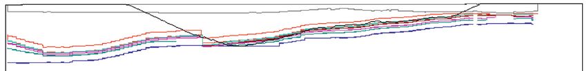
6 Mathematical Problems in Engineering

 Table 1: Technical and economic parameter values used in the DP model.
 Coal mining Rock mining Stripping cost of UCM Mining Cost
Coal price Coal price
 cost cost unconsolidated material recovery escalation Discount rate (%)
(RMB·t−1) escalation (%)
 (RMB·t−1) (RMB·m−3) (RMB·m−3) (%) (%)
250 20 28 18 95 0.0 0.0 7.0

5. Case Study Table 2: Major quantities of the best phase plan.
 Phase 1 Phase 2 Phase 3 Phase 4 Total
A software package has been developed based on the above
model and algorithm and was used in a case study on a large Coal
 200.15 200.50 200.66 220.29 821.60
 quantity/Mt
coal deposit in northern China. The topography of the coal
 Rock
field is nearly flat with a maximum relief of less than 20 m. quantity/Mm3
 640.18 847.81 1012.22 1391.33 3891.54
The surface boundary of the planning area is about 7800 m UCM
long and 4500 m wide. From drill hole information, 8 coal 476.46 320.68 302.97 206.65 1306.76
 quantity/Mm3
seams were identified, with thicknesses varying from around Average strip
 5.58 5.83 6.55 7.25 6.33
1 m to around 40 m and densities between 1.28 and 1.31 t/ ratio/m3:t
m3. The deposit was modeled into a column model having Time length/a 10.01 10.02 10.03 11.01 41.07
around 39000 columns, each having a horizontal cross NPV/M RMB 13716.69 5920.99 2235.72 712.15 22585.55
section of 30m × 30 m. The attributes of each column, mainly
the thickness and elevation of each coal seam along the
column, were estimated based on drill hole data using an ultimate pit. Figure 5 is a vertical cross section of the phase-
inverse distance interpolation method particularly designed pits superimposed on the coal seams in the column model.
for this study. The direction of phase expansion can be clearly seen from
 The coal reserve within the planning boundary was these figures. One can also see the rationality of the opti-
estimated to be some 900 Mt. For a deposit of this scale, mization results from the spatial relationship between the
the annual coal mining rate was assumed to be 20 Mt of phase-pits and the coal seams (Figure 5).
run-of-mine coal. The coal is to be sold without pro- The developed software provides an option of keeping
cessing. The time span of a single phase is generally more and outputting a specified number of best phase plan sce-
than 5 years to avoid complications associated with narios. For the case study, we found five other scenarios with
frequent transitions between phases. Therefore, in gen- virtually the same NPVs as the one given in Table 2, but with
erating the least-SR pits, the coal quantity of the smallest different numbers of phases, and/or phase-pits (including
pit, Q1, was set to 100 Mt (5-year production), and the the ultimate pit). Since it is very difficult, if not impossible, to
coal quantity increment, ΔQ, to 20 Mt. A maximum pit incorporate all relevant practical considerations in any
slope of 25° was used. With these parameter values and optimization model and algorithm, these phase plan sce-
the column model as inputs, 40 nested pits were gen- narios, which are equally good economically, provide
erated by applying the cone eliminating algorithm de- valuable options for further evaluation with respect to
scribed above. The coal quantity increment between any certain practical considerations to arrive at the final phase
two consecutive pits in the generated pit series has a very plan.
small variation (20.00 Mt to 20.17 Mt), indicating that the We also analyzed the effects of certain input pa-
algorithm has produced an evenly spaced series of nested rameters, such as coal price, production costs, and their
pits with increments virtually equal to the specified value. escalation rates, on the phase planning outcome for the
This is a verification of the algorithm’s capability of case study, with the above phase plan as the base case for
completely overcoming the gap problem. comparison. The planning outcome was found to be
 The phase plan was optimized with the generated pit sensitive with respect to these parameters. When the coal
series and the parameter values in Table 1 as inputs to the DP price was lowered by 20%, the size of the optimum ul-
model. The best (highest-NPV) phase plan consists of 4 timate pit decreased by 30%, and the number of phases
phases and Table 2 summarizes the major quantities to be decreased from 4 to 3. Increasing the production costs by
mined in the phases. With an annual coal production of 20% had similar effects. Increasing the coal price (or
20 Mt, each of the first three phases has a time span of 10 lowering the production costs) had reverse effects on the
years and the fourth phase 11 years, giving a total mine life of planning outcome, as expected. Setting the annual es-
41 years. The average strip ratio increases from phase 1 to calation rates of coal price and production costs to 2.0%
phase 4. Since maximizing NPV implies postponing waste and 1.5%, respectively, resulted in a 7% larger ultimate
removal as much as possible, the increasing strip ratio with pit, the same number of phases, but larger phase-pits.
time is a verification of the rationality of the proposed Based on the outcomes of these experiments, we suggest
method. that the phases should be updated periodically (e.g.,
 Figure 4 is a 3D view of the four phase-pits of the op- toward the end of each phase) in a real-life operation, as
timized phase plan, where phase-4 pit is also the best the relevant economic and technical conditions change

Mathematical Problems in Engineering 7

 (a) (b)

 I

 Fault
 I

 (c) (d)

Figure 4: 3D view of the phase-pits of the best phase plan. (a) Phase-1 pit. (d) Phase-4 pit (ultimate pit). (c) Phase-3 pit. (b) Phase-2 pit.

 Phase 3 Phase 2 Phase 1

 Unconsolidated

 Phase 4 Phases 1, 2, 3
 Phase 4 Coal seams

 Figure 5: The phase-pits on a vertical cross section at I–I.

over time. The optimization method presented herein advantage over the commonly used block model in the
and the developed software can be a handy tool for accuracy of coal quantity computation with nearly hor-
updating phase plans. izontal and bedded coal seams. The method is capable of
 handling large real-life instances and produces rational
6. Conclusions results, as demonstrated by the case study. The method
 can also be used to analyze the effects of relevant input
The phase planning method presented herein is specially parameters on the phase planning outcome, providing
designed for open pit coal mines with nearly horizontal useful scenarios for decision-making in strategic plan-
and bedded coal seams. The major merits of the method ning of open pit coal mines.
include the following: it simultaneously optimizes the The proposed method in its current form has two major
number of phases, the intermediate phase-pits, and the shortcomings. One is that the total cost of mining a phase is
ultimate pit; it eliminates the gap problem in generating a averaged over the years of the phase’s time span while, in
series of nested pits; and the column model has a clear actuality, the quantities of rock and unconsolidated material

8 Mathematical Problems in Engineering

mined each year fluctuate within a phase, causing fluctua- Operations Research in the Mineral Industries, pp. 485–494,
tions in annual cost. Another shortcoming concerns the Littleton, CO, USA, January 1989.
transition from one phase to the next. Transition takes place [8] D. Dagdelen and J. T. B. Johnson, “Optimum open pit mine
sometime before a phase is completely mined out. During production scheduling by Lagrangian parameterization,” in
the transition period, the upper benches of the next phase are Proceedings of the 19th International Symposium on the Ap-
 plication of Computers and Operations Research in the Mineral
mined and some working benches may traverse the
 Industries, pp. 127–139, Altoona, PA, USA, January 1986.
boundary between the two phase-pits. Phase transitions are [9] Q. Wang and H. Sevim, “Alternative to parameterization in
not incorporated in our current formulation and should be finding a series of maximum-metal pits for production
dealt with in a more detailed scheduling process. Over- planning,” Mining Engineering, pp. 178–182, 1995.
coming these shortcomings will be the focus of our future [10] C. Meagher, R. Dimitrakopoulos, and V. Vidal, “A new ap-
research on this topic. proach to constrained open pit pushback design using dy-
 namic cut-off grades,” Journal of Mining Science, vol. 50, no. 4,
Data Availability pp. 733–744, 2014.
 [11] P. Goovaerts, Geostatistics for Natural Resources Evaluation,
The data used to support the findings of this study are Oxford University Press, Oxford, UK, 1997.
available from the corresponding author upon request. [12] R. Dimitrakopoulos, “Conditional simulation algorithms for
 modelling orebody uncertainty in open pit optimisation,”
 International Journal of Surface Mining, Reclamation and
Conflicts of Interest Environment, vol. 12, no. 4, pp. 173–179, 1998.
 [13] R. Dimitrakopoulos, C. T. Farrelly, and M. Godoy, “Moving
The authors declare that they have no conflicts of interest. forward from traditional optimization: grade uncertainty and
 risk effects in open-pit design,” Mining Technology, vol. 111,
Acknowledgments no. 1, pp. 82–88, 2002.
 [14] A. Boucher and R. Dimitrakopoulos, “Multivariate block-
The authors acknowledge the National Natural Science support simulation of the yandi iron ore deposit, western
Foundation of China (51674062, 51974060, and 51474049), Australia,” Mathematical Geosciences, vol. 44, no. 4,
National Science Foundation for Young Scientists of China pp. 449–468, 2012.
(51604061), and Liaoning Province Key Research and De- [15] R. Goodfellow and R. Dimitrakopoulos, “Algorithmic inte-
velopment Project (2019JH2/10300051), for their financial gration of geological uncertainty in pushback designs for
supports in the course of the research work presented in this complex multiprocess open pit mines,” Mining Technology,
paper. vol. 122, no. 2, pp. 67–77, 2013.
 [16] M. W. A. Asad and R. Dimitrakopoulos, “Implementing a
 parametric maximum flow algorithm for optimal open pit
References mine design under uncertain supply and demand,” Journal of
 the Operational Research Society, vol. 64, no. 2, pp. 185–197,
 [1] H. Lerchs and I. F. Grossmann, “Optimum design of open-pit 2013.
 mines,” Canadian Mining and Metallurgical Bulletin, vol. 58, [17] M. Asad, “Performance evaluation of a new stochastic net-
 pp. 47–54, 1965. work flow approach to optimal open pit mine design-appli-
 [2] A. G. Journel, “Convex analysis for mine scheduling,” in cation at a gold mine,” Journal of the Southern African
 Advanced Geostatistics in the Mining Industry, Reidel Pub- Institute of Mining and Metallurgy, vol. 112, pp. 649–655,
 lishing Co. Dordercht, Dordercht, Netherlands, 1975. 2012.
 [3] F.-B. Dominique and M. Alain, “New method for open-pit [18] M. W. A. Asad, R. Dimitrakopoulos, and J. V. Eldert, “Sto-
 design: parameterizing of the final pit contour,” in Proceedings chastic production phase design for an open pit mining
 of the 14th International Symposium on Application of complex with multiple processing streams,” Engineering
 Computers and Operations Research in the Mineral Industry, Optimization, vol. 46, no. 8, pp. 1139–1152, 2014.
 pp. 573–583, New York, NY, USA, April 1976. [19] X. Gu, Q. Wang, and S. Ge, “Dynamic phase-mining opti-
 [4] F.-B. Dominique and M. Alain, “Algorithms for parameter- mization in open-pit metal mines,” Transactions of Nonferrous
 izing reserves under different geometrical constraints,” in Metals Society of China, vol. 20, pp. 1974–1980, 2010.
 Proceedings of the 17th Symposium on the Application of
 Computers and Operations Research in the Mineral Industries,
 pp. 297–309, New York, NY, USA, 1982.
 [5] F.-B. Francois-Bongarcon and M. Dominique, “Parameteri-
 zation of optimal designs of an open pit: beginning a new
 phase of research,” Transactions of American Society for
 Mining, Metallurgy, and Exploration, Inc. (SME), vol. 274,
 pp. 1801–1805, 1984.
 [6] D. Dagdelen and F.-B. Kadri, “Towards the complete double
 parameterization of recovered reserves in open pit mining,” in
 Proceedings of the 17th Symposium 17th Symposium on the
 Application of Computers and Operations Research in the
 Mineral Industries, pp. 288–296, New York, NY, USA, 1982.
 [7] C. Thierry, “Technical parameterization of reserves for open
 pit design and mine planning,” in Proceedings of the 21th
 International Symposium on the Application of Computers and