Joint Action Recognition and Pose Estimation From Video
←
→
Page content transcription
If your browser does not render page correctly, please read the page content below
Joint Action Recognition and Pose Estimation From Video
Bruce Xiaohan Nie, Caiming Xiong and Song-Chun Zhu
Center for Vision, Cognition, Learning and Art
University of California, Los Angeles, USA
{niexh,caimingxiong}@ucla.edu, sczhu@stat.ucla.edu
Abstract
Action recognition and pose estimation from video are
closely related tasks for understanding human motion, most
methods, however, learn separate models and combine them
sequentially. In this paper, we propose a framework to in-
tegrate training and testing of the two tasks. A spatial-
temporal And-Or graph model is introduced to represent ac-
tion at three scales. Specifically the action is decomposed
into poses which are further divided to mid-level ST-parts
and then parts. The hierarchical structure of our model
captures the geometric and appearance variations of pose
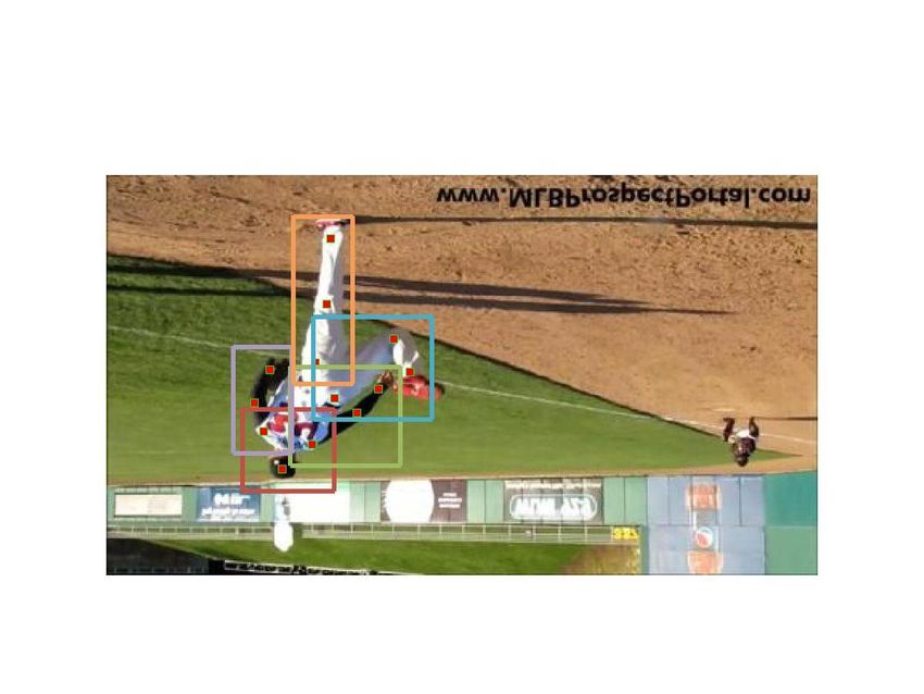
at each frame and lateral connections between ST-parts at Figure 1. (a) Single frame human poses estimated by [29]. (b)
adjacent frames capture the action-specific motion informa- Action recognition and poses estimation by our approach.
tion. The model parameters for three scales are learned dis-
criminatively, and action labels and poses are efficiently in-
ferred by dynamic programming. Experiments demonstrate background in action datasets, the most discriminative parts
that our approach achieves state-of-art accuracy in action (such as ’arms’, ’hands’, ’legs’ and ’feet’) are often missed
recognition while also improving pose estimation. in pose estimation, thereby deteriorating subsequent action
recognition. However, those human parts have large motion
in actions and can be recovered by motion information. For
1. Introduction example, Fig. 1 shows that the arms and legs mis-detected
by a pose estimation method [29] are successfully detected
1.1. Motivation and Objective by our method. Besides the motion information on arms and
Action recognition and pose estimation are both im- legs, action recognition also provides strong priors on the
portant tasks for vision-based human motion understand- pose sequences. Furthermore, if actions are limited to pre-
ing. They are widely used in applications, such as, intel- defined categorizes, the actions provide strong constraints
ligent surveillance systems and human-computer interac- on the plaussible poses in space and time [7].
tion systems. Despite their different goals, the two tasks Many methods for action recognition bypass body poses
are highly coupled and it is desirable to study them in and achieve promising results by using coarse/mid-level
a common framework. However, existing methods train features for action classification on some datasets[6, 10,
models for the two tasks separately and combine the infer- 26, 12, 18, 2, 33, 30]. In this paper, we will jointly train
ence sequentially: taking pose estimation as input for ac- coarse/mid-level features with pose estimation so that these
tion recognition[15, 34, 25, 8, 27, 24]. For certain actions features are better aligned with body parts and improve the
defined by specific geometric configuration of body parts, results.
pose estimation from a single image may be sufficient for The prevailing methods for pose estimation from still im-
action recognition [15, 28, 5, 32]. ages adopt probabilistic and compositional graphical mod-
The main drawback of such methods is that the accu- els where nodes represent part appearance and edges rep-
racy of action recognition highly relies on the obtained pose resent geometrical deformation[29, 19, 17, 20]. Errors
estimations. Due to the large pose variation and complex mainly arise from small parts, like forearms and wrists due
1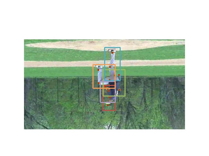
And Node   Or Node   Terminal Node

                                                                                          Coarse-level         Mid-level         Fine-level
                                         Baseball                                                               feature            feature
                                                                                             feature
                                           pitch
 Action                                                        Coarse-level
                                                                  feature

                    Pose 1            Pose 2        Pose 3         Pose T
                                                             ...
 Poses

                                                                        Mid-level                              (b)
                                                                         feature
ST-parts                                                                                 t=1             t=2               t=3          t=T

                                                                                                                                        ...
Parts                                                                       Fine-level
                                                                              feature

                                  (a)                                                                          (c)

Figure 2. (a) Our spatial-temporal AOG model for action ”Baseball pitch”. The action is decomposed into poses, ST-parts, and parts. Each
ST-part is an Or-Node that represents the mixture components. For simplicity we only draw all nodes at the second frame. The orange edges
represent geometric deformations between ST-parts and parts. (b) The three feature levels. Action nodes, ST-part nodes and part nodes
connect to terminal nodes that represent coarse-level, mid-level and fine-level features respectively. (c) An example of temporal relation
on ST-part ’left arm’. The purple edges connecting five ST-parts at adjacent frames capture the temporal co-occurrence and deformation
relations. During inference we select the best component (red rectangle) for each ST-part.

to large variation and blending with background features.                        into poses at each frame. Each pose is decomposed into
Video pose estimation methods capture motion informa-                            five independent mid-level ’ST-parts’ (ST means Spatio-
tion by adding many pairwise terms among parts at sub-                           Temporal) that cover a large portion of human bodies and
sequent frames to the graphical model[3, 36, 21], however,                       are robust to image variations. All fine-level parts are condi-
these models are loopy and require approximate inference.                        tioned on their ST-part parents. Each ST-part is discretized
The smoothness features on pairwise terms are restricted to                      into several components by clustering. The ST-parts with
videos with slow motion and small appearance variation,                          the same component can be seen as a poselet[1] that has
but such prior assumptions break in action datasets. Human                       small variation of appearance and deformation and each
motion can become much larger and the changing of view-                          component is represented by mid-level features and fine-
point makes appearance inconsistent at adjacent frames. As                       level part features from single image pose estimation.
illustrated in Fig. 1, we improve the estimation of part loca-                       In order to capture the specific motion information of
tions by using action specific information.                                      each action, ST-parts at adjacent frames are connected to
                                                                                 represent temporal co-occurrence and deformation. The
1.2. Method Overview                                                             model parameters at three levels are trained separately by
                                                                                 S-SVM and combined by a mixture of experts method. Due
   This paper integrates the training and testing of action
                                                                                 to the independence between ST-parts of each pose, we can
recognition and video pose estimation. During training, in-
                                                                                 infer both action label and poses efficiently by DP.
formation from both tasks is utilized to optimize model pa-
rameters and in testing the action labels and part locations
                                                                                 2. Related Works and Our Contributions
are inferred jointly.
   We start by building a spatial-temporal And-Or graph                             Action recognition and pose estimation are both popular
model[37][23][14][13] to represent actions and poses                             topics in computer vision and there are numerous literature.
jointly. Hierarchical structure of our model can represent                       This section refers to some recent work on both topics. Ac-
top-down part geometric configurations in a single frame                         tion recognition methods are grouped into two categories:
and lateral temporal pose relation in subsequent frames. On                      coarse/mid-level feature based and pose feature based. Pose
the top layer, the low-resolution action information is cap-                     estimation methods are reviewed with two aspects: single
tured by coarse-level features and the action is decomposed                      image pose estimation and video pose estimation.

                                                                            2
Coarse/mid-level feature based methods. The most                 mation. It formulates the pose estimation as an optimization
successful framework is built on spatial-temporal interest           over a set of action specific manifold and conducts the two
points such as cubiods[6] and 3D Harris corner[10]. This             tasks iteratively. In training it requires that each video is
framework extends object detection using 2D spatial inter-           from multiple views however we can work on datasets in
est points. After the interest points are detected, appear-          which each sample is from only one view.
ance and motion features like HOG[4] and HOF[11] are                    This paper combines action recognition and video pose
extracted and the bag-of-words representation is used for            estimation in a unified framework with a spatial-temporal
classification. Instead of using interest points, Wang et al.        And-Or Graph model. This paper makes three contributions
[26] extracts dense trajectories by optical flow and builds a        to both action recognition and video pose estimation prob-
bag-of-words representation on trajectory aligned features.          lems:
While it has achieved good performance on many action                   i) It proposes a spatial-temporal AOG model to integrate
datasets, it highly relies on the quality of optical flow. Al-       action recognition and video pose estimation. The two tasks
though the coarse/mid-level features based methods suc-              are mutually benefit from each other in training and testing.
ceed on some datasets, they offer no intuition about the re-            ii) It represents actions at three scales. Coarse and mid-
lation between pose and action. The learning and inference           dle level features are trained jointly with pose features.
with these methods is simple and fast, and they can work on             iii) It outperforms state-of-art action recognition and
the low-resolution videos.                                           pose estimation methods on two action datasets: Penn Ac-
    Pose feature based methods. Recently, due to the great           tion dataset and sub-JHMDB dataset.
progress made in pose estimation, many action recognition
methods try to borrow strength from high-level pose infor-           3. Representation and Modeling
mation. Yao et al. [34] represents action as several key-            3.1. Spatial-Temporal And-Or Graph Model
poses with an AOG model. Each key pose corresponds
to a latent variable in a HMM model. Wang et al. [25]                   Fig.2 shows our spatial-temporal AOG model for repre-
first runs pose estimation on video frames and builds pose           senting action and poses. There are three kinds of nodes:
features directly on the estimated poses, classifying with a         And nodes, Or nodes and Terminal nodes. The And node
bag-of-words framework. Jiang Wang et al. [27] develops              captures the decomposition of a large entity. In our case the
MST-AOG model for cross-view action recognition. The                 action and poses are represented by And nodes because they
3D skeleton training data is applied to help mine the dis-           are decomposed into several children. The Or node repre-
criminative parts.                                                   sents structural variations. Here each ST-part is an Or node
    Single image pose estimation methods. The most pop-              because it has different components. The Terminal node is
ular framework used in single image pose estimation is to            observable and directly associates with image evidence. We
build a part graphical model based on human joints. Yang             have three kinds of terminal nodes to represent actions at
and Ramanan [29] build a tree-structure spring model to              different scales. The terminal nodes associated with action
capture both spatial and co-occurrence relations between             and ST-parts represent coarse and mid-level features and the
parts. Brandon et al. [19] uses a compositional AOG model            terminal nodes at bottom level represent fine part features.
to represent large appearance and geometry variation and                To unify action recognition and video pose estimation
image segmentation is employed to help distinguish the               each action example A is represented by the poses pt at each
parts from cluttered background. Pishchulin et al. [17]              frame:
builds a more flexible graphical model with strong local                                  A = {p1 , p2 , ..., pT }             (1)
appearance representations and the mid-level semi-global                T is the number of frames. Each pose pt is represented
poselets are combined with fine part appearance model.               by an And node and decomposed into several ST-parts li
    Video pose estimation methods. Cherian et al. [3]                (Fig. 2(a)):
extends the graphical model with temporal edges between                                 pt = {l1 , l2 , ..., lM }          (2)
parts at adjacent frames. The geometric and appearance
                                                                       M is the number of ST-parts. Each ST-part li is a mixture
comparability between parts is captured by temporal edges
                                                                     components model with several parts oj :
and approximate inference is performed on the highly loopy
graphical model. Instead of using a graphical model Shen et                             li = {o0 , ..., oNi −1 , ci }            (3)
al. [22] formulates the video pose estimation as a matching
problem that tries to match the dense trajectories from 2D               oj = {xj , yj } denotes the position of part j which
video with the projection of the 3D trajectories of human            should be one of the human joints, oj ∈ Ωpart , Ωpart =
motion under different viewpoints in a 3D database.                  {0 head0 ,0 torso0 ,0 lef tarm0 ,0 rightarm0 , ...}, Ni is the
    To the best of our knowledge Yao et al. [31] is the only         number of parts that belong to parent i, o0 is the root part for
paper that tries to couple action recognition and pose esti-         this ST-part. ci is the component id and ci ∈ {1, 2, ..., zi },

                                                                 3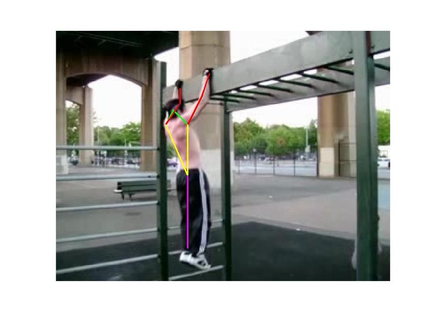
zi is the number of components of ST-part i. The ST-parts                  The score of ST-part i is defined by:
with the same component have small appearance and geo-                                                      Ni                     Ni
metrical variations and represent a motion status of the ac-             S(li ) = Sd (li ) + Sh (li ) + λ
                                                                                                            X
                                                                                                                  S(oj ) + λ
                                                                                                                                   X
                                                                                                                                         S(oj , o0 )
tion. The learning of ST-parts will be discussed in the next                                                j=0                    j=1
section.                                                                                                                             (4)
    We divide the feature vector of ST-part into two cate-                  There are four terms contributing to the ST-part score.
gories: classification feature for action classification and            The first two terms are classification scores and the last
detection feature for regularization.                                   two terms are detection scores. Sd (li ) =< ωdli , ψ(li ) >
    Classification feature includes two terms: ψ(li ) and               measures the compatibility of component ci . Sh (li ) =<
ψ(ci ). ψ(li ) = [d1 d2 ... dzi ]T where dj = (o0 − uj ) is the         ωhli , ψ(ci ) > is the histogram score of component ci . S(oj )
normalized Euclidean distance between the root part and                 is the score of part j and S(oj ) = P (oj ) where P (oj ) is the
the component center. ψ(ci ) = [0, 0, 1(ci ), ..., 0, 0] is a zi        part marginal score from pose estimation. S(oj , o0 ) =<
dimension indicator where the entry corresponding to com-               ω ij , ψ(Edij ) > is the deformation score of part j related to
ponent ci is one and the others are zero.                               the root part. Parameter λ is the weight for detection score.
PNDetection
     i
                 feature contains two portions:
                                              PN the part score
                                                   i
                                                                        The inference algorithm will search all possible ST-parts in
   j=0  S(o  j ) and the    deformation score    j=1 S(oj , o0 ).       the feature pyramid and output a top candidate list for each
The two scores are directly obtained from a single image                frame.
pose estimation[29] and used to regularize action classifica-               Each pose is composed of M ST-parts thus the score is
tion.                                                                   written as a summation of their scores.
    There are two kinds of edges in our model: orange edges                                               M
represent the geometric deformation in a single frame and                                      S(pt ) =
                                                                                                          X
                                                                                                                  S(lit )                        (5)
purple edges represent the smoothness and temporal co-                                                      i=1
occurrence of ST-parts at adjacent frames.
    Deformation feature is a four-dimension vector which                   The relation between ST-parts in a single image is ig-
models deformation between ST-part and part as a 2D gaus-               nored so they are independent of each other, avoiding the
sian distribution: ψ(Ed ) = [dx, dy, dx2 , dy 2 ]T , Ed ∈ ΩD .          loopy graph structure that is a common case in video pose
    Temporal co-occurrence feature at ST-part i of                      estimation. The details will be discussed in section 5.
frame t is a zi × zi dimension indicator: ψ(Eo ) =                         In our model, each action example is a sequence of poses
[0, 0, 1(ct )1(ct+1 ), ..., 0], Eo ∈ ΩO which means that only           following the transitions between poses at adjacent frames.
the entry corresponding to components ct and ct+1 is one                Thus, the fine-level score of an action can be formulated as:
and the others are zero.                                                                       T
                                                                                               X                  T
                                                                                                                  X −1
    Smoothness feature d(lit , lit+1 ) is the negative Eu-                         SH (A) =          S(pt ) +            S(pt+1 |pt )            (6)
clidean distance between the root parts of lit and lit+1 .                                     t=1                t=1

    Although the action is represented by a sequence of                     S(pt ) is defined in Eq. (5) and S(pt+1 |pt ) measures
poses, it is insufficient to only use pose features for action          the transition score between two poses. The transition re-
recognition because low resolutions makes part detection                lation of two poses is captured by transitions between their
unreliable. Here we borrow the strength from coarse-level               ST-parts and it is thus written as a summation of transition
and mid-level features for compensation. For the coarse                 scores of ST-parts.
feature ψL , we follow the framework of [26] to extract the
                                                                                                            M
bag-of-words feature on the dense trajectories. For the mid-                                                X
                                                                                        S(pt+1 |pt ) =            S(lit+1 |lit )                 (7)
level feature ψM , we use the method from [27] to train
                                                                                                            i=1
HOG/HOF templates for each selected ST-part component,
using the filter responses as features.                                    The transition score between two ST-parts is defined as:

3.2. Score Functions                                                              S(lit+1 |lit ) = S(cti , ct+1
                                                                                                            i   ) + βd(lit , lit+1 )             (8)

    In this section, we introduce the score functions of our               It includes two components: the co-occurrence score
                                                                                                      ct ,ct+1
model in a bottom-up fashion. For simplicity we drop the                S(cti , ct+1
                                                                                 i   ) =< ωoli , ψ(Eoi i ) > and smoothness score
action label in all formulations in this section.                             t t+1
                                                                        βd(li , li ), where β is the weight for the smoothness.
    The terminal nodes in the bottom layer ground all parts                The fine-level score of one image sequence is rewritten
to image data. Instead of training part templates with action,          as follows, combining eqns. (5), (6) and (7).
we train them independently by single image pose estima-                                     M X T           T −1
tion [29]. The part scores and part deformation scores are
                                                                                             X               X
                                                                                SH (A) =       (   S(lit ) +      S(lit+1 |lit ))                (9)
obtained directly from [29].                                                                 i=1 t=1                 t=1

                                                                    4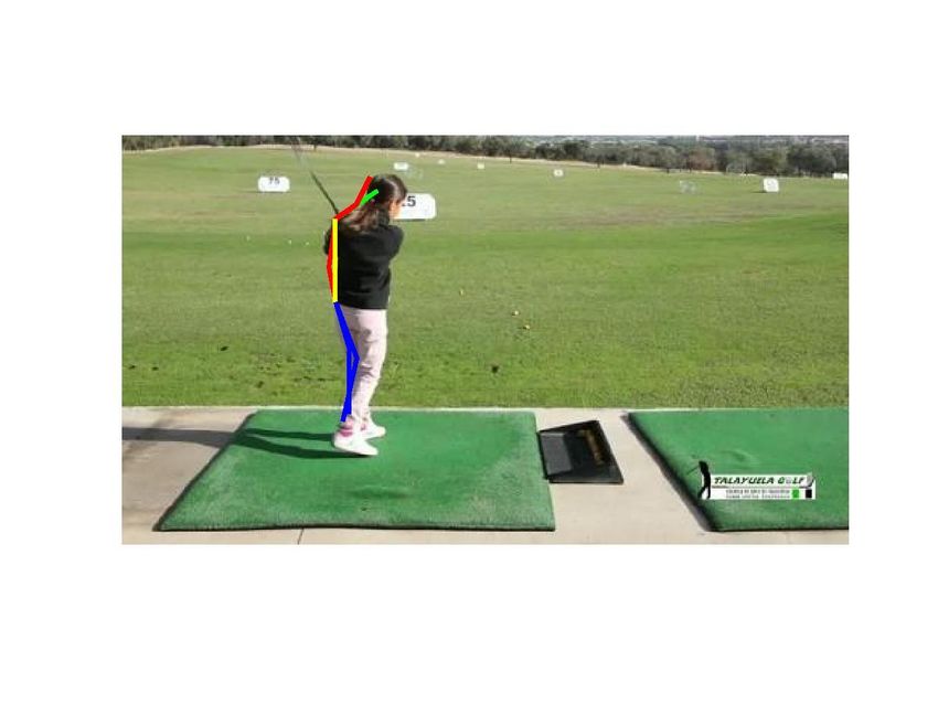
In this form, the fine-level score is only related to the ST-                        shared by two ST-parts and we pick them from the ST-part
parts. The inference algorithm will search for the positions                            ’head shoulder’ because it is more robust than ’left arm’ and
and components of ST-parts that maximize this score.                                    ’right arm’.
   With coarse-level and mid-level scores, the action score                                 To speed up computation, we first run [16] for each
can be written as,                                                                      frame and compute response maps for all ST-parts. After
 S(A) = πL (A)SL (A) + πM (A)SM (A) + πH (A)SH (A)                                      non-maximum suppression we pick the ST-part candidates
                                                           (10)                         that have a score above τ . We connect all candidates on con-
SL (A) =< ωL , ψL (A) > is coarse-level score and                                       secutive frames and compute their unary scores and binary
SM (A) =< ωM , ψM (A) > is mid-level score. The                                         transition scores. To determine the optimal threshold τ , we
weights πL (A) =< ωL         0
                               , φ0L (A) >, πM (A) =<                                   compute ST-part scores on the ground truth of all training
ωM0
    , φ0M (A) > and πH (A) =< ωH       0
                                         , φ0H (A) > are linear                         images and pick the highest value for the threshold that does
functions on features of action example A.                                              not prune the optimal one on training examples.

4. Inference                                                                            5. Learning

                 t=2
                                                                                           Our learning process includes two main stages: The first
    t=1                        t=3
                                                                                        stage is to learn ST-parts. The second stage is to learn
                                                                                        the model parameters for three levels including weights for
                                                                                        unary ST-part score , temporal score between ST-parts in
                                                                                        adjacent frames and classification weights for each action.

                                                                                        5.1. Learning ST-parts
                                                                                            As a mid-level representation of human pose, ST-parts
    1             1             1                                                       are much more robust to image variations than fine parts,
                                                                                        especially on action datasets containing large appearance,
    2             2             2
                                                                                        geometric and motion variations that make fine parts hard
    3             3             3                                                       to detect. With pose annotations we can learn ST-parts from
                                                                                        training data.
                 (a)                                         (b)
Figure 3. An example of our inference method. (a) For each frame
we generate several ST-part candidates and obtain the best path for                     5.1.1   ST-part Representation
each ST-part by DP. (b) The ST-part is represented by the mid-level
features (HOG and HOF template) and fine-level features (scores                         We use 13 joints to represent the human subject. The
of knee and ankle).                                                                     13 joints are divided into 5 ST-parts: ’head-shoulder’,’left
                                                                                        arm’,’right arm’,’left leg’,’right leg’ each of which includes
   The objective of our inference is to find the action la-                             3 joints Fig.5(a). In order to compute deformation we de-
bel and part locations. The coarse-level score SL (A) and                               fine 5 joints as root parts for ST-parts:head, left elbow, right
mid-level score SM (A) are computed directly by linear-                                 elbow, left knee, right knee. Each ST-part is encoded by a
SVM. As illustrated in Fig.3 (a), The fine-level action score                           feature vector:
SH (A) is divided into M independent terms each of which
corresponds to the summation of unary scores and binary                                             f (lit ) = [∆p1 , ∆p2 , ∆pt0 , ∆pt1 , ∆pt2 ]      (12)
transition scores for one ST-part, thus dynamic program-
ming can be used to find the best ST-part path:
                                                                                            ∆p1 = p1 − p0 and ∆p2 = p2 − p0 are the offsets of
                                     T
                                     X                 T
                                                       X −1                             parts relative to the root part. ∆pt0 = [pt−1
                                                                                                                                   0   − pt0 , pt+1
                                                                                                                                                0   − pt0 ]
 [li1 , li2 , ..., liT ] = arg max         S(lit ) +          S(lit+1 |lit ) (11)       is the temporal offset of root part relative to the same joint
                                     t=1               t=1                              in previous frame and the next frame. ∆pt1 and ∆pt2 are
   This procedure is repeated M times to find the total M                               defined in the same way. Using the temporal offset as a
best paths for each action label. Finally the action label                              feature is important because some ST-parts have the same
with maximum score is obtained in Eq. (10).                                             joint configuration and can be only distinguished by motion.
   With the best action label, we trace back to the best ST-                            To make the feature invariant to scale, we estimate the pose
part paths for the action and obtain all joint locations. No-                           scale st at each frame by head length, and then the feature
tice that the joints ’left shoulder’ and ’right shoulder’ are                           is normalized by the scale factor: f (lit ) = f (lit )/st .

                                                                                    5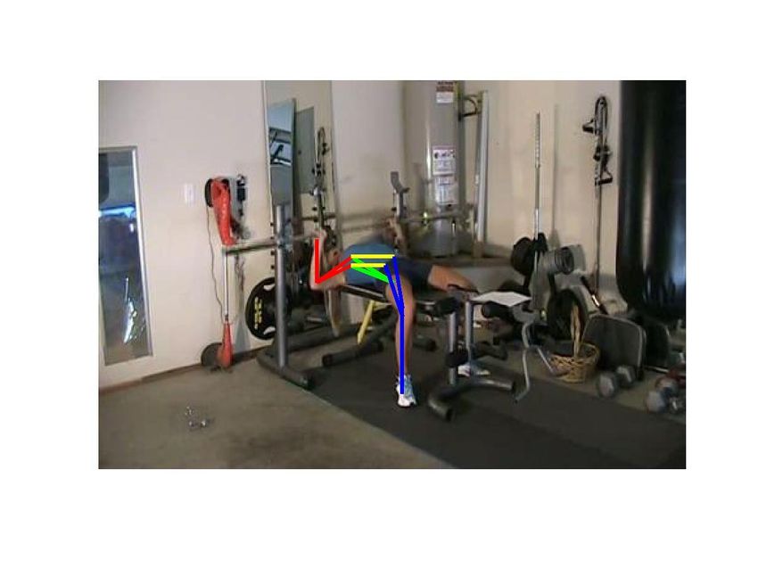
(a)                                   (b)                                                  (c)
Figure 4. (a) The 13 joints used in our model. They are divided into five ST-parts each of which contains 3 joints. (b) Some examples of
pose annotations in training data and their generated ST-parts. (c) Some examples of two components for each ST-part.

5.1.2   ST-part Clustering                                             parameters with regularization. Although all training data
                                                                       have part annotations and we have ground truth for part lo-
To capture image variations from different viewpoints and              cations and ST-part components, only using ground truth
actions each ST-part is represented as a mixture of com-               may hurt performance because there is a large difference be-
ponents model and the components are obtained by doing                 tween pose estimation results and ground truth in such chal-
k-means on the features f (lit ). In order to make the ST-part         lenging action datasets. Thus we allow the parts to move
component compact in appearance and motion, we first run               between the top N detected parts that are within a certain
k-means on the training examples with same action label                distance of the ground truth part locations. Learning iter-
and view label to get many small clusters each of which has            ates between two steps until convergence:
small variation. Clusters that have few examples and belong                i) To train parameters w = [ωdl1 ωhl1 ωol1 ...ωdlM ωhlM ωolM ],
to only one video are removed as annotation errors. Finally                                                         PNi
                                                                       we discard the detection scores λ j=0                 S(oj ) and
we combine these clusters according to their distance to let             PNi
them to be shared by different actions and viewpoints. See             λ j=1     S(oj , o0 ) and the smoothness score βd(lit , lit+1 )
some examples in Fig.5 (c).                                            and train the parameters with detected poses hi . For the first
                                                                       iteration, h0 is set to ground truth poses. This is formulated
5.2. Learning Model Parameters                                         as a supervised multi-class classification problem:
                                                                                                                Pn
5.2.1   Learning Coarse-level and Mid-level Templates                                       minωt 12 kωt k2 + C
                                                                                                              n    i=1 ξi ,             (13)
                                                                       s.t. maxŷ∈Y ωtT (φ(xi , yit ) − φ(xi , ŷit )) ≥ ∆(yi , ŷi ) − ξi ,
The coarse-level template ωL is learned by linear-SVM on
the dense trajectory features[26]. These features don’t need           Here yit = (ai , hti ) where ai is action label. ∆(yi , ŷi ) is 1 if
any pose information and they capture the appearance and               ai = âi and 0 otherwise. t indexes the iteration.
short-term motion on the moving blocks. The mid-level in-                  ii) After computing parameters at iteration t, we add the
formation is captured by HOG/HOF templates of ST-parts.                detection score and the smoothness score back into the fine-
Following[27], we train HOG/HOF templates on our ST-                   level score function and infer the poses for each training
part components with SVM and convolute them with train-                example. λ and β are determined by experiments. Similar
ing images. The feature vector is constructed by performing            to inference in testing, we first generate the top N ST-parts
spatial-temporal max-pooling on response maps, and the                 candidates within a certain distance around the ground truth
template ωM is learned by linear-SVM.                                  and find the best ST-part paths among those candidates un-
                                                                       der the ground truth action label by Eq. (11). Then we get
5.2.2   Learning Fine-level Parameters                                 the poses ht+1
                                                                                    i   from the poselets and go back to step 1.
                                                                           After learning the parameters for the three levels, we ob-
The parameters we need to learn for the fine-level score in-           tain the scores for the three levels separately. Finally we
clude ωdli and ωhli for the compatibility score and histogram          learn the weights πL (A), πM (A) and πH (A) to combine
score of each ST-part, ωoli for the ST-part co-occurrence              them for the final action score. We formulate this combi-
score. We adapt latent Structure-SVM for learning those                nation in the mixture of experts framework[9] where each

                                                                   6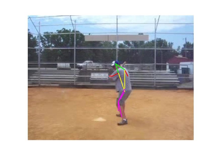
expert corresponds to a classifier in each level. The weights                                 Method                          Accuracy
are computed on each action example, so different weights                                    STIP[35]                           82.9%
indicate which expert the example prefers to use. Here we                                   Dense[26]                           73.4%
concatenate scores of different categories at each level as                                  MST[27]                            74.0%
features to learn the weights.                                                            Action Bank[35]                       83.9%
                                                                                           Actemes[35]                          79.4%
6. Experiments                                                                               Ours(fine)                         73.4%
                                                                                             Ours(all)                          85.5%
    We test our method on two public action datasets: the
Penn Action dataset[35] and the sub-JHMDB dataset[8].                 Table 2. Recognition accuracy on Penn Action dataset. Action
Both datasets are proposed for the purpose of action recog-           Bank is not directly comparable since it uses other training dataset.
nition but they also provide annotations of human joints
which are required by our training approach. The perfor-
mance of both action recognition and pose estimation are              make part detection unreliable and not good enough to clas-
evaluated on each dataset.                                            sify actions.
                                                                         The confusion matrix of Ours(all) is shown in Figure. 6.
6.1. Evaluation on Penn Action Dataset                                Our approach performs well on the actions such as ’bowl’,
    The Penn Action Dataset contains 15 action categories             ’pull up’, ’push up’ and ’squat’, however we achieve low ac-
and the annotations include action labels, rough view la-             curacy on actions with fast movement such as ’tennis fore-
bels and 13 human joints for each image. The occlusion                hand’ because the motion blur makes the positions of criti-
label of each joint is also provided. We follow [35] to split         cal parts like wrists always wrong.
the data into 50/50 for training/testing. The action ’playing
guitar’ and several other videos are removed because less               baseball pitch   .93                                                             .02 .05
than one third of a person is visible in those data. We find           baseball swing    .05 .91                                                         .02 .03

that there exist some un-annotated joints that always remain              bench press              .55                             .02 .08         .33      .02

at the left-top corner of image. To correct those errors we                      bowl                    1.0
                                                                        clean and jerk                         .89 .06                             .06
train a regression model to predict positions of un-annotated
                                                                            golf swing                            .98                                       .02
joints by using the visible neighbor joints from videos with
                                                                            jump rope                                    .89 .11
the same action and view label. In order to get diverse poses
                                                                        jumping jacks                                        1.0
to train [29] we first cluster the training data based on whole
                                                                                pullup                   .03      .03              .94
pose features to get 500 clusters. Then we uniformly select                                    .02 .02                             .02 .93         .02
                                                                              pushup
total 5000 images from those clusters as training images.                        situp   .07 .13         .07                                 .73
We use the code provided by [29], and we set part mixture                       squat                                              .02 .02         .96
number to 8: 6 for visible joints and 2 for occluded joints.           tennis forehand   .08 .10         .07      .03                                    .30 .42
    The number of mixture components of 5 S-T parts are                   tennis serve   .15            .01  .03             .03     .77
43, 37, 31, 56, 58. We find that more components does not                                ba ba be bo cle go jum jum pu pu sit sq ten ten
                                                                                           se se nc wl an lf s p p llu sh up ua ni ni
                                                                                             ba ba h p        an win rop ing p up t  sf ss
improve performance but greatly increase training burden.                                      ll p ll s re
                                                                                                   itc wi ss     d j g e jac
                                                                                                                    er         ks
                                                                                                                                       or er
                                                                                                                                         eh ve
                                                                                                      h ng             k                   an
The parameters λ = 10 and β = 0.01 for detection score                                                                                        d

and smooth score are determined by cross-validation on the            Figure 6. The confusion matrix of our method on Penn Action
training data. Training converges in only 3 iterations. The           Dataset.
coarse-level and mid-level action templates are trained by
the code from [26] and [27]. The number of candidates of                 We compare pose estimation accuracy with Yang et al.
the ST-part ’head-shoulder’ is around 200 and of other ST-            [29] and Park et al. [16]. We use their evaluation criteria
parts is around 1000 because the parts ’head’ and ’shoulder’          and set the threshold to 0.2. The results are illustrated in
only have high scores on a few locations whereas other parts          Table. 1. Our method outperforms theirs at every part. It is
have much larger variations on the score map.                         reasonable that the action specific motion information can
    Table.2 compares the action recognition accuracy be-              help our method to select better parts which are not always
tween previous methods and ours. We use the num-                      the oen with highest score provided by single image based
bers of STIP, Dense, Action Bank and Actemes from                     pose estimation.
[35]. Ours(fine) is trained by only fine-level features and
                                                                      6.2. Evaluation on sub-JHMDB Dataset
Ours(all) is trained with all feature levels. With only fine-
level features, the performance is not very good, but when               The sub-JHMDB dataset contains 316 clips with 12 ac-
coarse/mid-level features are added in the performance is             tion categories. It provides action labels, rough-view labels
improved due to the low resolution and heavy occlusion that           and 15 human joints for each frame. All joints are inside

                                                                  7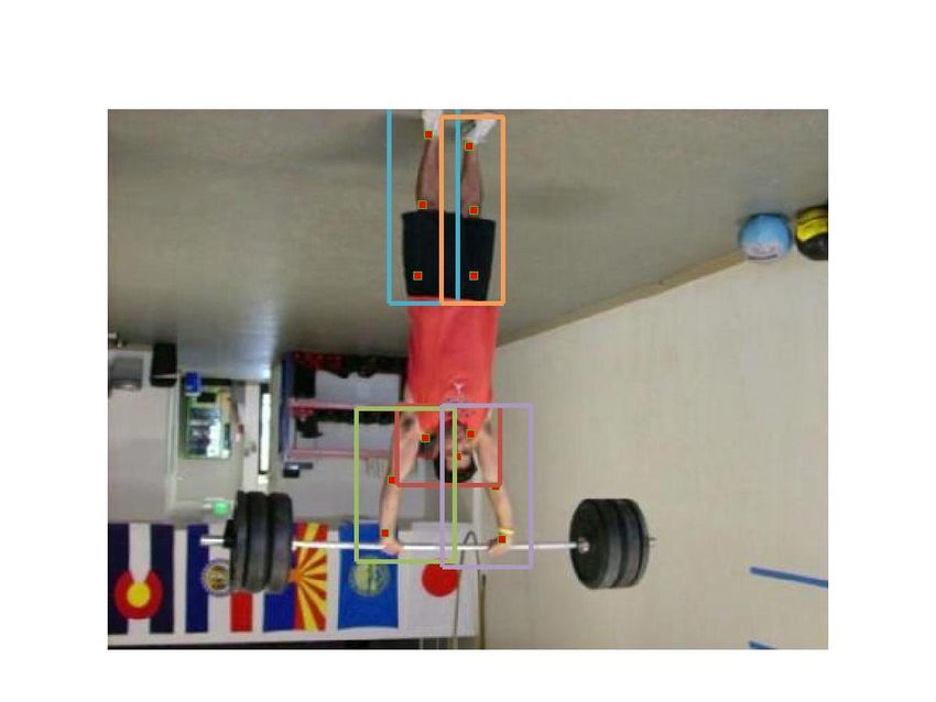
Penn Action Dataset                                                sub-JHMDB Dataset
          Head   Shou    Elbo     Wris     Hip      Knee   Ankle   mean      Head   Shou    Elbo      Wris  Hip      Knee   Ankle   mean
  [29]    57.9   51.3    30.1     21.4     52.6     49.7   46.2    44.2      73.8   57.5    30.7     22.1   69.9     58.2   48.9    51.6
  [16]    62.8   52.0    32.3     23.3     53.3     50.2   43.0    45.3      79.0   60.3    28.7      16.0  74.8     59.2   49.3    52.5
   [3]     −      −       −        −        −        −      −       −        47.4   18.2    0.08      0.07   −        −      −      16.4
  Ours    64.2   55.4    33.8     24.4    56.4      54.1   48.0    48.0      80.3   63.5    32.5      21.6 76.3      62.7   53.1    55.7

Table 1. Pose estimation accuracy in %. The left table shows the results of Penn Action Dataset and the right table shows the results of
sub-JHMDB Dataset.

                 Penn

         sub-JHMDB

Figure 5. Some pose estimation results of our method on the two datasets. The last two columns show failure examples with red rectangle.

the image and there are no un-annotated joints. We use 13                 increased by nearly 6 percent because there are many low-
human joints to train the single image pose estimation. We                resolution videos with large errors of pose estimation.
also do clustering on all frames using the whole pose fea-                   The comparison of pose estimation is illustrated in Ta-
tures and select a total 1500 images from clusters for train-             ble. 1. Our method outperforms [29] the most at parts
ing. The part mixture number is set to 6.                                 ’Head’ and ’Hip’ by nearly 7%, however for the parts ’El-
   We use the 3-fold cross validation setting provided by                 bows’ and ’Wrists’ our performance is comparable which
the dataset to do experiments. The number of mixture com-                 we believe is caused by those parts that are very subtle and
ponents of 5 ST parts are 36, 42, 39, 64 and 64. The param-               because the specific action motion information may prefer
eters λ = 20 and β = 0.01 for detection score and smooth                  the distinguished part locations which are never in the right
score are decided by cross-validation and the training con-               positions. To compare with [3], we re-train their method on
verges in 3 iterations.                                                   our dataset, and they only estimate the joints in upper body.
                                                                          Results show that the pairwise smoothness features they use
                    Method         Accuracy                               are not working well in the action dataset with large motion
                   Dense[8]          46.0%                                and appearance changing.
                   MST[27]           45.3%
                    Pose[8]          52.9%                                7. Conclusion
                   Ours(fine)        55.7%
                   Ours(all)         61.2%                                    We have proposed a new framework to joint action
                                                                          recognition and pose estimation, which are traditionally
     Table 3. Recognition accuracy on sub-JHMDB dataset.                  trained separately and combined sequentially. One limi-
                                                                          tation of our method is that we do not handle the self-
   Table. 3 compares our action recognition performance                   occlusion explicitly which always appears in action datasets
with others. We use the numbers of ’Dense’ and ’Pose’                     and is a big challenge for pose estimation. In the future, we
from [8]. For Pose[8], we use the highest number they ob-                 are going to integrate the 3D pose estimation with the cur-
tained by using pose features extracted from pose estima-                 rent framework, because only with the help of 3D informa-
tion. With only fine-level features our method already out-               tion we can solve the occlusion issue.
performs others. With coarse/mid features the accuracy is                     Acknowledgement: This work is supported by three

                                                                    8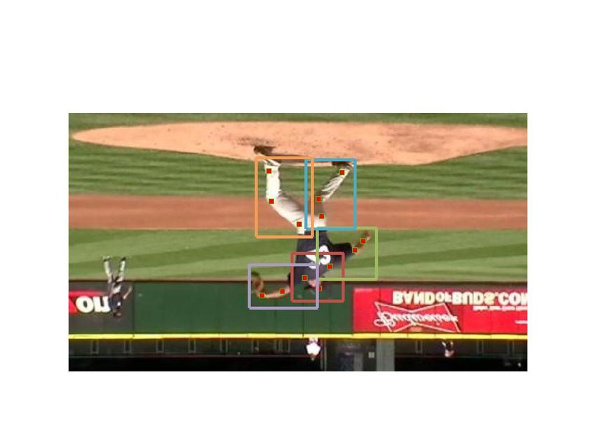
grants: DARPA MSEE FA 8650-11-1-7149, ONR MURI                           [22] H. Shen, S. Yu, D. Meng, and A. Hauptmann. Unsupervised
N00014-10-1-0933, and NSF IIS-1423305.                                        video adaptation for parsing human motion. In ECCV, 2014.
                                                                         [23] X. Song, T. Wu, Y. Jia, and S. C. Zhu. Discriminatively
References                                                                    trained and-or tree models for object detection. In CVPR,
                                                                              2013.
 [1] L. Bourdev and J. Malik. Poselets: Body Part Detectors              [24] Y. Tian, R. Sukthankar, and M. Shah. Spatiotemporal de-
     Trained Using 3D Human Pose Annotations. In ICCV, 2009.                  formable part models for action detection. In ICCV, 2013.
 [2] W. Chen, C. Xiong, and J. J. Corso. Actionness ranking with         [25] C. Wang, Y. Wang, and A. Yuille. An Approach to Pose-
     lattice conditional ordinal random fields. In CVPR, 2014.                Based Action Recognition. In CVPR, 2013.
 [3] A. Cherian, J. Mairal, K. Alahari, and C. Schmid. Mixing            [26] H. Wang, A. Klaser, C. Schmid, and C. Liu. Dense trajecto-
     Body-Part Sequences for Human Pose Estimation. In CVPR,                  ries and motion boundary descriptors for action recognition.
     2014.                                                                    IJCV, 103(1):60–79, 2013.
 [4] N. Dalal and B. Triggs. Histograms of Oriented Gradients            [27] J. Wang, B. X. Nie, Y. Xia, Y. Wu, and S. C. Zhu. Cross-
     for Human Detection. In CVPR, 2005.                                      view Action Modeling, Learning and Recognition. In CVPR,
 [5] V. Delaitre, J. Sivic, and I. Laptev. Learning person-object             2014.
     interactions for action recognition in still images. In NIPS,       [28] W. Yang, Y. Wang, and G. Mori. Recognizing Human Ac-
     2011.                                                                    tions from Still Images with Latent Poses. In CVPR, 2010.
 [6] P. Dollar, V. Rabaud, G. Cottrell, and S. Belongie. Behavior        [29] Y. Yang and D. Ramanan. Articulated human detection with
     Recognition via Sparse Spatio-Temporal Features. In ICCV                 flexible mixtures of parts. PAMI, 35(12):2878–2890, 2012.
     VS-PETS, 2005.
                                                                         [30] Y. Yang, I. Saleemi, and M. Shah. Discovering motion
 [7] J. Gall, A. Yao, and L. Gool. 2D Action Recognition Serves               primitives for unsupervised grouping and one-shote learn-
     3D Human Pose Estimation. In ECCV, 2010.                                 ing of human actions, gestures, and expressions. PAMI,
 [8] H. Jhuang, J. Gall, S. Zuffi, C. Schmid, and M. J. Black.                35(7):1635–1648, 2013.
     Towards understanding action recognition. In ICCV, 2013.            [31] A. Yao, J. Gall, and L. Gool. Coupled action recognition and
 [9] M. I. Jordan and R. A. Jacobs. Hierarchical mixtures of ex-              pose estimation from multiple views. IJCV, 100(1):16–37,
     perts and the EM algorithm. In IJCNN, 1993.                              2012.
[10] I. Laptev and R. Cedex. On space-time interest points. IJCV,        [32] B. Yao and F. F. Li. Recognizing human actions in still im-
     64(2-3):107–123, 2005.                                                   ages by modeling the mutual context of objects and human
[11] I. Laptev, M. Marszalek, C. Schmid, and B. Rozenfeld.                    poses. PAMI, 34(9):1691–1703, 2012.
     Learning realistic human actions from movies. In CVPR,              [33] B. Yao and S. C. Zhu. Learning deformable action templates
     2008.                                                                    from cluttered videos. In ICCV, 2009.
[12] Q. V. Le, J. Ngiam, A. Coates, A. Lahiri, B. Prochnow, and          [34] B. Z. Yao, B. X. Nie, Z. Liu, and S. C. Zhu. Animated pose
     A. Y. Ng. Learning hierarchical spatio-temporal features for             templates for modeling and detecting human actions. PAMI,
     action recognition with independent subspace analysis. In                36(3):436–452, 2013.
     CVPR, 2011.
                                                                         [35] W. Zhang, M. Zhu, and K. Derpanis. From Actemes to Ac-
[13] B. Li, W. Hu, T. Wu, and S. C. Zhu. Modeling occlusion by                tion: A Strongly-supervised Representation for Detailed Ac-
     discriminative and-or structures. In ICCV, 2013.                         tion Understanding. In ICCV, 2013.
[14] B. Li, T. Wu, and S. C. Zhu. Integrating context and oc-            [36] F. Zhou and F. D. Torre. Spatio-temporal Matching for Hu-
     clusion for car detection by hierarchical and-or model. In               man Detection in Video. In ECCV, 2014.
     ECCV, 2014.
                                                                         [37] S. C. Zhu and D. Mumford. A stochastic grammar of images.
[15] S. Maji, L. Bourdev, and J. Malik. Action Recognition from
                                                                              Foundations on Trends in Computer Graphics and Vision,
     a Distributed Representation of Pose and Appearance. In
                                                                              2(4):259–362, 2006.
     CVPR, 2011.
[16] D. Park and D. Ramanan. N-best maximal decoders for part
     models. In ICCV, 2011.
[17] L. Pishchulin, M. Andriluka, P. Gehler, and B. Schiele.
     Strong Appearance and Expressive Spatial Models for Hu-
     man Pose Estimation. In ICCV, 2013.
[18] M. Raptis, L. Kokkinos, and S. Soatto. Discovering Discrim-
     inative Action Parts from Mid-Level Video Representations.
     In CVPR, 2012.
[19] B. Rothrock, S. Park, and S. Zhu. Discriminative Pose Esti-
     mation using Grammar and Segmentation. In CVPR, 2013.
[20] B. Sapp and B. Taskar. Modec: Multimodal decomposable
     models for human pose estimation. In CVPR, 2013.
[21] B. Sapp, D. Weiss, and B. Taskar. Parsing human motion
     with stretchable models. In CVPR, 2011.

                                                                     9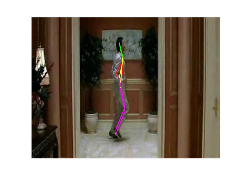
You can also read