The minimum wage and firm networks - Evidence from South Africa WIDER Working Paper 2021/100
←
→
Page content transcription
If your browser does not render page correctly, please read the page content below
WIDER Working Paper 2021/100

The minimum wage and firm networks

Evidence from South Africa

Brandon Joel Tan*

June 2021

Abstract: There is a large literature on the minimum wage focused on directly exposed firms and
geographies. This paper provides new evidence that the minimum wage has significant spillover
effects on firms exposed to the minimum wage indirectly via firm supply chains. Using
administrative firm-level tax data from South Africa, we study the impact of the 50 per cent
agricultural minimum wage hike in 2013 on the outcomes of firms downstream from the
agriculture sector with an event study design. The minimum wage increased labour costs and
prices in the agriculture sector. We find that industries with greater upstream exposure to the
agriculture sector experienced greater decreases in assets, sales, and employment for medium to
large firms following the minimum wage increase.
Key words: minimum wage, supply chains
JEL classification: J23, J31, J46
Acknowledgements: We thank Pol Antras, Emily Breza, Edward Glaeser, Nathan Hendren,
Anders Jensen, Lawrence Katz, Gabriel Kreindler, Michael Kremer, Marc Melitz, and a number
of other colleagues and conference and seminar participants for helpful comments and
suggestions. Responsibility for results, opinions, and errors is the author’s alone.

* Harvard University, Cambridge, MA, USA; btan@g.harvard.edu
This study has been prepared within the UNU-WIDER project Southern Africa—Towards Inclusive Economic Development
(SA-TIED).
Copyright © UNU-WIDER 2021
UNU-WIDER employs a fair use policy for reasonable reproduction of UNU-WIDER copyrighted content—such as the
reproduction of a table or a figure, and/or text not exceeding 400 words—with due acknowledgement of the original source,
without requiring explicit permission from the copyright holder.
Information and requests: publications@wider.unu.edu
ISSN 1798-7237 ISBN 978-92-9267-040-5
https://doi.org/10.35188/UNU-WIDER/2021/040-5
Typescript prepared by Gary Smith.
United Nations University World Institute for Development Economics Research provides economic analysis and policy advice
with the aim of promoting sustainable and equitable development. The Institute began operations in 1985 in Helsinki, Finland, as
the first research and training centre of the United Nations University. Today it is a unique blend of think tank, research institute,
and UN agency—providing a range of services from policy advice to governments as well as freely available original research.
The Institute is funded through income from an endowment fund with additional contributions to its work programme from
Finland, Sweden, and the United Kingdom as well as earmarked contributions for specific projects from a variety of donors.
Katajanokanlaituri 6 B, 00160 Helsinki, Finland
The views expressed in this paper are those of the author(s), and do not necessarily reflect the views of the Institute or the United
Nations University, nor the programme/project donors.
1       Introduction

There is a large literature on the minimum wage focused on directly exposed firms and geographies
(Card and Krueger 1995; Dube et al. 2010; Neumark and Wascher 2010; Stigler 1946). We build on
this literature by providing novel and new evidence that the minimum wage has significant spillover
effects on firms exposed to it indirectly via firm supply chains. Harasztosi and Lindner (2019b) find
that the costs of a minimum wage increase are largely passed along to buyers, with their focus being
final consumers. Increased input costs for firms who source from firms or industries for which the
minimum wage is binding may have important negative effects. These indirect downstream effects from
the minimum wage have not been studied previously.

This paper studies the impact of South Africa’s 50 per cent agricultural minimum wage hike in 2013
on the outcomes of firms downstream from the agriculture sector. The new minimum wage was raised
to ZAR105 (US$7.24) per day for farm workers, up from the previous ZAR69 (US$4.78) per day.
The minimum wage change took effect on 1 March 2013. We exploit detailed administrative tax data
covering the universe of formal firms between 2011 and 2017 at the firm–year level (National Treasury
and UNU-WIDER 2019) for our analysis, using an event study design framework.

First, we present descriptive results on the direct impact of the minimum wage on the agricultural sector.
We find that both labour costs and revenue (prices) increased in the agricultural sector. Specifically,
labour costs increased by approximately 20 per cent in the agricultural sector relative to other industries.
Data from the Department of Agriculture also shows that individual crop prices increased sharply follow-
ing the introduction of the minimum wage, ranging from 20 to 50 per cent across various crops.

Next, we study the impact of upstream supply chain exposure to the minimum wage increase in the
agricultural sector, using an event study design. We measure upstream exposure as the value of inputs
from the agricultural industry divided by the industry’s total output value using input–output tables
provided by Statistics South Africa. We find that industries with greater upstream exposure experienced
greater contraction after the minimum wage hike, with decreases in assets, sales, and employment,
particularly for medium to large firms. Increasing upstream exposure to the agriculture sector by one
standard deviation results in a 1.85 per cent decrease in industry employment, and a 1.16 per cent
decrease in sales following the minimum wage hike. Among medium to large firms, we estimate a
corresponding 5.04 per cent decrease in employment, and a 3.57 per cent decrease in sales. Profits also
decrease for medium to large firms in these industries reliant on agricultural inputs. Increasing upstream
exposure to the agriculture sector by one standard deviation results in a 2.5 per cent decrease in industry
profits following the minimum wage hike. Small firms source from informal producers of agriculture
who do not adhere to the minimum wage (De Paula and Scheinkman 2011). The results suggest that
accounting for informality is critical in quantifying network spillovers from labour policies. We find that
our results are driven by firm downsizing, not firm exit. Our results are robust to analysis at both the
industry and firm levels. We also validate our empirical strategy by running a placebo test.

These results suggest that the minimum wage has negative second-order effects through firm supply
chain networks that must be considered by policy-makers. This paper also indicates that researchers must
take seriously the stable unit treatment value-assumption (SUTVA) which many empirical strategies on
the effect of minimum wages assume. The SUTVA states that the control group (non-directly exposed
geographies, firms, or industries) should not react to the minimum wage. However, this paper shows that
the minimum wage has negative spillover effects through supply chains that can exist across geographies,
sectors, and firms.

                                                     1
This paper contributes to several strands of literature. First and most importantly, we build on the
large body of research on the minimum wage (Aaronson et al. 2013, 2018; Card and Krueger 1995;
Doucouliagos and Stanley 2009; Dube et al. 2010; Neumark and Wascher 2010; Stigler 1946).
There is a relatively small literature on the effects of minimum wages in developing countries in general,
and South Africa in particular (Bhorat et al. 2014; Conradie 2005; Dinkelman and Ranchhod 2010;
Garbers et al. 2015; Murray and Van Walbeek 2007). One paper that studies the same agricultural
minimum wage hike as us is Ranchhod and Bassier (2017). They identify that a wage increase was
caused by the change in the policy using survey data. Our study is unique in that the current literature
focuses on the impact of minimum wages on directly exposed firms or geographies, while we show that
there are important indirect effects through supply chains that are not captured by other studies. The
most related papers to ours are those that examine the incidence of the minimum wage (Harasztosi and
Lindner 2019b; MaCurdy 2015). These papers examine whether consumers or firm owners bear the
cost of the minimum wage, while in this paper we account for the incidence of the costs on downstream
firms.
We also contribute to the literature on the propagation of shocks through supply chains (Barrot and
Sauvagnat 2016; Boehm et al. 2019; Di Giovanni et al. 2014; Foerster et al. 2011). Most studies focus
on economic shocks or natural disasters, while we focus on the impact of a sectoral policy change. Last,
we also contribute to the literature on the interaction between economic shocks and informal firms in
developing economies (Dix-Carneiro and Kovak 2019; Dix-Carneiro et al. 2021; Goldberg and Pavcnik
2016; McCaig and Pavcnik 2018; Ponczek and Ulyssea 2020). Specifically, we find that the presence of
informal firms is important for explaining the differential effects of the minimum wage across small and
large formal firms who have different supply chain relationships with the informal sector.
The rest of the paper is organized as follows. We start by describing the empirical context and the data
in Sections 2 and 3, respectively. Section 4 presents our methodology. We present the results in Section
5. We conclude in Section 6.
2 Background and context
Agriculture is an important sector in the South African economy and is a significant provider of em-
ployment, especially in the rural areas. According to the Department of Agriculture’s Economic Review
of the South African Agriculture 2019/20, the sector plays a ‘prominent, indirect role in the economy’,
which is a function of its forward linkages to other sectors established through supplying raw materials,
with about 70 per cent of agricultural output being used as intermediate products in the sector. Therefore,
agriculture is a key sector and an ‘important engine of growth for the rest of the economy’ (Department
of Agriculture 2020).
The first agricultural minimum wage in South Africa was set in 2003. There was no national minimum
wage prior to 2019. Before the large hike in the agricultural minimum wage on 1 March 2013, the
agricultural minimum wage was adjusted annually to accommodate inflation with some increases occa-
sionally exceeding the inflation rate by a few percentage points (Ranchhod and Bassier 2017).
The 52 per cent increase in the agricultural minimum wage from ZAR69/day to ZAR105/day in 2013
was a negotiated wage based on the demands of farm workers. In November 2012, farm workers—
especially those on wine farms—in the Western Cape launched sustained and in some cases violent
protests to get farm owners to pay them a living wage. Providing food and supplying roughly 61 per
cent of the recommended nutrition for a four-person household is only achievable if both parents earn
a wage of ZAR150/day (Hall 2014). This was an important aspect of the change in the minimum wage
law as the ZAR150/day demand was the benchmark forwarded to the farm owners from the unions.
2This benchmark was more than double the prevailing rate of ZAR69/day in 2012 and the ZAR105/day
rate was settled on following negotiations, given the constraints and affordability of this rate for farm
owners. Nevertheless, the 52 per cent increase came as a large shock to farm owners, as well as to firms
in other sectors (Ranchhod and Bassier 2017).
Ranchhod and Bassier (2017) found that this minimum wage hike increased the mean income per month
in the agriculture sector by 17.9 per cent roughly a year after the law came into effect. Likewise,
the International Labour Organization found that the wage bill increased by ZAR1.5 billion in 2013.
However, Ranchhod and Bassier (2017) also found that there were high levels of non-compliance with
the minimum wage, likely attributable to the informal sector.
There were no other major labour policies enacted in South Africa in 2013 that would coincide with the
agricultural minimum wage hike.
3 Data
This paper brings together two sources of data. The first is anonymised tax data (National Treasury and
UNU-WIDER 2019), which covers the universe of formal firms in South Africa. We use the company
income tax (CIT) and employee tax certificate (or IRP5) panels from 2011 to 2017 to construct firm
and industry outcomes.1 CIT data provides balance sheet information, including sales, assets, and gross
profits at the firm–year level. A employee’s tax certificate (IRP5) is issued at the end of each tax year
and details all employer/employee-related incomes, deductions, and taxes. It is used by the employee
specifically to complete his/her income tax return for a specific year. We use the employee tax certificate
panel to measure employment and labour costs at the firm–year level. We present summary statistics
at the firm level in Table A1 in Appendix A. An extensive description of this data set can be found in
Pieterse et al. (2018).
We focus on firms classified as small and medium to large businesses by the data.2 A firm classified as a
small business has gross income (sales/turnover plus other income) that does not exceed ZAR20 million
and total assets (current and non-current) not exceeding ZAR10 million. If a firm is not classified as
a small business, it will be classified as a medium to large business. These firms have gross income
exceeding ZAR20 million and/or total assets exceeding ZAR10 million. We categorize firms according
to their pre-minimum wage hike classification in 2011 for our analysis by small and medium to large
firms, holding the classification constant across all years and specifications. We sometimes refer to
medium to large businesses only as ‘large’, for the sake of brevity.
The second source of data is industry input–output (I/O) tables for South Africa, published by Statistics
South Africa, which we use to construct upstream exposure measures to the agriculture sector. The
I/O tables were ‘developed based on best practices from other countries and the statistical office of the
European Communities’ (Lehohla 2017). Our measure for upstream supply chain exposure is based
on direct requirements, calculated by dividing the value of inputs from some industry j and industry
i’s total output value. We define upstream exposure of industry i to agriculture (the minimum wage
1 The exact version of the data used is ‘CITIRP5_V3_4.dta’. Although there are newer versions available, error reports were
checked and the errors reported had no impact on the variables used in this paper. The errors with regards to the company type
are not applicable as this paper focused on small and medium to large firms. We therefore conclude that this version of the
data is applicable to this study.
2We exclude micro-businesses, which are very small and are likely to misreport and have low annual compliance. Micro-
businesses have a qualifying turnover that does not exceed ZAR1 million and total assets that do not exceed ZAR5 million.
We also exclude share block companies and body corporates, given that these firms can span multiple industries.
3sector) as the value of inputs from agriculture required to produce US$1 of output in industry i.3 The top
industries that are most upstream-exposed to the agricultural sector include: leather and luggage (0.50),
food (0.23), spinning and textiles (0.16), beverages and tobacco (0.09), and footwear (0.08). We also
aggregate our firm-level data to the industry level, matching the industry classification used by Statistics
South Africa, following their concordance with the Standard Industrial Classification (fifth version). We
provide industry-level summary statistics, including our upstream exposure measure, in Table A2.
4 Estimation strategy
We use an event study design, defining the year of the minimum wage increase in the agricultural sector
as the ‘event’. Specifically, we model a given outcome Yit (e.g., sales, profits, assets, employment,
number of firms) for industry i in year t as:
4
Yit = αi + τt + ∑ βr × exposureit ∗ 1{t = r} + εit (1)
r=−2
We index event time relative to 2013, the year of the minimum wage increase, by r. The variable
1{t = r} is an indicator for industry outcomes r years relative to the event. Negative values of r indicate
years prior to the minimum wage increase. We include years from 2011 to 2017, or –2 to 4 years from
the event. We control for a vector of industry fixed effects, αi , and a vector of year fixed effects τi .
exposureit is our measure of upstream exposure to the minimum wage (agriculture) sector, normalized
with mean 0 and standard deviation 1. εit is the idiosyncratic error term.
We present our results by plotting the βr coefficients to show the causal effect of upstream exposure on
short- and long-run industry outcomes, conditional on industry and year fixed effects. We will also test
for pre-trends by checking whether there are upstream exposure effects on outcomes in years before the
minimum wage increase.
We also report difference-in-difference results, which we estimate using the same specification, but with
the event-time year dummies replaced by a dummy variable, 1{PostMinimumWage}, an indicator for
the years after the minimum wage change:
Yit = αi + τt + β0 exposureit × 1{PostMinimumWage} + εit (2)
For robustness, we also report results at the firm level, where we instead model a given outcome Y jit for
firm j in industry j and year t as:
Y jt = γ j + τt + β0 exposureit × 1{PostMinimumWage} + e jt (3)
Here, we control for a vector of firm fixed effects, γ j , instead of industry fixed effects, and e jt is the
idiosyncratic error term. We cluster all standard errors at the industry–year level.
We follow a similar event study framework to estimate the impact of the minimum wage increase on
the agricultural sector relative to other industries. Instead of upstream exposure to the minimum wage
(agriculture) sector, we estimate Equations 1–3 replacing exposureit with an indicator for the agricultural
sector. We emphasize ‘relative to other industries’ because we expect the control group industries to
experience effects of the minimum wage hike through supply chain networks, as captured by our main
analysis.
At the firm level, we maintain a balanced sample. We code values to be zero if firms exit in any post-
treatment years. In our main specifications, we include in our sample all firms who are registered and
3 For robustness, we consider an alternative measure of upstream exposure to account for indirectly required inputs to a sector.
4active in 2011, prior to the minimum wage hike. This allows us to classify firms by size from a consistent
baseline year (2011) and to exclude firms that we do not observe prior to the minimum wage hike due to
missing data or because the firm chooses to formalize after 2013, to test pre-trends. However, we show
that our industry-level results are robust to keeping all firms.
5 Results
5.1 Impact on the agricultural sector
In this section, we provide descriptive evidence on the first-stage effect of the minimum wage increase
on the agricultural sector. We provide summary statistics for firms in the agricultural sector in Table A3.
We find that the minimum wage hike increased both labour costs and prices in agriculture relative to
other industries.
First, we examine the impact of the minimum wage hike on labour costs in the agriculture sector. We
estimate Equation 1, replacing exposureit with an indicator for the agricultural sector and with log labour
costs as the outcome variable, Yit . Figure 1a presents the results. We find no evidence of pre-trends, or
significant effects of the minimum wage on the agricultural sector prior to the year of the minimum wage
hike. We find that after the minimum wage increase there was an approximately 15 per cent increase in
labour costs relative to other industries, significant at the 95 per cent confidence level. This is consistent
with Ranchhod and Bassier (2017), who find that the minimum wage hike increased mean monthly
income by 17.9 per cent in the agricultural sector about a year after the law came into effect. We report
consistent difference-in-difference estimates of Equations 2 and 3 with log labour costs as the outcome
variable and replacing exposureit with an indicator for the agricultural sector, at both the industry and
firm levels, in panel A of Table 1. Both point estimates are positive and significant at the 95 per cent
confidence level.
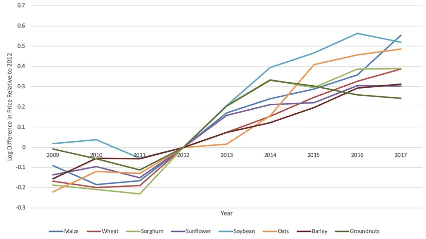
Next, we focus on whether the costs of the minimum wage hike were passed on to downstream firms
and final consumers through increased prices. First, we look at the external data on yearly crop prices
provided by the Department of Agriculture—specifically maize, wheat, sorghum, sunflower, soybean,
oats, barley, and groundnuts.4 In Figure 1b we plot the log difference in prices by crop in each year
and prices in 2012 (the year before the minimum wage hike). We find that the trend in prices before
the minimum wage hike was approximately flat, but following the minimum wage hike prices increased
sharply between 20 and 50 per cent. For example, the price of barley increased by approximately
30 per cent and the price of wheat increased by approximately 40 per cent. We also see this in firm
revenues, which reflect prices. We estimate Equation 1, replacing exposureit with an indicator for the
agricultural sector and with log sales as the outcome variable, Yit . Figure A1 presents the results. Again,
we find no evidence of pre-trends, or significant effects of the minimum wage on the agricultural sector
prior to the year of the minimum wage hike. We find that after the minimum wage increase there was
an approximately 30 per cent increase in agricultural revenue relative to other industries, significant
at the 95 per cent confidence level. Together, this suggests that much of the increase in costs from
the minimum wage hike was passed along to downstream buyers. We report consistent difference-in-
difference estimates of Equations 2 and 3 with log sales as the outcome variable and replacing exposureit
with an indicator for the agricultural sector, at both the industry and firm levels, in panel B of Table 1.
Both point estimates are positive and significant at the 95 per cent confidence level.
4 We present the raw price data in Table A4.
5Figure 1: Impact of minimum wage on agriculture industry
(a) Labour costs
(b) Crop prices
Note: panel A presents the event study estimates of Equation 1, replacing exposureit with an indicator for the agricultural
sector and log labour costs as the outcome variable, Yit . We plot the coefficients, βr , for each year, r, from the minimum wage
hike year. Industry and year fixed effects are included. Standard errors are robust. We include years from 2011 to 2017. Panel
B plots the log difference in price relative to 2012 for eight crops between 2009 to 2017.
Source: author’s construction based on data from National Treasury and UNU-WIDER (2019) and the Department of
Agriculture.
6Table 1: Impact of minimum wage on agriculture industry
Industry level Firm level
(1) (2) (3) (4) (5) (6)
Panel A: log labour costs
Agriculture × post 0.157∗∗∗ 0.087∗ 0.252∗∗∗ 1.116∗∗∗ 1.246∗∗∗ 0.400∗∗
(0.051) (0.051) (0.073) (0.204) (0.219) (0.175)
Average of control group 22.253 20.871 21.828 12.004 11.815 13.038
Number of observations 343 343 343 248954 210848 38106
Adjusted R-squared 0.976 0.983 0.961 0.593 0.574 0.661
Panel B: log sales
Agriculture × post 0.309∗∗∗ 0.195∗∗∗ 0.443∗∗∗ 0.120∗∗∗ 0.097∗∗∗ 0.130∗∗∗
(0.086) (0.054) (0.128) (0.029) (0.032) (0.036)
Average of control group 24.269 22.860 23.881 13.587 13.385 14.725
Number of observations 343 343 343 257,271 218,384 38,887
Adjusted R-squared 0.962 0.969 0.951 0.989 0.966 0.986
Industry/firm FE Yes Yes Yes Yes Yes Yes
Year FE Yes Yes Yes Yes Yes Yes
Sample All Small Large All Small Large
Note: this table presents estimates of Equation 2 in columns 1–3 and Equation 3 in columns 4–6, replacing exposureit with an
indicator for the agricultural sector. The outcome variable, Yit , is log labour costs in panel A, and log sales in panel B. Industry
and year fixed effects are included. In columns 1 and 4, the sample is all formal firms that are registered and active in 2011. In
columns 2 and 5, the sample is all formal firms that are registered, active, and classified as small in 2011. In columns 3 and 6,
the sample is all formal firms that are registered, active, and classified as medium to large in 2011. We include years from
2011 to 2017. Standard errors are clustered at the industry–year level in parentheses. * p < 0.10, ** p < 0.05, *** p < 0.01.
Source: author’s calculations based on data from National Treasury and UNU-WIDER (2019).
5.2 Impact on upstream exposed sectors
In this section, we present our main results on the impact of the minimum wage hike on industries
downstream from the agriculture sector. We find that there are large negative effects on employment,
sales, and assets from the minimum wage in industries with greater upstream exposure to the agriculture
sector, which fall largely on medium to large firms. We also find a reduction in profits for medium to
large firms.
First, we focus on the impact of the minimum wage on employment in industries downstream from the
agricultural sector. We estimate Equation 1 with log employment as the outcome variable, Yit . Figure
2a presents the results. We find no evidence of pre-trends, or significant effects of the minimum wage
on the sectors downstream from the agricultural sector prior to the year of the minimum wage hike. We
estimate that the causal effect of upstream exposure to the agricultural sector on employment is negative
and significant at the 95 per cent confidence level in all years following the minimum wage hike. We
find that increasing upstream exposure to the agriculture sector by one standard deviation results in a 2
per cent decrease in industry employment in all post-minimum wage hike years. We report consistent
difference-in-difference estimates of Equations 2 and 3 with log employment as the outcome variable,
at both the industry and firm levels, in columns 1 and 4 of panel A in Table 2, respectively. Both point
estimates are positive and significant at the 95 per cent confidence level. We also estimate the effects
for small and medium to large firms separately. We find that the effects are even larger for medium to
large firms, while they are still negative but insignificant for small firms. We present the difference-in-
difference results for medium to large firms in columns 3 and 6 of panel A in Table 2. We estimate
Equation 1 with log employment as the outcome variable, Yit , restricting the sample to medium to large
firms, and present the results in Figure 2a. We find that increasing upstream exposure to the agriculture
sector by one standard deviation results in a 5 per cent decrease in industry employment for medium
to large firms post-minimum wage hike, significant at the 95 per cent confidence level. We present the
difference-in-difference results for small firms in columns 2 and 5 of panel A in Table 2. We find that
7the effects of the minimum wage on small firms in upstream-exposed industries are insignificant, though
negative in sign.
Figure 2: Impact of upstream exposure to the minimum wage (agricultural) sector: overall
(a) Employment (b) Sales
(c) Assets (d) Profits
Note: this figure presents the event study estimates of Equation 1. The outcome variable, Yit , is (a) log employment, (b) log
sales, (c) log assets, and (d) log profits. We plot the coefficients, βr , for each year, r, from the minimum wage hike year.
Industry and year fixed effects are included. The sample is all formal firms that are registered and active in 2011. Standard
errors are robust. We include years from 2011 to 2017.
Source: author’s construction based on data from National Treasury and UNU-WIDER (2019).
Second, we look at the impact of the minimum wage on sales in industries downstream from the agri-
cultural sector. We find that the effects are significant only for medium to large firms, but insignificant
for small firms. Again, we find no evidence of pre-trends. We estimate Equation 1 with log sales as the
outcome variable, Yit , restricting the sample to medium to large firms, and present the results in Figure
3b. We estimate that the causal effect of upstream exposure to the agricultural sector on sales is nega-
tive, with the negative effect growing slightly over time, significant at the 95 per cent confidence level
one year after the minimum wage hike. We find that increasing upstream exposure to the agriculture
sector by one standard deviation results in a 2 per cent decrease in industry sales in 2013, which then
grows into a larger 5 per cent decrease by 2016 and 2017. The results are similar when we consider both
small and medium to large firms together, as in Figure 2b, with negative and growing effects over time,
except with smaller coefficients and with estimates only significant at the 95 per cent confidence level
two years after the minimum wage hike. We estimate Equations 2 and 3 with log sales as the outcome
variable and present the difference-in-difference results for all firms, small firms, and medium to large
firms separately, at both the industry and firm level, in panel B of Table 2. We find that the estimates for
medium to large firms are negative and significant at the 95 per cent confidence level at both the firm
and industry level, while the estimates for small firms are insignificant.
8Table 2: Impact of upstream exposure
Industry level Firm level
(1) (2) (3) (4) (5) (6)
Panel A: log employment
Upstream exposure × post –1.853∗∗∗ –0.317 –5.040∗∗∗ –0.374∗∗ 0.010 –0.679∗∗∗
(0.519) (0.273) (1.307) (0.182) (0.171) (0.244)
Average of control group 10.078 8.952 9.519 2.407 2.239 3.368
Number of observations 336 336 336 192,715 164,509 28,206
Adjusted R-squared 0.954 0.977 0.939 0.983 0.954 0.984
Panel B: log sales
Upstream exposure × post –1.164∗ –0.179 –3.573∗∗∗ 0.133 0.169 –0.178∗∗
(0.596) (0.427) (1.281) (0.114) (0.122) (0.088)
Average of control group 24.236 22.826 23.852 16.618 16.475 17.728
Number of observations 336 336 336 124,960 111,152 13,808
Adjusted R-squared 0.962 0.968 0.956 0.962 0.967 0.895
Panel C: log profits/standardized profit
Upstream exposure × post –0.427 –0.063 –2.548∗∗ –0.198∗∗ –3.489∗ –0.042∗∗∗
(0.387) (0.197) (1.065) (0.096) (1.868) (0.011)
Average of control group 23.277 21.790 22.886 –0.027 0.114 –0.073
Number of observations 336 336 336 124,960 111,152 13,808
Adjusted R-squared 0.972 0.978 0.961 0.846 0.846 0.870
Panel D: log assets
Upstream exposure × post –4.386∗∗∗ –0.212 –6.411∗∗∗ –0.363 –0.076 –0.437∗
(1.359) (1.402) (2.035) (0.545) (0.676) (0.235)
Average of control group 23.981 21.997 23.781 15.968 15.757 17.516
Number of observations 336 336 336 102,864 90,934 11,930
Adjusted R-squared 0.925 0.952 0.900 0.908 0.916 0.869
Panel E: log firm count/firm exist
Upstream exposure × post 0.159 0.251 –0.577 –0.039 –0.033 –0.105
(0.158) (0.155) (0.396) (0.064) (0.062) (0.115)
Average of control group 5.675 5.436 3.973 0.843 0.845 0.835
Number of observations 336 336 336 258,651 221,255 37,396
Adjusted R-squared 0.996 0.995 0.989 0.470 0.468 0.485
Industry/firm FE Yes Yes Yes Yes Yes Yes
Year FE Yes Yes Yes Yes Yes Yes
Sample All Small Large All Small Large
Note: this table presents estimates of Equation 2 in columns 1–3 and Equation 3 in columns 4–6. The outcome variable, Yit , is
log employment in panel A; log sales in panel B; log profits in columns 1–3 and profit normalized with mean 0 and standard
deviation 1 in columns 4–6 in panel C; log assets in panel D; and log firm count in columns 1–3 and an indicator that equals 1 if
the firm exists and 0 otherwise in columns 4–6 in panel E. Industry and year fixed effects are included in columns 1–3. Firm
and year fixed effects are included in columns 4–6. In columns 1 and 4, the sample is all formal firms that are registered and
active in 2011. In columns 2 and 5, the sample is all formal firms that are registered, active, and classified as small in 2011. In
columns 3 and 6, the sample is all formal firms that are registered, active, and classified as medium to large in 2011. We
include years from 2011 to 2017. Standard errors are clustered at the industry–year level in parentheses. * p < 0.10,
** p < 0.05, *** p < 0.01.
Source: author’s calculations based on data from National Treasury and UNU-WIDER (2019).
Next, we look at the impact of the minimum wage on assets in industries downstream from the agricul-
tural sector. Again, we find that the effects are significant only for medium to large firms, and insignifi-
cant for small firms. We estimate Equation 1 with log assets as the outcome variable, Yit , restricting the
sample to medium to large firms, and present the results in Figure 3c. Again, we find no evidence of
pre-trends. We find that the causal effect of upstream exposure to the agricultural sector on assets effects
only appear starting in 2014, the year after the minimum wage hike, in contrast to other outcome vari-
ables where there is an immediate effect the year of the policy change. We find that increasing upstream
exposure to the agriculture sector by one standard deviation results in an approximately 6 per cent de-
9crease in industry assets post-minimum wage hike. The results are similar when we consider both small
and medium to large firms together, as in Figure 2c, with significant negative effects appearing starting
in 2014, except with slightly smaller coefficients. We estimate Equations 2 and 3 with log assets as the
outcome variable and present the difference-in-difference results for all firms, small firms, and medium
to large firms separately, at both the industry and firm level, in panel C of Table 2. We find that the
estimates for medium to large firms are negative and significant at the 95 per cent confidence level at
both the firm and industry level, while the estimates for small firms are insignificant.
Figure 3: Impact of upstream exposure to the minimum wage (agricultural) sector: medium to large firms
(a) Employment (b) Sales
(c) Assets (d) Profits
Note: this figure presents the event study estimates of Equation 1. The outcome variable, Yit , is (a) log employment, (b) log
sales, (c) log assets, and (d) log profits. We plot the coefficients, βr , for each year, r, from the minimum wage hike year.
Industry and year fixed effects are included. The sample is all formal firms that are registered, active, and classified as medium
to large firms in 2011. Standard errors are robust. We include years from 2011 to 2017.
Source: author’s construction based on data from National Treasury and UNU-WIDER (2019).
From the results so far, we can conclude that medium to large firms in industries with greater upstream
exposure to the agricultural sector experienced greater contraction after the minimum wage hike. Small
firms are more likely to source from informal producers of agriculture who do not adhere to the minimum
wage. Data from a survey of 48,000 firms shows that size is strongly positively correlated with share
of suppliers that are formal (or registered) (De Paula and Scheinkman 2011). Thus, the costs of the
minimum wage hike are less likely to be passed downstream to small firms, while medium to large firms
that source from the formal sector will be affected. Our results indicate that accounting for informality
is critical in quantifying network spillovers from labour policies.
Now we turn to looking at whether there were also negative effects on profits. Again, we find that the
effects are significant only for medium to large firms, but insignificant at the 95 per cent confidence
level for small firms. We estimate Equation 1 with log profits as the outcome variable, Yit , restricting
the sample to medium to large firms, and present the results in Figure 3d. Again, we find no evidence
of pre-trends. We estimate that the causal effect of upstream exposure to the agricultural sector on
profits is negative, with the negative effect growing slightly over time, significant at the 95 per cent
confidence level two years after the minimum wage hike. We find that increasing upstream exposure to
10the agriculture sector by one standard deviation results in a decrease in industry sales by less than 1 per
cent in 2013, increasing to a decrease in industry sales of approximately 4 per cent in 2016 and 2017.
The results are similar when we consider both small and medium to large firms together, as in Figure 2b,
with negative and growing effects over time, except with smaller coefficients and with estimates only
significant at the 95 per cent confidence level three years after the minimum wage hike. We estimate
Equation 2 with log profits as the outcome variable, and Equation 3 with profits normalized, such that
the mean is 0 and the standard deviation is 1, as the outcome variable.5 We present the difference-in-
difference results for all firms, small firms, and medium to large firms separately, at both the industry
and firm levels, in panel D of Table 2. We find that the estimates for medium to large firms are negative
and significant at the 95 per cent confidence level at both the firm and industry levels, while the estimates
for small firms are insignificant.
Last, we investigate whether the results are driven by firm exit. We do not find any evidence of firm
exit across all our specifications. We estimate Equations 2 and 3 with log firm count and a dummy
for the firm being active as the outcome variable for the industry- and firm-level analysis respectively,
and present the difference-in-difference results for all firms, small firms, and medium to large firms
separately in panel E of Table 2. We find that all estimates are null and insignificant at the 95 per cent
confidence level. Thus, we conclude that our results are driven by downsizing at the firm level rather
than firm exit.
5.3 Robustness
First, we test the validity of our empirical strategy with a placebo test. Instead of estimating the effect
of upstream exposure to the agricultural sector, we estimate upstream exposure to the financial sector.
The financial sector is the industry least indirectly exposed to the agriculture sector via supply chains.
Thus, there should be no relationship between upstream exposure to the financial sector and outcomes
post-minimum wage hike. We estimate Equations 2 and 3 for each of our outcome variables, replacing
exposureit with upstream exposure to the financial sector instead of the agricultural sector. We present
the results in columns 1–3 of Table A5. We find that all the estimates are null and insignificant at the
95 per cent confidence level across both small and medium to large firms. We repeat the exercise for a
number of industries, finding similar results. We present the results for the nuclear fuel industry and for
the electricity, gas, and water industry in columns 4–9 of Table A5.
Next, we find that our main results are similar when we relax our balanced sample restriction. Instead
of restricting our sample to firms that existed prior to the minimum wage hike in 2011, we include all
firms in the sample. We now classify firms as small or medium to large according to the first year that
they are active in our sample period, instead of their category in 2011. We present our results in Table
A6 and Figure A2. We find that our results are quantitatively similar.
We also show that our results are robust to an alternate measure of upstream exposure. Instead of
using direct inputs to capture upstream exposure, here we account for indirectly required inputs to a
sector (suppliers of the industry’s immediate supplier). We redefine upstream exposure as the value of
both indirect and direct inputs from the agriculture sector divided by the industry’s total output value.
Columns 1–3 in Table A7 show that accounting for indirectly required inputs yields similar results as in
our main specification.
We also find that our results are robust to weighting each industry by its respective size in 2011. We
present the results in columns 4–6 in Table A7 and find similar results as in our main specification.
5 Since firm profits can be negative.
11Last, we investigate whether there may be regional heterogeneity in the results. We split South Africa
into its north and south regions.6 The south region’s economy is centred around Cape Town and Port
Elizabeth, while in the north region the major clusters are Johannesburg/Pretoria, and KwaZulu-Natal.
We estimate Equation 2 including an additional interaction for the outcome share of firms located in the
north region. Table A8 presents the results. We find that the contractionary effects of upstream exposure
to the minimum wage sector is larger for firms in the south region. This is consistent with Statistics
South Africa data that indicates that the south region is more agriculture-intensive.
6 Conclusion
This paper provides new evidence that the minimum wage has significant spillover effects on firms ex-
posed to the minimum wage indirectly via firm supply chains. We study the impact of a 50 per cent agri-
cultural minimum wage hike in South Africa on the outcomes of firms upstream from the agriculture sec-
tor. We find that industries with greater upstream exposure to the agriculture sector experienced greater
decreases in assets, sales, and employment for medium to large firms following the minimum wage
increase. Small firms source from informal agriculture producers who do not adhere to the minimum
wage. The results suggest that accounting for informality is critical in quantifying network spillovers
from labour policies. These results suggest that the minimum wage has negative second-order effects
through firm supply chain networks, which must be considered by policy-makers and other researchers
studying the impact of the minimum wage.
References
Aaronson, D., E. French, and I. Sorkin (2013). ‘Firm Dynamics and the Minimum Wage: A Putty-Clay Approach’.
Working Paper 2013-23. Chicago, IL: Federal Reserve Bank of Chicago. https://doi.org/10.2139/ssrn.2369447
Aaronson, D., E. French, I. Sorkin, and T. To (2018). ‘Industry Dynamics and the Minimum Wage: A Putty-Clay
Approach’. International Economic Review, 59(1): 51–84. https://doi.org/10.1111/iere.12262
Barrot, J.-N., and J. Sauvagnat (2016). ‘Input Specificity and the Propagation of Idiosyncratic Shocks in Produc-
tion Networks’. Quarterly Journal of Economics, 131(3): 1543–92. https://doi.org/10.1093/qje/qjw018
Bhorat, H., R. Kanbur, and B. Stanwix (2014). ‘Estimating the Impact of Minimum Wages on Employment,
Wages, and Non-Wage Benefits: The Case of Agriculture in South Africa’. American Journal of Agricultural
Economics, 96(5): 1402–19. https://doi.org/10.1093/ajae/aau049
Boehm, C.E., A. Flaaen, and N. Pandalai-Nayar (2019). ‘Input Linkages and the Transmission of Shocks: Firm-
Level Evidence from the 2011 Tōhoku Earthquake’. Review of Economics and Statistics, 101(1): 60–75. https:
//doi.org/10.1162/rest_a_00750
Card, D., and A.B. Krueger (1995). ‘Time-Series Minimum-Wage Studies: A Meta-analysis’. American Economic
Review, 85(2): 238–43.
Conradie, B. (2005). ‘Wages and Wage Elasticities for Wine and Table Grapes in South Africa’. Agrekon, 44(1):
138–56. https://doi.org/10.1080/03031853.2005.9523706
De Paula, A., and J.A. Scheinkman (2011). ‘The Informal Sector: An Equilibrium Model and Some Empirical
Evidence from Brazil’. Review of Income and Wealth, 57: S8–S26. https://doi.org/10.1111/j.1475-4991.2011.
00450.x
6South region: Western Cape, Eastern Cape, Northern Cape, Free State, KwaZulu-Natal. North region: Gauteng, North West,
Mpumalanga, Limpopo.
12Department of Agriculture (2020). ‘Economic Review of the South African Agriculture 2019/20’. Technical Re-
port. Pretoria: Department of Agriculture, Land Reform & Rural Development.
Di Giovanni, J., A.A. Levchenko, and I. Mejean (2014). ‘Firms, Destinations, and Aggregate Fluctuations’. Econo-
metrica, 82(4): 1303–40. https://doi.org/10.3982/ECTA11041
Dinkelman, T., and V. Ranchhod (2010). ‘Evidence on the Impact of Minimum Wage Laws in an Informal Sector:
Domestic Workers in South Africa’. SALDRU Working Paper 44. Cape Town: SALDRU.
Dix-Carneiro, R., and B.K. Kovak (2019). ‘Margins of Labor Market Adjustment to Trade’. Journal of Interna-
tional Economics, 117: 125–42. https://doi.org/10.1016/j.jinteco.2019.01.005
Dix-Carneiro, R., P.K. Goldberg, C. Meghir, and G. Ulyssea (2021). ‘Trade and Informality in the Presence of La-
bor Market Frictions and Regulations’. Working Paper 28391. Cambridge, MA: National Bureau of Economic
Research. https://doi.org/10.3386/w28391
Doucouliagos, H., and T.D. Stanley (2009). ‘Publication Selection Bias in Minimum-Wage Research? A
Meta-Regression Analysis’. British Journal of Industrial Relations, 47(2): 406–28. https://doi.org/10.1111/j.
1467-8543.2009.00723.x
Dube, A., T.W. Lester, and M. Reich (2010). Minimum Wage Effects Across State Borders: Estimates Using
Contiguous Counties. Review of Economics and Statistics, 92(4): 945–64. https://doi.org/10.1162/REST_a_
00039
Foerster, A.T., P.-D.G. Sarte, and M.W. Watson (2011). ‘Sectoral Versus Aggregate Shocks: A Structural Factor
Analysis of Industrial Production’. Journal of Political Economy, 119(1): 1–38. https://doi.org/10.1086/659311
Garbers, C., R. Burger, and N. Rankin (2015). ‘The Impact of the Agricultural Minimum Wage on Farmworker
Employment in South Africa: A Fixed Effects Approach’. Unpublished Masters Thesis. Cape Town: Stellen-
bosch University.
Goldberg, P.K., and N. Pavcnik (2016). ‘The Effects of Trade Policy’. In K. Bagwell and R.W. Staiger (eds),
Handbook of Commercial Policy, volume 1. Amsterdam: Elsevier.
Hall, P. (2014). Cities of Tomorrow: An Intellectual History of Urban Planning and Design Since 1880. Chichester:
Wiley.
Harasztosi, P., and A. Lindner (2019). ‘Who Pays for the Minimum Wage?’. American Economic Review, 109(8):
2693–727. https://doi.org/10.1257/aer.20171445
Lehohla, P. (2017). Input-Output Table for South Africa, 2012. Technical Report 04-04-02. Pretoria: Statistics
South Africa.
MaCurdy, T. (2015). ‘How Effective Is the Minimum Wage at Supporting the Poor?’. Journal of Political Econ-
omy, 123(2): 497–545. https://doi.org/10.1086/679626
McCaig, B., and N. Pavcnik (2018). ‘Export Markets and Labor Allocation in a Low-Income Country’. American
Economic Review, 108(7): 1899–941. https://doi.org/10.1257/aer.20141096
Murray, J., and C. Van Walbeek (2007). ‘Impact of the Sectoral Determination for Farm Workers on the South
African Sugar Industry: Case Study of the KwaZulu-Natal North and South Coasts’. Agrekon, 46(1): 94–112.
https://doi.org/10.1080/03031853.2007.9523763
National Treasury and UNU-WIDER (2019). ’CIT-IRP5 Firm Panel 2008-2017 [dataset]. Version 3.4’. Pretoria:
South African Revenue Service [producer of the original data], 2018. Pretoria: National Treasury and UNU-
WIDER [producer and distributor of the harmonized dataset], 2019.
Neumark, D., and W.L. Wascher (2010). Minimum Wages. Cambridge, MA: MIT Press.
Pieterse, D., E. Gavin, and C.F. Kreuser (2018). ‘Introduction to the South African Revenue Service and National
Treasury Firm-Level Panel’. South African Journal of Economics, 86(S1): 6–39. https://doi.org/10.1111/saje.
12156
13Ponczek, V., and G. Ulyssea (2020). ‘Is Informality an Employment Buffer? Evidence from the Trade Liberaliza-
tion in Brazil’. Unpublished Manuscript.
Ranchhod, V., and I. Bassier (2017). ‘Estimating the Wage and Employment Effects of a Large Increase in South
Africa’s Agricultural Minimum Wage’. REDI3x3 Working Paper 38. Cape Town: SALDRU.
Stigler, G.J. (1946). ‘The Economics of Minimum Wage Legislation’. American Economic Review, 36(3): 358–65.
14Appendix A: Extra figures and tables
Table A1: Summary statistics: firm level
Count Mean Std dev. Min. Max. Q1 Median Q3
Employment (thousands) 170,579 0.087 0.976 0.000 97.765 0.001 0.010 0.035
Sales (billion rand) 170,579 0.135 1.674 0.000 177.136 0.000 0.007 0.035
Assets (billion rand) 170,579 0.298 11.960 0.000 1305.112 0.000 0.004 0.020
Gross profits (billion rand) 170,579 0.047 0.837 –1.811 94.376 0.000 0.003 0.012
Firms exist 170,579 0.764 0.425 0.000 1.000 1.000 1.000 1.000
Upstream exposure 170,579 0.008 0.038 0.000 0.498 0.000 0.000 0.001
Note: this table presents summary statistics at the firm level. The sample is all firms that are registered and active in 2011. We
include years 2011–17.
Source: author’s calculations based on data from National Treasury and UNU-WIDER (2019).
Table A2: Summary statistics: industry level
Count Mean Std dev. Min. Max. Q1 Median Q3
Employment (thousands) 336 53.425 81.781 0.127 490.394 9.780 22.269 66.471
Sales (billion rand) 336 93.691 177.152 0.061 1329.739 9.157 39.706 104.380
Assets (billion rand) 336 206.580 726.830 0.014 6505.233 5.735 29.234 110.581
Gross profits (billion rand) 336 32.759 43.701 0.047 260.622 3.400 15.040 45.406
Number of firms 336 677.152 1210.560 11.000 7521.000 114.000 251.000 565.000
Upstream exposure 336 0.025 0.082 0.000 0.498 0.000 0.001 0.002
Note: this table presents summary statistics at the industry level. The sample is all firms that are registered and active in 2011.
We include years 2011–17.
Source: author’s calculations based on data from National Treasury and UNU-WIDER (2019).
Table A3: Summary statistics for agriculture industry: firm level
Count Mean Std dev. Min. Max. Q1 Median Q3
Employment (thousands) 9,759 0.118 0.428 0.000 20.043 0.002 0.024 0.089
Sales (billion rand) 9,759 0.078 0.451 0.000 13.474 0.000 0.015 0.041
Assets (billion rand) 9,759 0.087 0.430 0.000 14.541 0.007 0.023 0.057
Gross profits (billion rand) 9,759 0.030 0.155 –0.171 6.637 0.000 0.009 0.023
Firms exist 9,759 0.770 0.421 0.000 1.000 1.000 1.000 1.000
Labour wages (billion rand) 9,759 0.007 0.041 0.000 1.497 0.000 0.001 0.004
Labour costs (billion rand) 9,759 0.008 0.046 0.000 1.658 0.000 0.002 0.005
Note: this table presents summary statistics at the firm level for the agriculture industry. The sample is all agriculture sector
firms that are registered and active in 2011. We include years 2011–17.
Source: author’s calculations based on data from National Treasury and UNU-WIDER (2019).
15Table A4: Agriculture prices by year (R/c per ton)
Year Maize Wheat Sorghum Sunflower Soybean Oats Barley Groundnuts
2009 1,606.66 2,307.46 1,774.43 4,271.88 4,026.26 2,055.41 2,300.31 6,122.10
2010 1,440.96 1,607.67 1,494.65 2,854.58 3,187.39 1,297.47 2,125.90 6,360.69
2011 1,097.91 2,303.68 1,383.50 2,953.46 2,527.96 2,170.08 2,006.34 4,659.65
2012 1,691.66 2,369.08 1,671.61 3,735.57 3,176.39 2,003.71 2,277.23 5,200.52
2013 2,200.12 2,914.55 2,675.01 4,396.90 3,684.46 2,051.58 2,498.99 8,287.26
2014 2,026.56 2,880.31 2,691.62 4,844.00 4,691.65 2,270.50 2,519.07 8,755.87
2015 2,122.15 3,052.85 2,626.78 4,435.47 5,549.81 2,945.49 2,644.29 8,233.51
2016 2,502.41 3,772.44 2,380.90 4,552.42 4,731.87 4,153.08 3,098.03 7,581.89
2017 2,518.58 3,704.64 3,434.39 6,064.02 6,197.36 2,738.69 3,352.15 7,721.68
Note: this table presents raw price data by crop between 2009 and 2017.
Source: author’s calculations based on data from the Department of Agriculture.
Table A5: Placebo tests
Financial intermediation Nuclear fuel Electricity, gas, and water
(1) (2) (3) (4) (5) (6) (7) (8) (9)
Panel A: log employment
Upstream exposure × post –0.162 –0.025 –0.697 –0.608 –0.455 –0.493 –0.259 –1.863 0.139
(0.664) (0.302) (0.746) (0.398) (0.439) (0.476) (2.207) (0.982) (4.151)
Average of control group 10.118 9.001 9.556 10.118 9.001 9.558 10.118 9.001 9.558
Number of observations 336 336 336 336 336 336 336 336 336
Adjusted R-squared 0.953 0.982 0.926 0.954 0.979 0.928 0.954 0.979 0.927
Panel B: log sales
Upstream exposure × post 0.496 –0.988 0.603 –0.852 0.317 –1.049 –0.409 –0.629 2.793
(0.585) (0.741) (0.517) (0.709) (0.354) (0.901) (2.242) (1.027) (2.847)
Average of control group 24.264 22.860 23.881 24.264 22.860 23.881 24.264 22.860 23.881
Number of observations 336 336 336 336 336 336 336 336 336
Adjusted R-squared 0.966 0.970 0.954 0.963 0.969 0.951 0.962 0.970 0.950
Panel C: log profits
Upstream exposure × post 0.225 0.073 –0.023 –0.762 –0.010 –0.911 –0.822 1.103 0.977
(0.397) (0.245) (0.443) (0.584) (0.325) (0.766) (2.095) (0.979) (2.758)
Average of control group 23.305 21.830 22.911 23.305 21.830 22.911 23.305 21.830 22.911
Number of observations 336 336 336 336 336 336 336 336 336
Adjusted R-squared 0.975 0.980 0.961 0.972 0.979 0.959 0.971 0.979 0.958
Panel D: log assets
Upstream exposure × post 1.279 –0.303 1.424 –1.545 0.437 –1.442 –4.774 1.730 –0.464
(0.912) (0.629) (1.009) (1.500) (0.675) (1.600) (6.330) (3.623) (7.217)
Average of control group 24.009 22.040 23.805 24.009 22.040 23.805 24.009 22.040 23.805
Number of observations 336 336 336 336 336 336 336 336 336
Adjusted R-squared 0.913 0.956 0.879 0.921 0.953 0.891 0.921 0.954 0.890
Industry/firm FE Yes Yes Yes Yes Yes Yes Yes Yes Yes
Year FE Yes Yes Yes Yes Yes Yes Yes Yes Yes
Sample All Small Large All Small Large All Small Large
Note: this table presents estimates of Equation 2. We define upstream exposure as exposure to the financial intermediation
sector in columns 1–3, exposure to the nuclear fuel sector in columns 4–6, and exposure to the electricity, gas, and water
sector in columns 7–9. The outcome variable, Yit , is log employment in panel A, log sales in panel B, log profits in columns 4–6
in panel C, and log assets in panel D. Industry and year fixed effects are included. In columns 1, 4, and 7, the sample is all
formal firms that are registered and active in 2011. In columns 2, 5, and 8, the sample is all formal firms that are registered,
active, and classified as small in 2011. In columns 3, 6, and 9, the sample is all formal firms that are registered, active, and
classified as medium to large in 2011. We include years from 2011 to 2017. Standard errors are clustered at the industry–year
level in parentheses. * p < 0.05, ** p < 0.01, *** p < 0.001.
Source: author’s calculations based on data from National Treasury and UNU-WIDER (2019).
16Table A6: Robustness: unbalanced sample with all firms
Industry level Firm level
(1) (2) (3) (4) (5) (6)
Panel A: log employment
Upstream exposure × post –0.720∗∗∗ –0.134 –1.642∗∗∗ –0.426∗ –0.218 –0.649∗∗∗
(0.228) (0.199) (0.458) (0.220) (0.224) (0.239)
Average of control group 10.463 9.221 9.995 1.002 0.935 1.523
Number of observations 336 336 336 1,174,726 1,042,002 132,724
Adjusted R-squared 0.968 0.976 0.949 0.973 0.935 0.976
Panel B: log sales
Upstream exposure × post –0.446 0.306 –1.524∗∗ 0.133 0.169 –0.178∗∗
(0.425) (0.311) (0.673) (0.114) (0.122) (0.088)
Average of control group 24.522 22.877 24.206 16.618 16.475 17.728
Number of observations 336 336 336 124,960 111,152 13,808
Adjusted R-squared 0.971 0.964 0.957 0.962 0.967 0.895
Panel C: log profits/standardized profit
Upstream exposure × post 0.240 0.269 –0.461 –0.446∗∗ –8.086∗ –0.082∗∗∗
(0.211) (0.237) (0.446) (0.217) (4.331) (0.021)
Average of control group 23.565 21.916 23.216 0.034 0.596 0.002
Number of observations 336 336 336 124,960 111,152 13,808
Adjusted R-squared 0.976 0.970 0.959 0.846 0.846 0.870
Panel D: log assets
Upstream exposure × post –3.415∗∗∗ –0.267 –4.681∗∗∗ –0.363 –0.076 –0.437∗
(1.040) (0.586) (1.419) (0.545) (0.676) (0.235)
Average of control group 24.279 21.893 24.132 15.968 15.757 17.516
Number of observations 336 336 336 102,864 90,934 11,930
Adjusted R-squared 0.940 0.959 0.929 0.908 0.916 0.869
Industry/firm FE Yes Yes Yes Yes Yes Yes
Year FE Yes Yes Yes Yes Yes Yes
Sample All Small Large All Small Large
Note: this table presents estimates of Equation 2 in columns 1–3 and Equation 3 in columns 4–6. The outcome variable, Yit , is
log employment in panel A; log sales in panel B; log profits in columns 1–3 and profit normalized with mean 0 and standard
deviation 1 in columns 4–6 in panel C; log assets in panel D; and log firm count in columns 1–3 and an indicator which equals
1 if the firm exists and 0 otherwise in columns 4–6 in panel E. Industry and year fixed effects are included in columns 1–3. Firm
and year fixed effects are included in columns 4–6. In columns 1 and 4, the sample is all formal firms that are registered and
active in any year. In columns 2 and 5, the sample is all formal firms that are registered and active in any year, and classified
as small in its first active year. In columns 3 and 6, the sample is all formal firms that are registered and active in any year, and
classified as medium to large in their first active year. We include years from 2011 to 2017. Standard errors are clustered at the
industry–year level in parentheses. * p < 0.10, ** p < 0.05, *** p < 0.01.
Source: author’s calculations based on data from National Treasury and UNU-WIDER (2019).
17You can also read