Using Multiple Hypotheses to Improve Depth-Maps for Multi-View Stereo
←
→
Page content transcription
If your browser does not render page correctly, please read the page content below
Using Multiple Hypotheses to Improve
               Depth-Maps for Multi-View Stereo

                        Neill D.F. Campbell1 , George Vogiatzis2 ,
                        Carlos Hernández2 , and Roberto Cipolla1
      1
              Department of Engineering, University of Cambridge, Cambridge, UK
          2
               Computer Vision Group, Toshiba Research Europe, Cambridge, UK

      Abstract. We propose an algorithm to improve the quality of depth-
      maps used for Multi-View Stereo (MVS). Many existing MVS techniques
      make use of a two stage approach which estimates depth-maps from
      neighbouring images and then merges them to extract a final surface.
      Often the depth-maps used for the merging stage will contain outliers
      due to errors in the matching process. Traditional systems exploit redun-
      dancy in the image sequence (the surface is seen in many views), in order
      to make the final surface estimate robust to these outliers. In the case of
      sparse data sets there is often insufficient redundancy and thus perfor-
      mance degrades as the number of images decreases. In order to improve
      performance in these circumstances it is necessary to remove the outliers
      from the depth-maps. We identify the two main sources of outliers in a
      top performing algorithm: (1) spurious matches due to repeated texture
      and (2) matching failure due to occlusion, distortion and lack of texture.
      We propose two contributions to tackle these failure modes. Firstly, we
      store multiple depth hypotheses and use a spatial consistency constraint
      to extract the true depth. Secondly, we allow the algorithm to return an
      unknown state when the a true depth estimate cannot be found. By com-
      bining these in a discrete label MRF optimisation we are able to obtain
      high accuracy depth-maps with low numbers of outliers. We evaluate our
      algorithm in a multi-view stereo framework and find it to confer state-
      of-the-art performance with the leading techniques, in particular on the
      standard evaluation sparse data sets.

1   Introduction
The topic of multi-view stereo (MVS) reconstruction has become a growing area
of interest in recent years with many differing techniques achieving a high degree
of accuracy [1]. These techniques focus on producing watertight 3D models from
a sequence of calibrated images of an object, where the intrinsic parameters and
pose of the camera are known. In addition to providing a taxonomy of methods,
[1] also provides a quantitative analysis of performance both in terms of accuracy
and completeness. The top performers may be loosely divided into two groups.
The first group make use of techniques such as correspondence estimation, local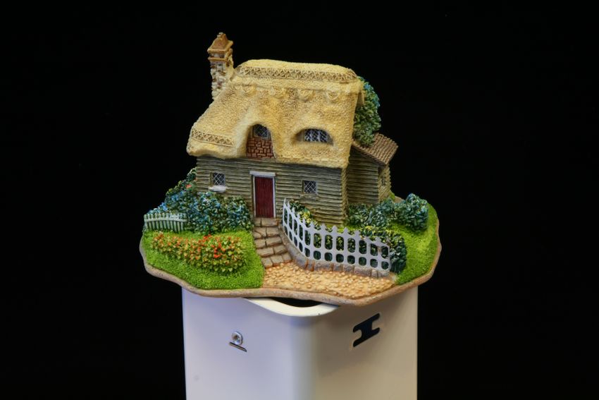
2       Neill D.F. Campbell et al.

Fig. 1: Depth map obtained from only three images of a model house. The
left image provides the recovered depth map which is rendered in the right image. As
well as achieving a high degree of accuracy on surface detail our algorithm has correctly
recovered the occlusion boundaries and removed outlying depth estimates

region growing and filtering to build up a final dense surface [13, 15, 16]. The
second group make use of some form of global optimisation strategy on a vol-
umetric representation to extract a surface [5, 14, 6, 12, 7]. A common strategy
is to split the reconstruction process into two stages. The first is to estimate a
series of depth-maps using local groups of the input images. The second stage
then attempts to combine these into a global surface estimate, making use of
registration and regularisation techniques. This two stage approach is an elegant
formulation which allows different techniques to be chosen independently for the
two stages. Some recent methods achieve a fast computation time by avoiding
a global optimisation when merging depth-maps [17, 18]. In this paper we focus
on the first of the two stages — local depth-map estimation.
    The estimation of local depth-maps is often performed using patch based
methods [2]. The work of [5] proposed the use of Normalised Cross-Correlation
(NCC) as the matching cost between two patches. This method offers good per-
formance for textured objects and has been the basis of [7, 6, 19]. In the first
stage of [5] a depth is estimated for each pixel independently. In the next stage
the algorithm looks for consensus in depth estimates from multiple depth-maps.
Since the individual depth-maps are known to contain outliers, this stage relies
upon redundancy in the depth-maps to reject the them. In data-sets containing
a large number of images (50-100) this approach performs quite well. In so called
sparse data-sets (10-20 images) one expects very little redundancy in the recon-
structed depth-maps, leading to a drop in reconstruction accuracy. This drop
is actually observed in the performance of [5] in sparse data-sets with ground
truth [1].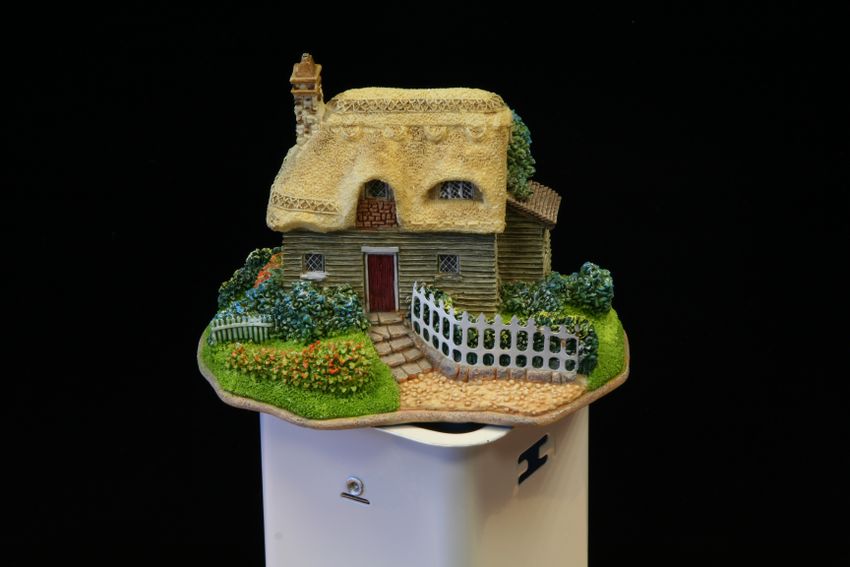
Using Multiple Hypotheses to Improve Depth-Maps for Multi-View Stereo        3

    In this paper we show that if individual depth-maps are filtered for outliers
prior to the fusion stage, good performance can be maintained in sparse data-
sets. Our strategy is to collect a list of good hypotheses for the depth of each
pixel. We then chose the optimal depth for each pixel by enforcing consistency
between neighbouring pixels in a depth-map. A crucial element of the filtering
stage is the introduction of a possible unknown depth hypothesis for each pixel,
which is selected by the algorithm when no consistent depth can be chosen. This
pre-processing of the depth-maps allows the global fusion stage to operate on
fewer outliers and consequently improve the performance under sparsity of data.
    The rest of the paper is laid out as follows: In § 2 we review relevant prior
work and discuss the differences of our approach. § 3 presents the use of NCC as
a photo-consistency metric for estimating depth-maps and provides an overview
of our algorithm to reduce outliers. § 4 provides the details of our depth-map
estimation algorithm, in particular the optimisation process. In § 5 we show
how to extend an existing MVS framework to include our depth-map estimation
procedure for the purpose of the experimental evaluation provided in § 6. Here
we display the improvements made to estimated depth-maps and also provided
a quantitative evaluation of the MVS results. The paper concludes with our
findings in § 7. This work was supported by a Schiff Scholarship and Toshiba
Research Europe.

2    Previous Work

A taxonomy of the established methods for dense stereo may be found in [2].
Most of these methods use matching costs to assign each pixel to a set of dis-
parity levels within the image. The earlier algorithms maintained relatively few
separate levels and were more targeted towards depth based segmentation rather
than detailed reconstruction. The latest algorithms [3] obtain depth-maps with
greater accuracy. Since these algorithms only have pairs of images available, they
can make no use of redundancy across multiple images in a data set and thus
they use spatial regularisation and optimisation schemes which attempt to in-
fer information about the depths. Whilst we also exploit a spatial regularisation
constraint, we only allow the optimisation to choose from a set of discrete depths,
well localised by the NCC peaks. This contrasts with methods which allow the
depth of each pixel to vary continuously whilst minimising some cost function.
    Some of the best performing algorithms make use of an occluded state. This
may be via an explicit estimation of a disparity map, for example [20] or inter-
nally as part of an optimisation routine [4]. We make use of the unknown state
in a similar manner however we also use it recognise the other failure modes of
NCC matching, discussed in § 3, since they are indistinguishable.
    The work of [5] proposed the robust NCC matching technique which we ex-
tend in our algorithm. Outlier rejection is accomplished through redundancy in
the image sequence. The works of [7, 6] have used derivatives of this technique
with slight modifications, for example the inclusion of a Parzen window to filter
the consensus matches in [6]. The work of [19] proposed a new, color normalised
4       Neill D.F. Campbell et al.

supersampling approach to correct for projective warping errors and also pro-
vided improved computation time with an efficient GPU implementation.
    Recent work has demonstrated that depth-map estimation and integration
paradigm may be used to produce accurate results with greatly reduced com-
putation time [18] or real-time [17]. Again the reliance upon redundancy in the
image sequence is paramount, for example the visibility computations of [17].
    Since our contribution affects only the depth-map estimation, the global stage
may be considered separately. The works of [23, 24] present complementary al-
gorithms for range image integration. Here, the depth-maps produced by our
algorithm would provide a suitable set of range images. The use of a volumetric
graph-cut to extract the surface was proposed in [14] and extended in [6] to in-
clude the robust NCC photoconsistency. Other works have shown the graph-cut
formulation to perform well as a global optimisation stage [12, 21].
    The work of [22] uses multiple depth hypotheses as a result of reflections
during the active 3D scanning of specular objects. Here a different framework,
also based on spatial consistency, is used to reject false matches. The work of [26]
makes use of multiple hypotheses for the related problem of new-view synthesis.
They also make use of an MRF optimisation, here using a truncated quadratic
kernel, to solve their synthesis problem.

3   Normalised Cross-Correlation for Photo-Consistency

Normalised Cross Correlation (NCC) may be used to define an error metric for
matching two windows in different images. Figure 2 provides an example of using
NCC and epipolar geometry to perform window based matching. If we fix a pixel
location in a reference image, for each possible depth away from that pixel we
get a corresponding pixel in the second image. By computing the NCC between
windows centred in those two pixels we can define a matching score as a function
of depth for the reference pixel. We refer to this function as the correlation curve
of the pixel. A typical correlation curve will exhibit a very sharp peak at the
correct depth, and possibly a number of secondary peaks in other depths.
    In [5] a depth-map is generated for each input image using this matching tech-
nique for neighbouring images. For each pixel a number of correlation curves are
computed (using a few of the neighbouring viewpoints) and the depth that gives
rise to most peaks in those curves is selected as the depth for that pixel. See [5]
or [6] for details. This process results in an independent depth estimate for each
pixel. These depth estimates will unavoidably contain a significant percentage
of outliers which must be dealt with in the subsequent step of [5] which is the
volumetric fusion of multiple depth-maps. In data sets with a large number of
images this is is overcome by the redundancy in the depth-estimates. The same
surface point is expected to be covered by many different depth-maps, some of
which will have the right depth estimate. In sparse data-sets however, each sur-
face point may be seen by as few as two or three depth-maps. It is therefore
crucial that outliers are minimised in the depth-map generation stage.
Using Multiple Hypotheses to Improve Depth-Maps for Multi-View Stereo                5

                      Select window in                Project into neighbouring image
                      reference image                        along epipolar line

                                    Locate matching window using
                                        maximum NCC score

                NCC Score

                                                      Depth

       Fig. 2: Normalised Cross-Correlation based window matching.

    In this work we focus on the two most significant failure modes of NCC
matching which are (1) the presence of repetitions in the texture and (2) com-
plete matching failure due to occlusion, distortion and lack of texture. These are
now described in more detail.

3.1   Repeating texture
In general, there is no guarantee that the appearance of a patch is unique across
the surface of the object. This results in correlation curve peaks at incorrect
depths due to repeated texture — ‘false’ matches (Fig. 2). A larger window
size is more likely to uniquely match to the true surface, reducing the number
of false matches. However the associated peak will be broader and less well
localised, reducing the accuracy of the depth estimate. The absolute value of the
NCC score at a peak reflects how well the two windows match. Thus one might
expect the peak with the maximum score to be the true peak. Unfortunately, the
appearance of false matches due to repeated texture may result in false peaks
having similar or even greater scores than the true surface peak (Fig. 3 (a)). To
identify the correct peak, we propose to apply a spatial consistency constraint
across neighbouring pixels in the depth-map. The underlying assumption is that
if a peak corresponds to the true surface, the neighbouring pixels should have
peaks at a similar depth. The exception to this is occlusion boundaries, which
are however catered for under the next failure mode.

3.2   Matching failure
The second failure mode is comprised of occlusion errors, distorted image win-
dows (due to slanted surfaces) and lack of texture. In all of these cases, the
correlation curve will not exhibit a peak at the true depth of the surface, re-
sulting in only false peaks. Furthermore no spatial consistency can be enforced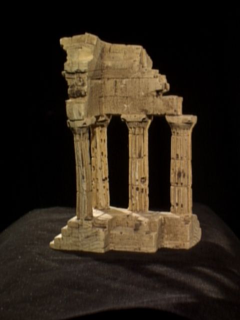
6      Neill D.F. Campbell et al.

between the pixel in question and its neighbours. In this situation we would like
to acknowledge that the depth at this pixel is unknown and should therefore
offer no vote for the surface location.
    In order to achieve these two goals we propose an optimisation strategy which
makes use of a discrete label Markov Random Field (MRF). The MRF allows
each pixel to choose a depth corresponding to one of the top NCC peaks which
is spatially consistent with neighbouring pixels or select an unknown label to
indicate that no such peak occurs and there is no correct depth estimate. This
process means that the returned depth map should only contain accurate depths,
estimated with a high degree of certainty, and an unknown label for pixels which
have no certain associated depth. Figure 3 illustrates the optimisation for a 1D
example of neighbouring pixels across an occlusion boundary.

                  NCC Peak          Maximum Peak           Chosen Peak

                                                                          NCC scores for neighbouring pixels
                                                   (a)              (a)

                                          (b)
                                Unknown

                                                   Depth

Fig. 3: Illustration of the MRF optimisation applied to neighbouring pix-
els. Existing method return the maximum peak which results in outliers in the depth
estimate. The MRF optimisation corrects an outlier to the true surface peak (a) and
introduces an unknown label at the occlusion boundary (b)

4   Depth Map Estimation

Our proposed algorithm estimates the depth for each pixel in the input images.
It proceeds in two stages: Initially we extract a set of possible depth values for
each pixel using NCC as a matching metric. We then solve a multi-label discrete
MRF model which yields the depth assignment for every pixel. One of the key
features in this process is the inclusion of an unknown state in the MRF model.
Using Multiple Hypotheses to Improve Depth-Maps for Multi-View Stereo             7

This state is selected when there is insufficient evidence for the correct depth to
be found.

4.1   Candidate Depths
The input to our algorithm is a set of calibrated images I and the output is
a set of corresponding depth-maps D. In the following, we describe how to ac-
quire a depth-map for a reference image Iref ∈ I. Let N (Iref ) denote a set of
‘neighbouring’ images to Iref .
     As proposed in § 3, we wish to obtain a hypothesis set of possible depths for
each pixel pi ∈ Iref . Taking each pixel in turn, we project the epipolar ray into a
second image In ∈ Iref and sample the NCC matching score over a depth range
ρi (z). We compute the score using a rectangular window centred at the projected
image co-ordinates. One of the advantages of the multiple depth hypotheses is
the ability to use a smaller matching window to provide a faster computation
and improved localisation of the surface. Once we have obtained the sampled
ray we store the top K peaks ρ̂i (zi,k ), k ∈ [1, K] with the greatest NCC score for
each pixel. Depending on the number of images available, and the width of the
camera baseline, this process may be repeated for other neighbouring images.
We then continue to the optimisation stage with a set of the best K possible
depths, and their corresponding NCC scores, over all neighbouring images of
Iref .

4.2   MRF Formulation
At this stage a set of candidate depths ρ̂i (zi,k ), k ∈ [1, K], for each pixel pi in
the reference image Iref has been assigned and we wish to determine the correct
depth map label for each pixel. As described in § 3, we also make use of an
unknown state to account for the failure modes of NCC matching.
    We model the problem as a discrete MRF where each each pixel has a set
of up to (K + 1) labels. The first K labels, fewer if an insufficient number of
peaks were found during the matching stage, correspond to the peaks in the
NCC function and have associated depths zi,k ∈ Zi and scores ρ̂i (zi,k ). The final
state is the unknown state U. If the optimisation returns this state, the pixel is
not assigned a depth in the final depth map. For each pixel we therefore form
                           0
an augmented label set zi,k   ∈ {Zi , U} to include the unknown state.
    The optimisation assigns a label k̄i ∈ {1 ... K, U)} to each pixel pi . The cost
function to be minimised consists of unary potentials for each pixel and pairwise
interactions over first order cliques. The cost of a labelling k̄ = {k̄i } is expressed
as                             X                X
                          E k̄ =       φ(k̄i ) +   ψ(k̄i , k̄j )                    (1)
                                    i          (i,j)

where i denotes a pixel and (i, j) denote neighbouring pixels.
   The following sections discuss the formulation of the unary potentials φ(·)
and pairwise interactions ψ(·, ·).
8 Neill D.F. Campbell et al.
4.3 Unary Potentials
The unary labelling cost is derived from the NCC score of the peak. We wish
to penalise peaks with a lower matching score since they are more likely to
correspond to an incorrect match due to occlusion or noise. The NCC process
will always return a score in the range [−1, 1]. As is common practice, [6], we
take an inverse exponential function to map this score to a positive cost.
The unary cost for the unknown state is set to a constant value φU . This term
serves two purposes. Firstly it acts as a cut-off threshold for peaks with poor NCC
scores which have no pairwise support (neighbouring peaks of similar depth).
This mostly accounts for peaks which are weakly matched due to distortion or
noise. Secondly it acts as a truncation on the depth disparity cost of the pairwise
term. By assigning a low pairwise cost between peaks and the unknown state,
the constant unary cost will effectively act as a threshold on the depth disparity
to handle the case of an occlusion boundary. Thus the final unary term is given
by
λ e−β ρ̂i (zi,x ) x ∈ [1 ... K]
φ ki = x = . (2)
φU x= U
4.4 Pairwise Interactions
The pairwise labelling cost is derived from the disparity in depths of neighbouring
peaks. As has been previously mentioned, this term is not intended to provide a
strong regularisation of the depth map. Instead it is used to try and determine
the correct peak, corresponding to the true surface location, out of the returned
peaks. We observe that the correct peak may not have the maximum score.
Therefore if there is strong agreement on depth between neighbouring peaks, we
take this to be the true location of the surface.
When dealing with the depth disparity term we are really considering surface
orientation; whether the surface normal is pointing towards or away from the
camera. Under a perspective projection camera model it is therefore necessary
to correct for the absolute depth of the peaks rather than simply taking the
difference in depth. We perform this correction by dividing by the average depth
of the two peaks. The resulting pairwise term is given by
zi,x − zj,y
2 x ∈ [1 ... K] y ∈ [1 ... K]
(zi,x + zj,y )
ψU x= U y ∈ [1 ... K] . (3)
ψ ki = x, kj = y =
ψU x ∈ [1 ... K] y = U
0 x= U y= U
We set ψU to a small value to encourage regions with many pixels labelled
as unknown to coalesce. This acts as a further stage of noise reduction since
it prevents spurious peaks with high scores but no surrounding support from
appearing in regions of occlusion.
Using Multiple Hypotheses to Improve Depth-Maps for Multi-View Stereo       9

4.5    Optimisation
To obtain the final depth map we need to determine the optimal labelling k̂ such
that
                                     X           X
                  E( k̂ ) = arg min    φ(k̄i ) +       ψ(k̄i , k̄j ) .       (4)
                                (k̄) i           (i,j)

Since in the general case this is an NP-hard problem we must use an approximate
minimisation algorithm to achieve a solution. The most well-known techniques
for solving problems of this nature are based on graph-cuts and belief propaga-
tion. Instead, we use the recently developed sequential tree-reweighted message
passing algorithm, termed TRW-S, of [8]. This has been shown to outperform
belief propagation and graph-cuts in tests on stereo matching using a discrete
number of disparity levels. In addition to minimising the energy, the algorithm
estimates a lower bound on the energy at each iteration which is useful in check-
ing for convergence and evaluating the performance of the algorithm. We should
note, however, that we are by no means guaranteed that the lower bound is
attainable.

5     Extension to Multi-View Stereo Framework
As previously discussed, the detailed evaluation of [1] demonstrates that volu-
metric methods display state-of-the-art performance both in terms of accuracy
and completeness. Some of the most successful create a 3D cost field within a
volume and the reconstruction task is then to extract the optimal surface from
this volume. Algorithms developed for segmentation problems are commonly
used to extract the surface.
    In order to evaluate the improvement to multi-view stereo we combined our
depth map estimation with a modified implementation of the volumetric regu-
larisation framework of [6]. This method uses a volumetric graph-cut to recover
the surface from an array of voxels. Each voxel becomes a node in a 3D binary
MRF where the voxel must be labelled as inside or outside the object. The MRF
formulation allows for two terms in the cost function. The first is the unary
foreground/background labelling cost. This encodes the likelihood that a par-
ticular voxel is part of the object or empty space. The recent work of [9] shows
how depth maps may be used to evaluate a probabilistic visibility measure for
each voxel in the volume. This term may be used to estimate whether or not
the voxel in question resides in empty space and is therefore visible from the
cameras. From this it is possible to derive an appropriate cost for the unary
term related to the likelihood of visibility. The second term is the pairwise dis-
continuity cost. This term represents the likelihood that the surface boundary
lies between two neighbouring voxels. This term may be derived directly from
the individual depth maps projected into the volume.
    In [25] the authors show that the energy cost is a discrete approximation to
the sum of a weighted surface area of the boundary (the pairwise terms) and
a weighted volume of the object (the unary terms). This framework is ideal for
10 Neill D.F. Campbell et al. use with our depth maps since it provides global regularisation using all the available data. This is a key advantage of our approach. Rather than perform regularisation on individual depth maps to recover uncertain regions, we only return depths with a high degree of confidence associated with them. Thus other depth maps may be able to fill in the areas where a particular depth map is uncertain. In the event that there are still regions of the surface which are not determined precisely by any of the depth maps, the regularisation should be performed by a global method which takes into account the data from all the depth maps rather than an amalgamation of estimates from individual depth maps. 5.1 Depth Map Acquisition The first stage of the reconstruction process is to acquire the depths maps. Our method is to select an image and project rays into the nearest neighbouring im- ages in a sequential process. We maintain a cumulative store of the K top scoring NCC peaks for each pixel. This provides an even greater degree of robustness against occlusion than the technique of [6] and is easier to implement in a parallel environment such as a GPU. Rather than requiring peaks from multiple images to fall in the same location, we only have to accurately observe a surface location in a single pair of images and rely on the surrounding support of peaks to identify the correct peaks. The speed of the depth map computation maybe increased by using the object silhouettes to avoid performing NCC matching calculations in regions outside the possible surface locations. Extraction of silhouettes for multi-view stereo may be performed as an automatic process [10]. 5.2 Surface Recovery Integrating our depth maps with the framework of [6] and [9] is a simple and elegant process. For the visibility volume we may project the same probability of visibility along each ray as [9] when we have a known depth. For pixels labelled as unknown we simply project a likelihood of 0.5 to indicate that this pixel provides no information about visibility. For the discontinuity cost we adopt a ‘binning’ approach. For each voxel in the discontinuity volume we take the sum of the projected depths of all the pixels in all the depth maps which fall inside the voxel, weighted by their NCC scores. If a pixel is labelled as unkown then it plays no part in the discontinuity cost. The final optimisation follows in the same manner as [6] with the graph-cut used to segment the volume. The iso-surface is extracted and smoothed using a snake [5] to perform ‘intelligent’ smoothing making use of the photoconsistency volume. 6 Experiments 6.1 Implementation To improve the computation time for our depth maps we perform the NCC matching by taking advantage of the parallel processing and texture facilities of
Using Multiple Hypotheses to Improve Depth-Maps for Multi-View Stereo        11

the GPU of modern graphics cards. The GPU code improves performance by up
to an order of magnitude depending on the window size. On of the advantages of
our method is the ability to use small windows which result in greater precision of
the surface location but which introduce a significant amount of noise which will
adversely affect many of the existing techniques. The use of the smaller window
also results in a greater saving in computational efficiency since the GPU offers
improved performance with small kernels.
    For the optimisation of the discrete MRF for the depth map we use the TRW-
S implementation of Kolmogorov [8]. We also use Kolmogorov’s implementation
of the graph-cut algorithm [11]. Our implementation, running on a 3.0 GHz
machine with an nVidia Quadro graphics card, can evaluate 900 NCC depth
slices in 20 seconds for the temple sequence (image resolution 640 × 480). The
TRW-S optimisation has a typical run time of 20 seconds for the same images.
The final volumetric graph-cut typically runs in under 5 minutes for a 3503 voxel
array.
    For all the experiments we used the following parameter values: β = 1, λ = 1,
φU = 0.04 and ψU = 0.002. We used an NCC window size of 5 × 5.

6.2   Depth Maps
Fig. 4 illustrates the improvement of our method over the voting schemes of [5,
6]. Fig. 4 (b) shows the depth that would be determined by simply taking the
NCC peak with the greatest score. Our method, implemented here with K = 9
peaks, is able to select the peak corresponding to true surface peak from the
ranked candidate peaks and Fig. 4 (d) illustrates that a significant proportion
of the true surface peaks are not the absolute maximum. We also observe that
pixels are correctly labelled with the unknown state along occlusion boundaries
and along areas such as the back wall of the temple and edges of the pillars where
the surface normal is oriented away from the camera. Looking at the rendering
of this depth-map and its neighbour, Fig. 4(e-g), we can observe that very few
erroneous depths are recovered and we observe that the combination of the two
depths maps align and complement each other rather than attempting to fill
in the holes on the individual depth-maps which would impact the subsequent
multi-view stereo global optimisation.
    Fig. 5 shows the results on the ‘cones’ dataset which forms part of the stan-
dard dense stereo evaluations images and consists of a single stereo pair with the
left image shown. Our depth-map again shows a high degree of detail on textured
surfaces and we correctly identify occlusion boundaries with the unknown state.
Further more the algorithm also correctly textures the failure modes of NCC by
returning the unknown state in texture-less regions where the matching fails to
accurately localise the surface.

6.3   Multi-View Stereo Evaluation
In order to evaluate the improvement of our depth-maps to multi-view stereo
we ran our algorithm on the standard evaluation ‘temple’ dataset. The following
12 Neill D.F. Campbell et al.
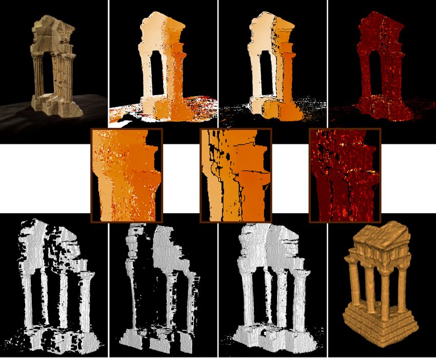
(a) (b) (c) (d)
(e) (f) (g) (h)
Fig. 4: Results of the depth map estimation algorithm. Two neighbouring images
are combined with the reference image (a). If we simply took the NCC peak with the
maximum score, as in [5], we would obtain (b). The result of our algorithm (c) shows a
significant reduction in noise. We have corrected noisy estimates of the surface and the
unknown state has also been used to clearly denote occlusion boundaries and remove
poorly matched regions. The number of the correct surface peak returned, ranked by
NCC score, is displayed in (d) where dark red indicates the peak with the greatest score.
The rendered depth-map is shown in (e) along with the neighbouring depth-map (f ) with
(g) showing the two superimposed. The final reconstruction (h) for the sparse temple
sequence (16 images) of [1]
(a) (b) (c)
Fig. 5: Single view stereo results for the ‘Cones’ data set. The left image of the
stereo pair is shown in (a) with the recovered depth-map in (b), rendered in (c)Using Multiple Hypotheses to Improve Depth-Maps for Multi-View Stereo 13
table provides the accuracy and completeness measures of [1] against the ground-
truth data for the object. In terms of both accuracy and completeness our results
provide a significant improvement in both the sparse ring and ring datasets. In
particular we observe that the results for the sparse ring offer greater accuracy
than the other algorithms [3] running on the ring sequence (3 times as many
images) with the exception of [5].
Accuracy / Completeness
Full (312 images) Ring (47 images) SparseRing (16 images)
Our Results 0.41mm / 99.9% 0.48mm / 99.4% 0.53mm / 98.6%
7 Conclusions
The results of our experiments confirm that our method offers a significant im-
provement in performance over the current state-of-the-art reconstruction algo-
rithms when running on sparse data sets. By explicitly accounting for the failure
modes of the NCC matching technique we are able to produce depth-maps which
accurately locate the true surface in noise, allowing the use of small matching
windows. We are also able to identify when the surface estimate is inconsistent,
due to lack of texture or occlusion, and label pixels as having unknown depths.
Returning this unknown state, rather than providing a form of local regulari-
sation, allows a subsequent global regularisation to be performed over all the
depth-maps using the best possible data. If there are unknown surface regions
which are not recovered by the depth-map a global regularisation scheme is in
a much better position to estimate the surface since it has access to all of the
depth-maps. This is particularly true in the case of the sparse ring temple dataset
and we believe is primarily responsible for its improved performance over other
methods. We also note that our depth-map estimation algorithm may be inte-
grated with a variety of multi-view stereo algorithms [5–7, 12, 17, 18, 21] where
is should confer similar increases in performance.
References
1. Seitz, S., Curless, B., Diebel, J., Scharstein, D., Szeliski, R.: A comparison and
evaluation of multi-view stereo reconstruction algorithms. In: Proc. IEEE Conf.
on Computer Vision and Pattern Recognition. (2006)
2. Scharstein, D., Szeliski, R.: A taxonomy and evaluation of dense two-frame stereo
correspondence algorithms. Intl. Journal of Computer Vision 47(1–3) (2002)
3. http://vision.middlebury.edu/
4. Criminisi, A., Shotton, J., Blake, A., Rother, C., Torr, P.: Efficient dense stereo
with occlusions for new view-synthesis by four-state dynamic programming. Intl.
Journal of Computer Vision 71(1) (2007)
5. Hernández, C., Schmitt, F.: Silhouette and stereo fusion for 3d object modeling.
Computer Vision and Image Understanding 96(3) (December 2004)
6. Vogiatzis, G., Hernández, C., Torr, P.H.S., Cipolla., R.: Multi-view stereo via vol-
umetric graph-cuts and occlusion robust photo-consistency. IEEE Trans. Pattern
Anal. Mach. Intell. 29(12) (2007)14 Neill D.F. Campbell et al.
7. Goesele, M., Curless, B., Seitz, S.: Multi-view stereo revisited. In: Proc. IEEE
Conf. on Computer Vision and Pattern Recognition. (2006)
8. Kolmogorov, V.: Convergent tree-reweighted message passing for energy minimiza-
tion. IEEE Trans. Pattern Anal. Mach. Intell. 28(10) (2006)
9. Hernández, C., Vogiatzis, G., Cipolla, R.: Probabilistic visibility for multi-view
stereo. In: Proc. IEEE Conf. on Computer Vision and Pattern Recognition. (2007)
10. Campbell, N.D.F., Vogiatzis, G., Hernández, C., Cipolla, R.: Automatic 3d ob-
ject segmentation in multiple views using volumetric graph-cuts. In: 18th British
Machine Vision Conference. Volume 1. (2007)
11. Boykov, Y., Kolmogorov, V.: An experimental comparison of min-cut/max-flow
algorithms for energy minimization in vision. IEEE Trans. Pattern Anal. Mach.
Intell. 26(9) (September 2004)
12. Hornung, A., Kobbelt, L.: Hierarchical volumetric multi-view stereo reconstruction
of manifold surfaces based on dual graph embedding. In: Proc. IEEE Conf. on
Computer Vision and Pattern Recognition. (2006)
13. Furukawa, Y., Pons, J.: Accurate, dense, and robust multi-view stereopsis. In:
Proc. IEEE Conf. on Computer Vision and Pattern Recognition. (2007)
14. Vogiatzis, G., Torr, P., Cipolla, R.: Multi-view stereo via volumetric graph-cuts.
In: Proc. IEEE Conf. on Computer Vision and Pattern Recognition. (2005)
15. Habbecke, M., Kobbelt, L.: A surface-growing approach to multi-view stereo re-
construction. In: Proc. IEEE Conf. on Computer Vision and Pattern Recognition.
(2007)
16. Goesele, M., Snavely, N., Curless, B., Hoppe, H., Seitz, S.: Multi-view stereo for
community photo collections. In: Proc. 11th Intl. Conf. on Computer Vision. (2007)
17. Merrell, P., Akbarzadeh, A., Wang, L., Mordohai, P., Frahm, J.-M., Yang, R.,
Nistér, D., Pollefeys, M.: Real-time visibility-based fusion of depth maps. In:
Proc. 11th Intl. Conf. on Computer Vision. (2007)
18. Bradley, D., Boubekeur, T., Heidrich, W.: Accurate multi-view reconstruction us-
ing robust binocular stereo and surface meshing. In: Proc. IEEE Conf. on Computer
Vision and Pattern Recognition. (2008)
19. Hornung, A., Kobbelt, L.: Robust and efficient photoconsistency estimation for
volumetric 3D reconstruction. In: Proc. 9th Europ. Conf. on Computer Vision.
(2006)
20. Sun, J., Li, Y., Kang, S.B., Shum, H.-Y.: Symmetric stereo matching for occlusion
handling. In: Proc. IEEE Conf. on Computer Vision and Pattern Recognition.
(2005)
21. Sinha, S.N., Mordohai, P., Pollefeys, M.: Multi-view stereo via graph cuts on the
dual of an adaptive tetrahedral mesh. In: Proc. 11th Intl. Conf. on Computer
Vision. (2007)
22. Park, J., Kak, A.C.: Multi-peak range imaging for accurate 3D reconstruction of
specular objects. In: Proc 6th Asian Conf. on Computer Vision. (2004)
23. Curless, B., Levoy, M.: A volumetric method for building complex models from
range images. In: Proc. of the ACM SIGGRAPH ‘96. (1996)
24. Zach, C., Pock, T., Bischof, H.: A globally optimal algorithm for robust TV-L1
range image integration. In: Proc. 11th Intl. Conf. on Computer Vision. (2007)
25. Boykov, Y., Kolmogorov, V.: Computing geodesics and minimal surfaces via graph
cuts. In: Proc. 9th Intl. Conf. on Computer Vision. (2003)
26. Woodford, O.J., Reid, I.D., Fitzgibbon, A.W.: Efficient new view syntesis using
pairwise dictionary priors. In: Proc. IEEE Conf. on Computer Vision and Pattern
Recognition. (2007)You can also read