Consistent State Estimation on Manifolds for Autonomous Metal Structure Inspection
←
→
Page content transcription
If your browser does not render page correctly, please read the page content below

Consistent State Estimation on Manifolds
                          for Autonomous Metal Structure Inspection
                 Bryan Starbuck1† , Alessandro Fornasier2† , Stephan Weiss2 , and Cédric Pradalier1

   Abstract— This work presents the Manifold Invariant Ex-
tended Kalman Filter, a novel approach for better consistency
and accuracy in state estimation on manifolds. The robustness
of this filter allows for techniques with high noise potential
like ultra-wideband localization to be used for a wider variety
of applications like autonomous metal structure inspection.
The filter is derived and its performance is evaluated by
testing it on two different manifolds: a cylindrical one and
a bivariate b-spline representation of a real vessel surface,
showing its flexibility to being used on different types of
surfaces. Its comparison with a standard EKF that uses virtual,
noise-free measurements as manifold constraints proves that it
outperforms standard approaches in consistency and accuracy.
Further, an experiment using a real magnetic crawler robot
on a curved metal surface with ultra-wideband localization
shows that the proposed approach is viable in the real world
application of autonomous metal structure inspection.
                                                                   Fig. 1. Simulation of a Magnetic Crawler robot (green circle) on a Ship
                                                                   Hull with an Ultra-wideband Localization Grid (red circles).
                       I. INTRODUCTION
                                                                   space, which can be viewed as a two-dimensional, differen-
   Routine inspection of large metal structures is of the          tiable, Riemannian manifold. This allows us to select a chart
utmost importance in avoiding environmental catastrophe            from the maximum atlas and hence define a chart map, a con-
and maintaining safety standards. Small differential-drive         tinuous, invertible, bijective map, that maps each point of the
robots with magnetic wheels are being deployed on vessels          considered manifold to a two-dimensional Euclidean space.
and cargo ship hulls to ensure that these standards are met,       The full state of the planar robot moving on the manifold is
but as of yet, the task is being completed via manual op-          six-dimensional, including position and orientation within a
eration. Given the expansive dimensions of these structures,       three-dimensional euclidean space, however, its ”planarity”
completing this task autonomously would be preferable, but         gives only three degrees of freedom: a two-dimensional
with such high stakes, having the best localization accuracy       position and the heading angle. Therefore, by applying a
and consistency is paramount. Even though classical methods        consistent IEKF on the product space R2 × SO (2), the
for state estimation exist, they do not consider the fact that     localization problem can be solved entirely on the chart.
the robot is a planar robot moving on a curved surface. Thus,
they tend to estimate the six-dimensional state, enforcing            Being able to evaluate the surface and it’s derivatives at
constraints on all known degrees of freedom, affecting the         any point is necessary to create a basis for the tangent space
consistency of the approach. Therefore, motivated by the           in order to recover the full orientation of the robot from the
recent development of the consistent Invariant Extended            minimal state estimated on the chart. Given that there are no
Kalman Filter (IEKF) [1] [2] [3] [4], in this work, we             equations for generic metal structures like a ship hull, and
propose a Manifold Invariant Extended Kalman Filter, a             that the equation of a surface must be known to apply the
novel approach to consistent state estimation on manifolds         proposed methodology, a bivariate b-spline representation of
with application to ship hull inspection.                          the surface was recognized as a sufficient substitute. This can
                                                                   be obtained by extracting the vertices of the surface from its
   A metal structure, e.g. a ship hull, can be thought of as
                                                                   CAD model for interpolation, or by taking a laser scan of
a smooth surface embedded in three-dimensional Euclidean
                                                                   the structure and interpolating the resulting point cloud.
  This work was supported by the EU-H2020 project BUGWRIGHT2 (GA      The propagation model of the magnetic crawler robot is
871260)                                                            based on its odometry measurements [5], but even with high
  1 Bryan Starbuck and Cédric Pradalier are with Georgia Tech
                                                                   precision wheel encoders, this is only reliable for predicting
Lorraine - CNRS UMI 2958 bstarbuck3@gatech.edu,
cedric.pradalier@georgiatech-metz.fr                               the robot’s state within a plane that is tangent to the surface.
  2 Alessandro    Fornasier     and  Stephan Weiss  are    with    The measurement model for state localization is given by
the   Control     of    Networked    Systems Group,   University   modelling ultra-wideband (UWB) range measurements with
of     Klagenfurt,      Austria     {alessandro.fornasier,         a trilateration framework [6], which in ideal conditions can
stephan.weiss}@ieee.org
  † Theseauthors contributed equally                               accurately update the robot’s position within ±5 cm, but
  Accepted February/2021 for ICRA 2021, DOI follows ASAP ©IEEE.    with high noise potential from wave deflection off the metal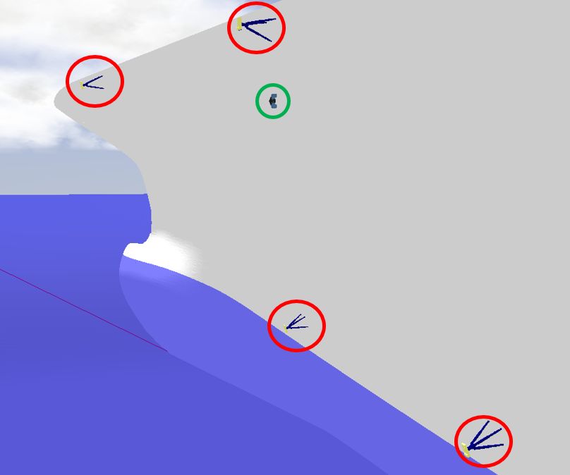
surface, this is not a safe assumption to make [7]. Therefore,
to account for the inherent drifting from the surface that the
robot’s state will experience, classical approaches tend to
solve the localization problem by forcing constraints within
the Extended Kalman Filter (EKF) framework [8]. Imposing
two virtual, zero noise measurements as constraints such
that the first constraint maps the state of the robot to the
surface, and the second one maintains collinearity between
the vertical axis of the robot and the normal to the surface
resulting in a full estimation of the robot’s position and         Fig. 2. Magnetic Crawler Robot (green arrow) on a Curved Metal Surface
orientation, but sacrificing the filter’s consistency. With the    with Ultra-wideband Localization (red circles) and laser (yellow arrow) to
loss of consistency, the loss of accuracy and robustness           track the robot for ground truth.
follows. To validate the benefit and versatility of the proposed   with outdoor applications like metal structure inspection. It
approach compared to classical approaches, simulations were        therefore follows that a grid of UWB beacons for a robot
carried out specifically on cylindrical and curved surfaces,       to localize with respect to could be temporarily installed on
simulating respectively a cylindrical vessel and a ship hull.      the side of a ship hull. Fig. 1 shows a simulation of a ship
Moreover, An experiment with a real magnetic crawler robot         hull with a magnetic crawler robot and four UWB beacons
on a curved metal plate has been performed to show the             in place to form a localization grid.
feasibility of the methodology in real-world scenarios.                Two main factors to consider when developing a filter
                      II. RELATED WORK                             for a problem like this are its accuracy and consistency.
                                                                   It can be difficult to maintain accuracy when using UWB
   Strategies for metal structure inspection can take on many
                                                                   for metal structure inspection due to high noise from wave
forms, but in every case, fundamental questions must be
                                                                   deflection off the metal surface. This error causes a prolonged
investigated, such as: Which sensors should be used for map-
                                                                   time of flight resulting in over-exaggerated range measure-
ping and localization? and, Which filtering technique will
                                                                   ments. Some propose including methods of detecting these
produce the best results? For bridge inspection, unmanned
                                                                   divergences by analysing the noise distribution to decide
aerial vehicles (UAVs) equipped with lidar for mapping and
                                                                   if a measurement is usable [13]. Others suggest loosely or
visual, inertial odometry systems for localization collect data
                                                                   tightly coupled filters to resolve the problem [14]. A loosely
from the bridge to be processed for structural analysis [9].
                                                                   coupled, two step update of orientation correction followed
For ship hull inspection, autonomous underwater vehicles
                                                                   by position correction can give good results, although it
(AUVs) equipped with cameras for mapping and sonar sys-
                                                                   is said that a tightly coupled measurement model, where
tems for localization similarly complete the task [10]. How-
                                                                   position and orientation are corrected at the same time can
ever, it should be noted that the inspection of metal structures
                                                                   better overcome large positioning errors [15]. Even when
and vessels is not solely confined to airborn inspection or to
                                                                   using tightly coupled EKFs to achieve higher accuracy,
below the waterline. In fact, large cargo ships can protrude
                                                                   there is still the likelihood of inconsistency in this case
up to and exceeding fifty meters above water level espe-
                                                                   due to the aforementioned problem related to the robot’s
cially when unloaded. Therefore, to complete the inspection
                                                                   planarity being expressed with six degrees of freedom. This
most efficiently and in it’s entirety, utilizing a combination
                                                                   can cause the covariance of the robot’s state to become
of UAVs, AUVs, and differential-drive, magnetic-wheeled
                                                                   disproportionately small resulting in an overconfidence in
crawler robots could be quite advantageous.
                                                                   the propagation and eventually a divergence to an incorrect
   The crawlers hold primary responsibility for inspecting
                                                                   solution [16]. As Manifold filters solve this problem, they
the portion of the ship hull that protrudes from the water,
                                                                   have proven themselves to be more consistent, and more
and high accuracy localization is fundamental to this being
                                                                   accurate on average, than other filters [17]. The Invariant
accomplished autonomously. There are various sensors that
                                                                   filter formulation [1] [2] [3] is proven to solve the afore-
come to mind as candidates for correcting the position of
                                                                   mentioned problems by ensuring the Log-Linear property of
the robot such as RTK-GPS, Wifi, and UWB. RTK-GPS is
                                                                   the error, that is, the independence of the error dynamics
too unreliable given that clear line of sight to satellites is
                                                                   from the state estimate. We employed the Invariant filter
always required, and Wifi is also unreliable because it is too
                                                                   formulation within a manifold-based space showing that our
sensitive to interference. UWB which is based on the time of
                                                                   Manifold Invariant Extended Kalman Filter (M-IEKF) results
flight of wave transmission resulting in a range measurement
                                                                   in greater consistency and improved accuracy.
is proven to be a reliable method of localizing multiple
moving targets [11]. The major factor which highlights                                     III. T HEORY
UWB as a more robust method for this application is that             In this section, a general understanding of differential
it has high bandwidth meaning that the waves experience            geometry, manifolds, and bivariate b-spline surface repre-
less interference while reliably transmitting small packets of     sentations is introduced.
data at a distance generally up to 30 meters [12]. Although
UWB is generally used for indoor object tracking, given that       A. Manifolds
more specialized filters are being developed to enhance its          An n-dimensional manifold M is a topological space
robustness, it is becoming increasingly feasible to experiment     (M, Θ) with the property that each point p ∈ M has a
neighborhood that is homeomorphic to the Euclidean space
Rn . Thus, if ∀ p ∈ M, ∃ U ∈ Θ | σ : U 7→ σ (U) ⊂ Rn for
which the following conditions hold:
          σ is invertible, thus ∃ σ −1 : σ (U) 7→ U         (1)
          σ is continuous                                   (2)
          σ −1 is continuous                                (3)

   Then (U, σ) is called a chart at (M, Θ) and
σ : U 7→ σ (U) ⊂ Rn is called a chart map.
   Although there are different classifications of manifolds,
differentiable manifolds are of primary focus along this work,
because this type of manifold allows a globally differentiable
tangent space, shown in Fig. 3, to be defined using calculus.
For each point p ∈ M, the tangent space Tp M is the space
formed by the collection of all tangent vector velocities that     Fig. 3. Illustration of a manifold M, the tangent space Tp M at p ∈ M
a curve γ (t) passing through p may have. More formal              and its basis vectors {B1 (p) , B2 (p) , N (p)}.
definitions and a more detailed introduction of the tangent
space can be found in [18].                                        computed at p as follows:
                                                                                                                        T
                                                                        L3 (p) = Dx φ (x, y, z)         Dy φ (x, y, z) −1           (9)
                                                                                    L3 (p)
                                                                         N (p) =                                                   (10)
B. Surfaces                                                                       kL3 (p)k
                                                                      Furthermore, for any given surface, or in other words,
   Considered smooth surfaces embedded in R3 ,                     for any considered manifold, we can choose a chart and
which in practice would cover almost all encountered               hence a continuous, differentiable, and invertible chart map
vessel     surfaces,    are    2-Dimensional      parallelizable   σ : M → R2 which maps points from the manifold to a
manifolds M = {(x, y, z) ∈ R3 | φ (x, y, z) = 0}, where            euclidean space of a dimension equal to dim (M).
φ : R3 → R is a scalar function that imposes a constraint
that defines the shape of the surface. A manifold is called        C. Spline Interpolation
parallelizable if there exists a smooth vector field {B1 , B2 },
such that for every point p ∈ M, the tangent vectors                  Bivariate b-splines, which are piecewise polynomial func-
{B1 (p) , B2 (p)} provide a basis of the tangent space Tp M        tions can fit a variety of complex shapes while maintaining
at p. Within these surfaces being considered are explicit          continuity in their derivatives. This surface representation
surfaces, where one of its variables can be solved for given       can be evaluated at any point, and being a polynomial, the
the constraint imposed by φ (x, y, z) = 0 (e.g. a paraboloid),     derivatives are easily obtained, making it sufficient to create
and implicit surfaces which are described by an implicit           a basis for the tangent space so that the manifold properties
equation φ (x, y, z), where one of its variables cannot be         and constraints can be applied in the state estimation. The
solved for (e.g. a cylinder). However, any given surface           surface is defined as follows:
embedded in R3 can always be written in its implicit                                             k X
                                                                                                 X l

form φ (x, y, z) = 0, where the zeros of the constraint are                         f (x, y) =             Bxi Byj cij             (11)
the points p ∈ M of the surface. Therefore, the basis                                            i=1 j=1
of the tangent space Tp M at p, and thus the manifold              The coefficients cij are determined from the vertices being
parallelization, can be defined as follows:                        interpolated. The b-splines Bx and By are determined from
                                             T                   their endpoints, known as knots, in each respective dimen-
               V1 (p) = 1 0 Dx φ (x, y, z)                   (4)
                                             T                   sion, for each piecewise polynomial. Then, the coefficients
               V2 (p) = 0 1 Dy φ (x, y, z)                   (5)   are multiplied by the tensor product of the b-splines resulting
                                                                   in a surface [19].
   Although this way of defining the parallelization is per-
fectly valid, it is not the only admissible one, and, as shown                           IV. METHODOLOGY
in Fig. 3, one can also choose a parallelization which forms
an orthonormal basis of the tangent space Tp M at p:                  In this section, the general problem of state estimation
                                                                   for a wheeled robot moving on a smooth surface and a
  L1 (p) = Dx φ (x, y, z) V2 (p) − Dy φ (x, y, z) V1 (p) (6)       detailed description of the adopted methodology to solve
  L2 (p) = Dx φ (x, y, z) V1 (p) + Dy φ (x, y, z) V2 (p) (7)       this problem is introduced, followed by the experimental
            L1 (p)                 L2 (p)                          procedure that was carried out. This includes the process of
  B1 (p) =              B2 (p) =                         (8)       charting the manifold and applying an M-IEKF to a minimal
           kL1 (p)k               kL2 (p)k
                                                                   state represented on the product space between the chosen
  Then, the normal vector to the tangent space Tp M can be         chart and SO (2), or directly on SE (2).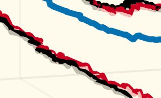
the tangent space, then we can compute:
∆xk ∆b1k
∆yk = B1 (pk ) B2 (pk ) N (pk ) ∆b2k (16)
∆zk 0
The robot position projected on the manifold can then be
easily computed through the chosen chart map as follows:
uk
= σ (xk + ∆xk , yk + ∆yk , zk + ∆zk ) (17)
Fig. 4. Illustration of stereographic projection leveraged to define a vk
continuous, differentiable and invertible chart map on the cylinder.
It is important to note that if the velocity vector (or
T
dispacement vector) [∆b1 ∆b2] on the tangent space Tp M
The key to implementing the methodology is to first find at p is affected by gaussian noise, the linearity of the mapping
a chart that covers the whole manifold being considered, and in Eq. (16) will allow its gaussianity to be preserved.
hence find a continuous, differentiable chart map σ (p), and If a minimal state representation given by
its inverse σ −1 (u, v). X = (t, R (θ)) = (u, v, R (θ)) ∈ R2 × SO (2) on the
Let us first consider the easiest case of an explicit, smooth product space between the chosen chart and SO (2), where
surface described by an explicit function where one of the the rotation defined by SO (2) is the rotation of the robot
variables involved is solved for. For example, z = f (x, y). about its own vertical axis, thus its heading, then an IEKF
In this case, for every p ∈ M, the chart map and its inverse can be designed following algorithm 1.
are simply determined as follows: In the case of the ship hull simulation, the same method-
ology is applied to a bivariate b-spline representation of the
u x surface. The vertices are extracted from the CAD model of
σ (p) = σ (x, y, z) = = (12)
v y the ship and interpolated. In the case of the real metal plate
x u experiment, the vertices are taken from a laser scan of the
σ −1 (u, v) = p = y = v (13) surface before the experiment is carried out, and the point
z f (u, v) cloud is interpolated. Fig. 2 shows the magnetic crawler robot
attached to the curved metal surface that was used, with a
In the most difficult case of implicit, smooth surfaces, a UWB beacon attached to it (a tag), and another in the corner
chart, and hence a chart map covering the whole manifold (an anchor). Only one anchor is shown, but In total there
needs to be defined without having a simple and predefined were four. The laser was also used during the experiment to
recipe to apply. Consider a cylinder of radius R and height track the robot for ground truth. The robot collects four tag-
h as a possible manifold to cover with a chart. As a first to-anchor ranges at a time and uses trilateration to compute
solution, mapping every point of the cylinder to a plane by its position as a measurement in the update function of the
unwrapping the cylinder seems logical, however, this solution M-IEKF algorithm.
will result in discontinuities at the border of the map at 2π.
V. EXPERIMENTS
Instead, the stereographic projection can be leveraged to find
a continuous, differentiable chart map, shown in Fig. 4, and A. Evaluation
defined as follows: In this section, the performance of the M-IEKF is eval-
" xh # uated first by testing it on a cylindrical manifold to show
u
σ (p) = σ (x, y, z) = = exp(z) yh (14) its ability to work with any surface that is a parallelizable
v exp(z) manifold and to simulate the case of a cylindrical vessel.
√ Ru The M-IEKF is then compared to a standard filter (MC-
x u2 +v 2
EKF) that uses two virtual, zero noise measurements to keep
Rv
σ −1 (u, v) = y = √ (15)
u2 +v2 the state constrained on the curved surface. Moreover, as
z log √uRh a proof of concept for metal structure inspection, we have
2 +v 2
tested the M-IEKF on a simulated ship hull showing that
Once a chart covering the manifold has been found, an the proposed methodology can handle the case of a priori
IEKF is applied on a space which is partially defined by not-known surface obtained by bivariate b-spline intepolation
the chosen chart and then lifted back to all the estimated from known points on the surface. Finally, the real world vi-
results on the manifold. In order to do so, first, a mapping ability of the M-IEKF in metal structure inspection is shown
that allows us to map a velocity vector (or displacement with an experiement employing a magnetic wheeled crawler
T
vector) [∆b1 ∆b2] on the tangent space Tp M at p to a robot on a curved metal surface. In this last experiment, the
T
velocity vector (or displacement vector) [∆x ∆y ∆z] on R3 triangulated position of the robot was availabe via UWB
must be found. Then, the chosen chart map must be used to measurements.
project the robot position to the chart. In general, if a wheeled For the two simulated tests, a Monte-Carlo simulation
robot is moving on a manifold and pk = {xk , yk , zk } ∈ M of N = 100 trials was run. We computed the Root Mean
is the position of the robot at a given time step k, and Squared Error (RMSE) in position and orientation, further-
T
[∆b1k ∆b2k ] ∈ Tp M is the linear displacement vector in more, the Average Normalized Estimation Error Squared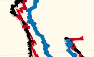
Algorithm 1: IEKF on the product space R2 ×SO (2)
+
Input: X̂ k−1 , P̂+
k−1 , ∆bk , ∆θk , yk
Propagation
// Map estimate
−1
onto M
p̂+
k−1 = σ t̂+
k−1
// Robot rotation Ck−1 in R3
Bk−1 = [B1 (pk−1 ) B2 (pk−1 ) N (pk−1 )]
R (θk−1 ) 0
Ck−1 = Bk−1 T
0 1
// Map deltas from Tp M to R3
∆pk = Ck−1 ∆bk
// Projection onto the chart Fig. 5. Ground-truth (in black) and estimated trajectory (in red) of the
t̂− +
M-IEKF on a cylindrical surface. Note the wrong initialization of the filter.
k = σ p̂k−1 + ∆pk
// IEKF
rotation
propagation
R θ̂k− = R θ̂k−1
+
Exp (∆θk )
// Jacobians
∂σ (σ −1 (tk−1 ))
Fk = ∂tk−1
t̂+
k−1
1
" #
∂σ(pk )
∂(pk )
Ck−1
Gk = p̂+
k−1
+∆pk
1
// Covariance propagation
Σ∆bk
P̂− + T
k = Fk P̂k−1 Fk + Gk
T
σ∆θk Gk
2
End
Update
// Residual
−
rk = h X̂ k − yk
// Jacobian
Hk = ∂h(X)
∂X +
X̂ k
// Kalman gain
−1
Kk = P̂− T − T
k Hk Hk P̂k Hk + Σy k
// IEKF Update Fig. 6. M-IEKF full state RMSE and ANEES averaged over 100 runs
t̂+
k = t̂
k + δtk corresponding to the estimation problem on the cylindrical surface.
R θ̂k+ = Exp (δθk ) R θ̂k
The RMSE gives an indication of how far the esti-
−
P̂+
k = (I − Kk Hk ) P̂k mate varies from the ground truth on average, whereas the
End
ANEES, which is normalized by the covariance of the filter
Output: X̂ k , P̂k
at each time step, gives a standard for whether a filter is a
credible estimator. The closer to 1 an estimator is within the
probability interval, the more credible it is, and therefore the
more consistency the filter has [20] [21].
(ANEES) were computed for each time step, averaged over
the N trials, and compared between the two filters. The B. Results
aforementioned metrics are defined as follows: Fig. 5 and 6 show the trajectory and the error metrics
respectively for the M-IEKF during the cylinder manifold
simulation. The trajectory plot shows that the state estimate
s
PN
i=1 e2ik follows closely with the ground truth which is also cor-
RM SE = (18)
N roborated by the error metrics. The RMSE for the heading
is mostly below 0.01 rad, and the RMSE for its position
N
1 X T −1 are predominantly below 10 cm in each dimension giving
AN EES = e P ei (19) a good indication that the filter can perform accurately.
N m i=1 ik ik k
Furthermore, the ANEES is almost completely confined to
where eik and Pik are respectively the estimation error and the probability interval, and it is centered about 1 indicating
the error covariance for the i-th run at a given time step k. that the filter is credible and consistent. To further evaluate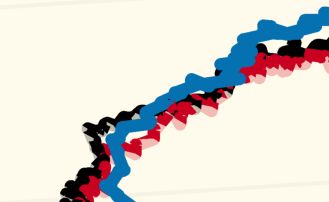
Fig. 7. Ground-truth (in black) and estimated trajectory of the M-IEKF     Fig. 8. Ground-truth of the magnetic crawler robot (in black) and estimated
and the MC-EKF (respectively in red and blue) on a b-spline interpolated   trajectory of the M-IEKF and the MC-EKF (respectively in red and blue).
surface corresponding to the curved surface of a ship hull.                Dots (in green) correspond to the position measurements from the UWB
                                                                           trilateration. Note the cyan circle showing the failure of the MC-EKF on
                                                                           providing an estimate that is not attached to the surface.

the filter, Fig. 7 and 9 show the trajectory and the error
metrics respectively for the M-IEKF and the MC-EKF during
the ship hull simulation. The trajectory plot shows that the
state estimate of the M-IEKF follows closely with the ground
truth like it did in the cylinder experiment, whereas the MC-
EKF clearly starts diverging. The error metrics show that
the M-IEKF still performs consistently and accurately, but
with a little bit more error in comparison with the error in
the cylinder simulation which was expected considering that
its state is being estimated on an interpolated surface this
time. By contrast, the MC-EKF shows significantly higher
error in the RMSE for its position up to 50 cm in some
instances in the x direction, and the ANEES plot clearly
shows that it goes outside of the probability interval and is
therefore not consistent. Fig. 8 shows the trajectory from
the real experiment on the curved metal plate for each filter
along with the UWB measurements, and Fig. 10 shows
the position RMSE for each filter. The M-IEKF follows
quite closely to the ground truth, only having noticeable
error when there is a high concentration of erroneous UWB
measurements due to the metal surface deflection which can
be seen near time step 625. The MC-EKF does not follow
closely to the ground truth as expected with errors up to                  Fig. 9. Comparison between MC-EKF and M-IEK in terms of position
80 cm. The results back up the fact that the M-IEKF is                     RMSE and ANEES corresponding to the case of b-spline interpolated
                                                                           surface.
consistent and more accurate than standard approaches like
the MC-EKF, allowing further extensions like the inclusion
of a measurement update rejection test, making it a viable
option for consistent and robust metal structure inspection
with ultra-wideband localization.
                        VI. CONCLUSION
   The Manifold Invariant Extended Kalman Filter is a novel
approach for consistent state estimation on manifolds. It
combines manifold state representation and invariance to
achieve greater consistency and accuracy. We proved that the
proposed M-IEKF is applicable to a wide range of vessel
surfaces encountered in real world applications. Further,
we showed results validating that the M-IEKF outperforms                   Fig. 10. Position RMSE of the M-IEKF and MC-EKF (in red and blue
classical approaches when using real robot wheel odometry                  respectively) corresponding to the real magnetic crawler robot experiment.
and UWB measurements. Therefore, the M-IEKF makes
metal structure inspection with ultra-wideband localization
viable.
R EFERENCES
[1] A. Barrau and S. Bonnabel, “The invariant extended kalman filter as
a stable observer,” IEEE Transactions on Automatic Control, vol. 62,
no. 4, pp. 1797–1812, 2016.
[2] ——, “An ekf-slam algorithm with consistency properties,” arXiv
preprint arXiv:1510.06263, 2015.
[3] ——, “Invariant kalman filtering,” Annual Review of Control,
Robotics, and Autonomous Systems, vol. 1, no. 1, pp. 237–257, 2018.
[Online]. Available: https://doi.org/10.1146/annurev-control-060117-
105010
[4] E. Allak, A. Fornasier, and S. Weiss, “Consistent covariance pre-
integration for invariant filters with delayed measurements,” in 2020
IEEE/RSJ International Conference on Intelligent Robots and Systems
(IROS). IEEE, 2020.
[5] S. Thrun, “Probabilistic robotics,” Communications of the ACM,
vol. 45, no. 3, pp. 52–57, 2002.
[6] M. Mirbach, “A simple surface estimation algorithm for uwb pulse
radars based on trilateration,” in 2011 IEEE International Conference
on Ultra-Wideband (ICUWB). IEEE, 2011, pp. 273–277.
[7] D. Gao, A. Li, and J. Fu, “Analysis of positioning performance of
uwb system in metal nlos environment,” in 2018 Chinese Automation
Congress (CAC). IEEE, 2018, pp. 600–604.
[8] A. J. Trevor, J. G. Rogers, C. Nieto, and H. I. Christensen, “Applying
domain knowledge to slam using virtual measurements,” in 2010 IEEE
International Conference on Robotics and Automation. IEEE, 2010,
pp. 5389–5394.
[9] S. Jung, S. Song, S. Kim, J. Park, J. Her, K. Roh, and H. Myung, “To-
ward autonomous bridge inspection: A framework and experimental
results,” in 2019 16th International Conference on Ubiquitous Robots
(UR). IEEE, 2019, pp. 208–211.
[10] M. S. B. M. Soberi and M. Z. B. Zakaria, “Autonomous ship hull
inspection by omnidirectional path and view,” in 2016 IEEE/OES
Autonomous Underwater Vehicles (AUV). IEEE, 2016, pp. 38–43.
[11] S. Lan, C. Yang, B. Liu, J. Qiu, and A. Denisov, “Indoor real-time
multiple moving targets detection and tracking using uwb antenna ar-
rays,” in 2015 International Symposium on Antennas and Propagation
(ISAP). IEEE, 2015, pp. 1–4.
[12] R. Zetik, O. Hirsch, and R. Thoma, “Kalman filter based tracking of
moving persons using uwb sensors,” in 2009 IEEE MTT-S Interna-
tional Microwave Workshop on Wireless Sensing, Local Positioning,
and RFID. IEEE, 2009, pp. 1–4.
[13] L. Cheng, H. Chang, K. Wang, and Z. Wu, “Real time indoor
positioning system for smart grid based on uwb and artificial intel-
ligence techniques,” in 2020 IEEE Conference on Technologies for
Sustainability (SusTech). IEEE, 2020, pp. 1–7.
[14] J. Clemens and K. Schill, “Extended kalman filter with manifold state
representation for navigating a maneuverable melting probe,” in 2016
19Th International Conference On Information Fusion (FUSION).
IEEE, 2016, pp. 1789–1796.
[15] H. Benzerrouk and A. Nebylov, “Robust imu/uwb integration for
indoor pedestrian navigation,” in 2018 25th Saint Petersburg Interna-
tional Conference on Integrated Navigation Systems (ICINS). IEEE,
2018, pp. 1–5.
[16] B. B. Ready, “Filtering techniques for pose estimation with applica-
tions to unmanned air vehicles,” 2012.
[17] M. Brossard, A. Barrau, and S. Bonnabel, “A code for un-
scented kalman filtering on manifolds (ukf-m),” arXiv preprint
arXiv:2002.00878, 2020.
[18] P.-A. Absil, R. Mahony, and R. Sepulchre, Optimization algorithms
on matrix manifolds. Princeton University Press, 2009.
[19] C.-J. Li and R.-H. Wang, “Bivariate cubic spline space and bivariate
cubic nurbs surfaces,” in Geometric Modeling and Processing, 2004.
Proceedings. IEEE, 2004, pp. 115–123.
[20] X. R. Li, Z. Zhao, and V. P. Jilkov, “Practical measures and test
for credibility of an estimator,” in Proc. Workshop on Estimation,
Tracking, and Fusion—A Tribute to Yaakov Bar-Shalom. Citeseer,
2001, pp. 481–495.
[21] X. R. Li, Z. Zhao, and X. B. Li, “Evaluation of Estimation Algo-
rithms: Credibility Tests,” IEEE Transactions on Systems, Man, and
Cybernetics Part A: Systems and Humans, vol. 42, no. 1, pp. 147–163,
2012.You can also read