Deep SIMBAD: Active Landmark-based Self-localization Using Ranking -based Scene Descriptor
←
→
Page content transcription
If your browser does not render page correctly, please read the page content below
Deep SIMBAD:
                                           Active Landmark-based Self-localization Using Ranking -based Scene Descriptor

                                                                                                     Tanaka Kanji

                                           Abstract— Landmark-based robot self-localization has re-             deep-learning extension. In pattern recognition, SIMBAD is
                                        cently garnered interest as a highly-compressive domain-                a highly-compressive method to describe an object as its
                                        invariant approach for performing visual place recognition              dissimilarities from r prototypes (e.g., r = 500), which is
arXiv:2109.02786v1 [cs.RO] 6 Sep 2021

                                        (VPR) across domains (e.g., time of day, weather, and season).
                                        However, landmark-based self-localization can be an ill-posed           particularly effective when traditional vectorial descriptions
                                        problem for a passive observer (e.g., manual robot control), as         of objects are difficult to obtain or inefficient for learning.
                                        many viewpoints may not provide an effective landmark view.             We adopt SIMBAD because of the following two reasons:
                                        In this study, we consider an active self-localization task by          (1) First, the landmark selection problem is analogous to
                                        an active observer and present a novel reinforcement learning           and can be informed by the well-investigated problem of
                                        (RL)-based next-best-view (NBV) planner. Our contributions
                                        are as follows. (1) SIMBAD-based VPR: We formulate the prob-            prototype selection or optimization [8]. (2) Second, many
                                        lem of landmark-based compact scene description as SIMBAD               recent deep learning techniques can effectively measure
                                        (similarity-based pattern recognition) and further present its          the (dis)similarity between an object and prototypes [9],
                                        deep learning extension. (2) VPR-to-NBV knowledge transfer:             instead of directly describing an object. However, the deep
                                        We address the challenge of RL under uncertainty (i.e., active          learning extension of SIMBAD has not yet been sufficiently
                                        self-localization) by transferring the state recognition ability
                                        of VPR to the NBV. (3) NNQL-based NBV: We regard the                    investigated, and hence is the main focus of our current study.
                                        available VPR as the experience database by adapting nearest-              Most existing self-localization techniques reported hith-
                                        neighbor approximation of Q-learning (NNQL). The result                 erto assume a passive observer (e.g., manual robot control)
                                        shows an extremely compact data structure that compresses               and do not consider the issue of viewpoint planning or
                                        both the VPR and NBV into a single incremental inverted
                                                                                                                observer control. However, landmark-based self-localization
                                        index. Experiments using the public NCLT dataset validated
                                        the effectiveness of the proposed approach.                             can be an ill-posed problem for a passive observer, as many
                                                                                                                viewpoints may not provide an effective landmark view.
                                                               I. I NTRODUCTION                                 Therefore, we aim to develop an active observer that can
                                           Landmark-based robot self-localization has recently gar-             adapt its viewpoints, thereby avoiding non-salient scenes that
                                        nered interest as a highly-compressive domain-invariant ap-             provide no effective landmark view, or moving efficiently
                                        proach for performing visual place recognition (VPR) across             toward locations that are the most informative, to reduce
                                        domains (e.g., time of day, weather, season). In long-term              sensing/computation costs. This is associated closely with the
                                        cross-domain navigation [1]–[3], a robot vision must be able            NBV problem investigated in machine vision studies [10].
                                        to recognize its location (i.e., self-localization) and the main        However, in our cross-domain scenario, the NBV planner
                                        objects [4] (i.e., landmarks) in the scene. This landmark-              is trained and tested in different domains. The cost for
                                        based self-localization problem presents two unique chal-               retraining such an NBV planner that does not consider
                                        lenges. (1) Landmark selection: In the offline training stage,          domain shifts is high in cross-domain scenarios, and we
                                        the robot must learn the main landmarks that represent the              intend to address this issue in the current study.
                                        robot workspace in either a self-supervised or unsupervised
                                        manner [5]. (2) Next best view (NBV): In the online self-
                                        localization stage, the robot must determine the NBVs to
                                        re-identify as many spatially sparse landmarks as possible
                                        [6]. This study focuses on the NBV problem.
                                           In landmark-based self-localization, the only available
                                        feature (Fig. 1) in each map/live scene x is landmark pi (i ∈
                                        [1, r]) observed at signal strength d(x, pi ) (i.e., landmark
                                        ID + intensity). This is in contrast to many existing self-
                                        localization frameworks that assume the availability of vec-            Fig. 1. Motivation. Unlike existing approaches that maintain the model of
                                        torial features for each map image. To address this issue, we           an entire environment (left panel), we aim to maintain only a small fraction
                                        formulate the landmark-based self-localization as similarity-           (i.e., landmark regions) of the robot workspace (right panel). Hence, the per-
                                                                                                                domain cost for retraining (change detection, map updating) is inherently
                                        based pattern recognition (SIMBAD) [7] and present its                  low. However, self-localization with such spatially sparse landmarks can
                                                                                                                be an ill-posed problem for a passive observer, as many viewpoints may
                                           Our work has been supported in part by JSPS KAKENHI Grant-in-Aid     not provide an effective landmark view. Therefore, we considered an
                                        for Scientific Research (C) 17K00361 and 20K12008.                      active observer and presented an active landmark-based self-localization
                                           The authors are with Graduate School of Engineering, University of   framework.
                                        Fukui, Japan. tnkknj@u-fukui.ac.jp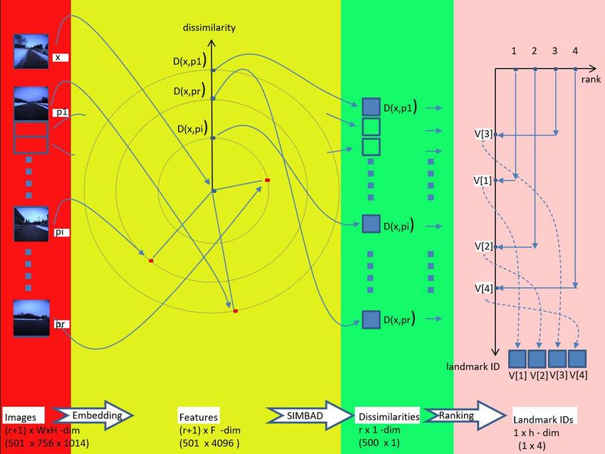
In this study, we investigated an active landmark-based                     modules exist, i.e., landmark selection, mapping, and nearest-
self-localization framework from a novel perspective of SIM-                   neighbor Q-learning, which operates offline to learn the
BAD. Our primary contributions are threefold: (1) SIMBAD-                      prior knowledge (“landmarks,” “map,” and “Q-function”)
based VPR: First, we present a landmark-based compact                          required for the abovementioned three main modules. These
scene descriptor by introducing a deep-learning extension of                   individual modules are described in detail in the following
SIMBAD. Our strategy is to describe each map/live scene                        subsections.
x with dissimilarities {d(x, pi )} from the prototypes (i.e.,
landmarks) {pi }ri=1 and further compress it into a length h                   A. Landmark Model
(≪ r) list of ranked IDs (e.g., r = 500, h = 4) of top-h most                      The proposed landmark model can be explained as fol-
similar landmarks {(v1 , · · · , vh )|d(x, pv1 ) < · · · < d(x, pvh )},        lows. Let R = {p1 , p2 , · · · , pr } be a set of r predefined
which can then be efficiently indexed using an inverted                        prototypes (i.e., landmarks). For a dissimilarity measure d,
index. (2) VPR-to-NBV knowledge transfer: Second, we                           which measures the dissimilarity between a prototype p
address the challenge of RL under uncertainty (i.e., active                    and an input object x, one may consider a new description
self-localization) by transferring the state recognition ability               based on the proximities to the set R, as D(x, R) =[d(x, p1 ),
of VPR to the NBV. Our scheme is based on a recently                           d(x, p2 ), · · ·, d(x, pr )]. Here, D(x, R) is a data-dependent
developed method of reciprocal rank feature (RRF) [11],                        mapping D(·, R): X → Rr from a representation X to the
inspired by our previous works [11]–[13], which is effective                   dissimilarity space, defined by set R. This is a vector space, in
for transfer learning [14] and information retrieval [15]. (3)                 which each dimension corresponds to a dissimilarity D(·, pi )
NNQL-based NBV: Third, we regard the available VPR                             to the prototype from R. A vector D(·, pi ) of dissimilarities
as the experience database by adapting nearest-neighbor                        to the prototype pi can be interpreted as a feature. It is
approximation of Q-learning (NNQL) [16]. The result is                         noteworthy that even when no landmark is present in the
an extremely compact data structure that compresses the                        input image, the proposed model still can describe the image
VPR and NBV into a single incremental inverted index.                          as dissimilarities to the landmarks.
Experiments using the public NCLT dataset validated the                            The advantage of this representation is its applicability to
effectiveness of the proposed approach.                                        any method in dissimilarity spaces, including recent deep
                                                                               learning techniques. For example, d can be (1) a pairwise
                            II. A PPROACH                                      comparison network (e.g., deep Siamese [17]) that predicts
   The active self-localization system aims to estimate the                    the dissimilarity d(x, p) between p and x, (2) a deep anomaly
robot location on a prelearned route (Fig. 2). It iterates for                 detection network (e.g., deep autoencoder [18]) that predicts
each viewpoint, three main steps: scene description, (passive)                 the deviation d(x|p) of x from learned prototypes p, (3) an
self-localization, and NBV planning. The scene description                     object proposal network (e.g., feature pyramid network [19])
describes an input map/live image x as its dissimilarities                     that predicts object bounding-boxes and class label d(p|x)
D(x, ·) from the predefined landmarks. The (passive) self-                     (e.g., [20]), (4) an L2 distance | f (x) − f (p)| of deep feature
localization incorporates each perceptual/action measure-                       f (·) [21] between p and x, as well as (5) any methods
ment into the belief of the robot viewpoint. The NBV                           for dissimilarities d(p, x) including those for non-visual
planning takes the scene descriptor x of a live image and
determines the NBV action. In addition, three additional

                                                                               Fig. 3. Scene description module. First, the input query/landmark images
Fig. 2. Active self-localization system. Online processing comprised three     are translated into vectorial features. Subsequently, the query feature is
main stages: scene description, passive self-localization, and NBV planning.   described by its dissimilarities from the landmark features. Next, the
Offline processing comprised landmark selection, mapping, and NN Q-            dissimilarity values are ranked to obtain a ranked list of top-h most similar
learning. Details of the scene description module are provided in Fig. 3.      landmarks. Finally, the proposed landmark ranking-based scene descriptor
Details of the NN lookup module are provided in Fig. 4.                        is obtained.
modalities (e.g., natural language). In the current study, the         element is the reciprocal 1/v[i] of the rank value v[i] of the
experimental system was based on (4) using NetVLAD [22]                i-th landmark if v[i] ≤ h, or 0 otherwise. For more details
as the feature extraction network f (·). We believe that this          regarding the RRF, please refer to [11].
enables effective exploitation of the discriminative power of             During the active multi-view self-localization, the results
a deep neural network within SIMBAD.                                   of (passive) self-localization at each viewpoint are incre-
                                                                       mentally integrated by a particle filter (PF). PF is a com-
B. Landmark Selection                                                  putationally efficient implementation of a Bayes filter, and
   The landmark selection is performed prior to the train-             can address multimodal belief distributions [25]. In the PF-
ing/testing phase, in an independent “landmark domain”.                based inference system, the robot’s 1D location on the route
Landmarks should be selected such that they are dissimilar             prelearned in the training domain is regarded as the state.
to each other. This is because, if the dissimilarity d(pi , p j ) is   The PF system is initialized at the starting viewpoint of the
small for a prototype pair, d(x, pi ) ≃ d(x, p j ) for other objects   robot. In the prediction stage, the particles are propagated
x, then either pi or p j is a redundant prototype. Intuitively,        through a dynamic model using the latest action of the
an ideal clustering algorithm may identify good landmarks              robot. In the update stage, the likelihood models for the
as cluster representatives. However, this clustering is NP-            landmark observation are approximated by the RRF, and the
hard [23]. In practice, heuristics such as k-means algorithms          weight of each k-th particle is updated as wk ←wk +vRRF [uk ],
are often used as alternatives. Moreover, the utility issue            where vRRF [uk ] is the RRF element that corresponds to the
(e.g., [24]) complicates the problem, i.e., landmark visibility        hypothesized viewpoint uk . Other details are the same as that
and other observation conditions (e.g., occlusions and field-          of the PF-based self-localization framework [25].
of-views) must be considered to identify useful landmarks.
For such landmark selection, only a heuristic approximate              D. NBV Planning
solution exists, i.e., no analytical solution exists [5].                 The NBV planning task is formulated as an RL prob-
   In our study, we do not focus on the landmark selection             lem, in which a learning agent interacts with a stochastic
method; instead, we propose a simple and effective method.             environment. The interaction is modeled as a discrete-time
Our solution comprises three procedures: (1) First, high-              discounted Markov decision process (MDP). A discounted
dimensional vectorial features X = {x} (i.e., NetVLAD)                 MDP is a quintuple (S, A, P, R, γ ), where S and A are the set
are extracted from individual candidate images. (2) Sub-               of states and actions, P the state transition distribution, R the
sequently, each candidate image x ∈ X is scored by the                 reward function, and γ ∈ (0, 1) a discount factor (γ = 0.9).
dissimilarity minx′ ∈X\{x} |x − x′ | from its nearest neighbor         We denote by P(·|s, a) and R(s, a) the probability distribution
over the other features. (3) Finally, all the candidate images         over the next state and the immediate reward of performing
are sorted in the descending order of the scores, and the              action a at state s, respectively.
top-r images are selected as the prototype landmarks. This                A Markov policy is the distribution over the control actions
approach offers two advantages. First, the selected landmarks          for the state, in our case represented by the scene descriptor
are expected to be dissimilar to each other. In addition, the          of a live image (i.e., s = x). The action-value function of
dissimilarity features D(·, R) are expected to become accurate         a policy π , denoted by Q : S × A → R, is defined as the
when the robot approaches a viewpoint with landmark view.              expected sum of discounted rewards that are encountered
                                                                       when policy π is executed. For an MDP, the goal is to
C. Self-localization
                                                                       identify a policy that yields the best possible values, Q∗ (s, a)
   The (offline) mapping is performed prior to the self-               = supπ Qπ (s, a), ∀(s, a) ∈ S × A.
localization tasks, in an independent “training domain”. It
extracts a 4,096 dim NetVLAD image feature from each
map image x and then translates it to an r-dim dissimilarity
descriptor D(x, ·). Subsequently, it sorts the r elements of the
descriptor in the ascending order and returns an ordered list
of top-h ranked landmark IDs, which is our proposed h-dim
scene descriptor (Fig. 3). With an inverted index, the map
image’s ID is indexed by using its landmark ID and the rank
value, as primary and secondary keys (Fig. 4).
   The (online) self-localization is performed in a new “test
domain”. It translates an input query image to a ranking-
based descriptor. Subsequently, the inverted index is looked           Fig. 4.    Nearest neighbor scheme. (1) Offline mapping stage: First, a
                                                                       map image is translated to a landmark ranking-based scene descriptor.
up using each landmark ID in the ordered list as a query.              Subsequently, the image ID is inserted into the inverted index entries that
Hence, a short list of map images with a common landmark               have common landmark IDs. (2) Online self-localization stage: First, a
ID is obtained. Next, the relevance of a map image is                  live image is translated into a landmark ranking-based scene descriptor.
                                                                       Next, a shortlist is obtained from the inverted index entries that have
evaluated as the inner product hvrRRF (q), vhRRF (m)i of RRF           common landmark IDs, and then refined. Finally, the viewpoints or Q-values
between the query image q and each map image m in the                  associated with the nearest neighbor states are obtained from the experience
short list. An RRF vhRRF is an r-dim h-hot vector whose i-th           database, and then returned.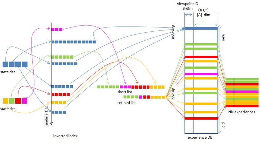
40
The implementation of the “Q-function” Q(·, ·) as a
computationally tractable function is a key issue. A naive 35
implementation of the function Q(·, ·) is to employ a two- 30
dimensional table, which is indexed by a state-action pair
(s, a) and whose element is a Q-value [26]. However, this 25
ANR [%]
simple implementation presents several limitations. In par- 20 brute-force
SIMBAD
ticular, it requires a significant amount of memory space, bag of landmarks
RRF
15
proportional to the number and dimensionality of the state
vectors, which are intractable in many applications including 10
ours. An alternative approach is to use a deep neural network 5
based approximation of the Q-table (e.g., DQN [27]), as in
0
[28]. However, the DQN must be retrained for every new
WI-
WI-
SP
SP
SU
SU
AU
AU
-S
-A
-
-
-
-
SP
SU
AU
WI
WI
SP
U
U
domain with a significant amount of space/time overhead. train-test
(a)
Herein, we present a new highly efficient NNQL-based
50
approximation that reuses the existing inverted index (II-C) bag-of-landmarks
SIMBAD
to approximate Q(·, ·) with a small additional space cost. RRF
Our approach is inspired by the recently developed 45
nearest-neighbor approximation of the Q-function (Fig. 4)
[16]. Specifically, the inverted index which was originally 40
developed for VPR (II-C) is regarded as a compressed repre-
sentation of visual experiences in the training domain. Recall
35
that the inverted index aims to index map image ID using
the landmark ID. Next, we now introduce a supplementary
two-dimensional table called “experience database” that aims 30
to index action-specific Q-values Q(s, ·) by map image ID.
Subsequently, we approximate the Q-function by the NNQL 25
2 4 6 8 10 12 14 16 18 20
[16]. The key difference between NNQL and the standard rank list length
(b)
Q-learning is that the Q-value of an input state-action pair Fig. 6. ANR performance of VPR.
(s, a) in the former is approximated by a set of Q-values
that are associated with its k nearest neighbors (k = 4). Next, We used the publicly available NCLT dataset [29]. The
we used the supplementary table to store the action-specific data we used included view image sequences along vehicle
Q values Q(s, ·). Hence, the Q-function is approximated by trajectories acquired using the front-facing camera of the
|N(s|a)|−1 ∑(s′ ,a)∈N(s|a) Q(s′ , a), where N(s|a) is the nearest Ladybug3, as well as ground-truth GPS viewpoint informa-
neighbor of (s, a) conditioned on a specified action a. In tion. Both indoor and outdoor change objects such as cars,
fact, such an action-specific NNQL can be regarded as an pedestrians, construction machines, posters, and furniture
instance of RL. For more details regarding NNQL, please were present during seamless indoor and outdoor navigation
refer to [16]. by the Segway robot.
In the experiments, we used four different datasets, i.e.,
III. E XPERIEMENTS “2012/1/22 (WI)”, “2012/3/31 (SP)”, “2012/8/4 (SU)”, and
“2012/11/17 (AU)”, which contained 26,208, 26,364, 24,138,
We evaluated the effectiveness of the proposed algorithm and 26,923 images (Fig. 5). They were used to create
via self-localization tasks in a cross-season scenario. eight different landmark-training-test domain triplets (Fig.
2): WI-SP-SU, WI-SP-AU, SP-SU-AU, SP-SU-WI, SU-AU-
WI, SU-AU-SP, AU-WI-SP, and AU-WI-SU. The number of
landmarks was set to 500 for every triplet, which is consistent
with the settings in our previous studies using the same
dataset (e.g., [30]).
For NNQL training, the learning rate was set α = 0.1. Q-
value for a state-action pair was initialized to 0.0001, and a
positive reward of 100 was assigned when the belief value of
the ground-truth viewpoint was top-10% ranked. The number
of training episodes was 10,000. The action candidates are a
set of forward movements A = {1, 2, · · ·, 10} [m] along the
route defined in the NCLT dataset. One episode consists of
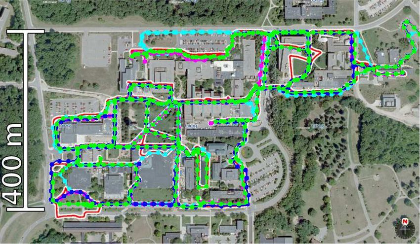
Fig. 5. Experimental environments. The trajectories of the four datasets,
“2012/1/22”, “2012/3/31”, “2012/8/4”, and “2012/11/17”, used in our
an action sequence of length 10, and its starting location is
experiments are visualized in green, purple, blue, and light-blue curves, randomly sampled from the route.
respectively. The VPR performance at each viewpoint in the context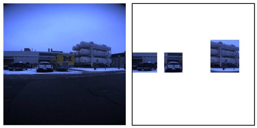
above was measured based on the averaged normalized                                    the other two methods have as bad VPR performance as the
rank (ANR). In the ANR, a subjective VPR is modeled                                    chance method (i.e., ANR=50%).
as a ranking function that takes an input query image and                                 Figure 7 demonstrates the performance of active self-
assigns a rank value to each map image. Subsequently, the                              localization. Note that each episode has a different number of
rank values for the ground-truth map images are computed,                              valid observations, and long episodes do not always provide
normalized by the number of map images, and averaged over                              high performance. We plot the ANR performance for all
all test queries, thereby yielding the ANR. A VPR system                               test images (frames) on the graph in Fig. 7, regardless of
with high ANR performance can be regarded as having                                    how many episodes were observed. In the figure, “proposed”
nearly perfect performance and high retrieval robustness [31],                         is the performance of NBV using NNQL trained using the
which is typically required in loop closing applications [32].                         RRF feature as a state vector. “baseline” is different from
   Four different scene descriptors based on NetVLAD were                              “proposed” only in that the action is randomly determined.
developed as the baseline/ablation methods: “brute-force”,                             “a[m]” (a ∈ [1, 10]) is a naive strategy that repeats the same
“SIMBAD”, “bag-of-(most-similar-)landmarks”, and “RRF”.                                forward movement a[m] at every viewpoint, independent of
In “brute-force”, the map model is a nearest-neighbor search                           the RRFs. They often performed worse than the “proposed”,
based on the L2 dissimilarity measure with NetVLAD of the                              and to make the matters worse, which action is best is
query image, assuming that every map image is described                                domain-dependent and cannot be known in advance. The
by the NetVLAD feature. In the other three methods, the                                characteristics that the higher the VPR performance, the
map model describes each map image by the dissimilarities                              better the active self-localization performance, is consistent
with the h most similar landmarks. More specifically, “bag-                            with our recent studies dealing with other VPR methods
of-landmarks” assumes h-hot binary (0/1) similarity value,                             (e..g, pole-landmark-based VPR [28], e.g., convolutional
“SIMBAD” uses the h-hot L2 dissimilarity value, and “RRF”                              neural network -based VPR [33], and e.g., map-matching-
uses the h-hot RRF similarity value.                                                   based VPR [34]). It is noteworthy that the proposed method
   It is noteworthy that the three methods “SIMBAD”, “bag-                             outperformed all the methods considered here, although the
of-landmarks”, and “RRF” require significantly lower time                              landmark-based VPR and NNQL-based NBV were com-
cost owing to the availability of efficient inverted index.                            pressed into a single incremental inverted index.
   In terms of space cost, “bag-of-landmarks” is the most                                 Finally, we also investigated the space/time performance.
efficient, “RRF” and “SIMBAD” are slightly more expensive                              The inverted index consumes 15h-bit per map image. The
because they need to memorize the rank value for each                                  main processes, extracting NetVLAD features, VPR, and
map image, and “brute-force” is intractably expensive as it                            NBV consumes 8.6 ms (GPU), 495.4 ms (CPU), and
requires to memorize the high-dimensional map features.                                7×10⁻³ ms (CPU) per viewpoint (CPU: intel core i3-1115G4
   Figure 6 shows ANR of single-view VPR tasks.                                        3.00GHz). The most time consuming part is the scene
   As can be seen from Fig. 6 (a), the “brute-force” method                            description processing in VPR, which consumes 410 ms.
shows very good recognition performance, but at the cost of                            The NBV is significantly fast, compared with the recent deep
high time/space cost for per-domain retraining. As we found                            learning variants, thus the additional cost for the extension
in [11], NetVLAD’s utility as a dissimilarity-based feature                            from the passive to active self-localization was little.
vector is low. In this experiment, the method “SIMBAD”
was about the same as “bag-of-landmarks” and had slightly                                    IV. C ONCLUSIONS     AND   F UTURE D IRECTIONS
lower performance. Compared with these two methods, the                                   Herein, a new framework for active landmark-based self-
proposed method “RRF” had much higher performance.                                     localization for highly compressive applications (e.g., 40-bit
To summarize, the proposed method “RRF” achieves a                                     image descriptor) was proposed. Unlike previous approaches
good trade-off between time/space efficiency and recognition                           of active self-localization, we assumed the main landmark
performance. In subsequent experiments, we will use this                               objects as the only available model of the robot’s workspace
“RRF” as the default method for the passive self-localization                          (“map”), and proposed to describe each map/live scene as
module.                                                                                dissimilarities to these landmarks. Subsequently, a novel re-
   As can be seen from Fig. 6 (b), in the case where the rank                          ciprocal rank feature-based VPR-to-NBV knowledge transfer
list length (i.e., descriptor size) is very small (e.g., h = 4),                       was introduced to address the challenge of RL under un-
the proposed method has a small performance drop, while                                certainty. Furthermore, an extremely compact data structure
          50                                                           1 [m]
                                                                       2 [m]           that compresses the VPR and NBV into a single incremental
          45                                                           3 [m]
                                                                       4 [m]
                                                                       5 [m]
                                                                                       inverted index was presented. The proposed framework was
          40                                                           6 [m]
                                                                       7 [m]
                                                                       8 [m]
                                                                                       experimentally verified using the public NCLT dataset.
          35
                                                                       9 [m]
                                                                                          Future work must investigate how to accelerate the
ANR [%]

                                                                      10 [m]
          30                                                        baseline

          25
                                                                   proposed            (dis)similarity evaluator d(·, ·) while retaining the ability
          20
                                                                                       to discriminate between different levels of (dis)similarities.
          15
                                                                                       In the training phase, the evaluator is repeated for every
          10
                                                                                       viewpoint of every episode. Since the number of repetitions
               WI-SP   WI-SU   SP-SU   SP-AU       SU-AU
                                           train-test
                                                           SU-WI     AU-WI     AU-SP
                                                                                       is very large (e.g., 10,000×10×500=5×10⁷), efficiency of
                 Fig. 7.   Performance results for active self-localization.           calculation is the key to suppress per-domain retraining
cost. Another direction for future research is compression [19] S.-W. Kim, H.-K. Kook, J.-Y. Sun, M.-C. Kang, and S.-J. Ko, “Parallel
of the proposed scene/state descriptor, towards extremely- feature pyramid network for object detection,” in Proceedings of the
European Conference on Computer Vision (ECCV), 2018, pp. 234–
compressive applications (e.g., [35]). Although the proposed 250.
ranking-based descriptor is the first compact (e.g., 40-bit) de- [20] S. Hanada and K. Tanaka, “Partslam: Unsupervised part-based scene
scriptor for the VPR-to-NBV applications, it is still uncom- modeling for fast succinct map matching,” in 2013 IEEE/RSJ Inter-
national Conference on Intelligent Robots and Systems. IEEE, 2013,
pressed, i.e., it may be further compressed. Finally, our on- pp. 1582–1588.
going research topic is to incorporate various (dis)similarity [21] A. Babenko, A. Slesarev, A. Chigorin, and V. Lempitsky, “Neural
evaluators into the proposed deep SIMBAD framework, codes for image retrieval,” in European conference on computer vision.
Springer, 2014, pp. 584–599.
including non-visual -based (dis)similarity evaluators (II-A). [22] R. Arandjelovic, P. Gronat, A. Torii, T. Pajdla, and J. Sivic, “Netvlad:
Cnn architecture for weakly supervised place recognition,” pp. 5297–
5307, 2016.
R EFERENCES [23] K. Tanaka, “Self-supervised map-segmentation by mining minimal-
map-segments,” in 2020 IEEE Intelligent Vehicles Symposium (IV).
[1] M. J. Milford and G. F. Wyeth, “Seqslam: Visual route-based nav- IEEE, 2020, pp. 637–644.
igation for sunny summer days and stormy winter nights,” in 2012 [24] K. Tanaka, H. Zha, and T. Hasegawa, “Viewpoint planning in map
IEEE International Conference on Robotics and Automation, 2012, updating task for improving utility of a map,” in Proceedings 2003
pp. 1643–1649. IEEE/RSJ International Conference on Intelligent Robots and Systems
[2] W. Churchill and P. Newman, “Experience-based navigation for long- (IROS 2003)(Cat. No. 03CH37453), vol. 1. IEEE, 2003, pp. 729–734.
term localisation,” The International Journal of Robotics Research, [25] F. Dellaert, D. Fox, W. Burgard, and S. Thrun, “Monte carlo localiza-
vol. 32, no. 14, pp. 1645–1661, 2013. tion for mobile robots,” in 1999 International Conference on Robotics
[3] R. Arroyo, P. F. Alcantarilla, L. M. Bergasa, and E. Romera, “Fusion and Automation (ICRA), vol. 2, 1999, pp. 1322–1328.
and binarization of cnn features for robust topological localization [26] R. S. Sutton, A. G. Barto, et al., Introduction to reinforcement
across seasons,” in 2016 IEEE/RSJ International Conference on Intel- learning. MIT press Cambridge, 1998, vol. 135.
ligent Robots and Systems (IROS), 2016, pp. 4656–4663. [27] J. Fan, Z. Wang, Y. Xie, and Z. Yang, “A theoretical analysis of deep
[4] A. Torralba, K. P. Murphy, W. T. Freeman, and M. A. Rubin, “Context- q-learning,” in Learning for Dynamics and Control. PMLR, 2020,
based vision system for place and object recognition,” in Computer pp. 486–489.
Vision, IEEE International Conference on, vol. 2. IEEE Computer [28] K. Tanaka, “Active cross-domain self-localization using pole-like
Society, 2003, pp. 273–273. landmarks,” in 2021 IEEE International Conference on Mechatronics
[5] M. Bürki, C. Cadena, I. Gilitschenski, R. Siegwart, and J. Nieto, and Automation (ICMA), 2021, pp. 1188–1194.
“Appearance-based landmark selection for visual localization,” Journal [29] N. Carlevaris-Bianco, A. K. Ushani, and R. M. Eustice, “University
of Field Robotics, pp. 4137–4143, 2016. of michigan north campus long-term vision and lidar dataset,” The
[6] S. K. Gottipati, K. Seo, D. Bhatt, V. Mai, K. Murthy, and L. Paull, International Journal of Robotics Research, vol. 35, no. 9, pp. 1023–
“Deep active localization,” IEEE Robotics and Automation Letters, 1035, 2016.
vol. 4, no. 4, pp. 4394–4401, 2019. [30] T. Hiroki and K. Tanaka, “Long-term knowledge distillation of visual
[7] A. Feragen, M. Pelillo, and M. Loog, Similarity-Based Pattern Recog- place classifiers,” in 2019 22st International Conference on Intelligent
nition: Third International Workshop, SIMBAD 2015, Copenhagen, Transportation Systems (ITSC), 2019.
Denmark, October 12-14, 2015. Proceedings. Springer, 2015, vol. [31] P. Hiremath and J. Pujari, “Content based image retrieval using color,
9370. texture and shape features,” in 15th International Conference on
[8] K. S. Gurumoorthy, P. Jawanpuria, and B. Mishra, “Spot: A framework Advanced Computing and Communications (ADCOM 2007). IEEE,
for selection of prototypes using optimal transport,” arXiv preprint 2007, pp. 780–784.
arXiv:2103.10159, 2021. [32] J. P. Company-Corcoles, E. Garcia-Fidalgo, and A. Ortiz, “Lipo-
[9] B. Li, W. Wu, Q. Wang, F. Zhang, J. Xing, and J. Yan, “Siamrpn++: lcd: Combining lines and points for appearance-based loop closure
Evolution of siamese visual tracking with very deep networks,” in detection.” in BMVC, 2020.
Proceedings of the IEEE/CVF Conference on Computer Vision and [33] K. Kurauchi and K. Tanaka, “Deep next-best-view planner for cross-
Pattern Recognition, 2019, pp. 4282–4291. season visual route classification,” in 2020 25th International Confer-
[10] M. Mendoza, J. I. Vasquez-Gomez, H. Taud, L. E. Sucar, and C. Reta, ence on Pattern Recognition (ICPR), 2021, pp. 497–502.
“Supervised learning of the next-best-view for 3d object reconstruc- [34] K. Tanaka, “Active map-matching: Teacher-to-student knowledge
tion,” Pattern Recognition Letters, vol. 133, pp. 224–231, 2020. transfer from visual-place-recognition model to next-best-view planner
[11] K. Takeda and K. Tanaka, “Dark reciprocal-rank: Teacher-to- for active cross-domain self-localization,” in 2021 IEEE International
student knowledge transfer from self-localization model to graph- Conference on Computational Intelligence and Virtual Environments
convolutional neural network,” in 2021 International Conference on for Measurement Systems and Applications (CIVEMSA), 2021, pp. 1–
Robotics and Automation (ICRA), 2021, pp. 4348–4355. 6.
[12] K. Tanaka, “Detection-by-localization: Maintenance-free change ob- [35] F. Yan, O. Vysotska, and C. Stachniss, “Global localization on
ject detector,” in 2019 International Conference on Robotics and openstreetmap using 4-bit semantic descriptors,” in 2019 European
Automation (ICRA). IEEE, 2019, pp. 4348–4355. Conference on Mobile Robots (ECMR). IEEE, 2019, pp. 1–7.
[13] ——, “Unsupervised part-based scene modeling for visual robot
localization,” in 2015 IEEE International Conference on Robotics and
Automation (ICRA). IEEE, 2015, pp. 6359–6365.
[14] G. Hinton, O. Vinyals, and J. Dean, “Distilling the knowledge in a
neural network,” arXiv preprint arXiv:1503.02531, 2015.
[15] P. K. Atrey, M. A. Hossain, A. El Saddik, and M. S. Kankanhalli,
“Multimodal fusion for multimedia analysis: a survey,” Multimedia
systems, vol. 16, no. 6, pp. 345–379, 2010.
[16] D. Shah and Q. Xie, “Q-learning with nearest neighbors,” arXiv
preprint arXiv:1802.03900, 2018.
[17] Y. Zhan, K. Fu, M. Yan, X. Sun, H. Wang, and X. Qiu, “Change
detection based on deep siamese convolutional network for optical
aerial images,” IEEE Geoscience and Remote Sensing Letters, vol. 14,
no. 10, pp. 1845–1849, 2017.
[18] J. An and S. Cho, “Variational autoencoder based anomaly detection
using reconstruction probability,” Special Lecture on IE, vol. 2, no. 1,
pp. 1–18, 2015.You can also read