Machine Learning to Improve Multi-hop Searching and Extended Wireless Reachability in V2X
←
→
Page content transcription
If your browser does not render page correctly, please read the page content below
IEEE COMMUNICATIONS LETTERS, VOL. 00, NO. 00, MARCH 2020                                                                                       1

 Machine Learning to Improve Multi-hop Searching
   and Extended Wireless Reachability in V2X
               Manuel Eugenio Morocho-Cayamcela , Member, IEEE, Haeyoung Lee , Member, IEEE,
                                      and Wansu Lim , Member, IEEE

   Abstract—Multi-hop relay selection is a critical issue in vehicle-         might not be always ideal. A better approach would be to
to-everything networks. In previous works, the optimal hopping                minimize the propagation loss along the entire multi-hop path
strategy is assumed to be based on the shortest distance. This                by recognizing the location of the obstructions that attenuate
study proposes a hopping strategy based on the lowest propaga-
tion loss, considering the effect of the environment. We use a two-           the signal, and avoiding transmission through them.
step machine learning routine: improved deep encoder-decoder                     Recent wireless communications and artificial intelligence
architecture to generate environmental maps and Q-learning to                 efforts have investigated the recognition of the patterns in
search for the multi-hopping path with the lowest propagation
                                                                              these obstructions [4]. Before adopting deep learning (DL),
loss. Simulation results show that our proposed method can
improve environmental recognition and extend the reachability                 researchers used decision-tree based approaches such as texton
of multi-hop communications by up to 66.7%, compared with a                   forests with low accuracy results [5]. These days, convolutional
shortest-distance selection.                                                  neural networks (CNNs) have increased the segmentation
   Index Terms—Machine learning, multi-hop wireless communi-                  performance significantly. Patch-based segmentation classifies
cation, Q-learning, vehicle-to-everything.                                    the entire image using a collection of small patches [6]. A
                                                                              major drawback of using patches is that the classification
                      I. I NTRODUCTION                                        network is composed of connected layers requiring fixed
                                                                              size images. To overcome this limitation, designs based on
      EHICLE to everything (V2X) networks constitute auto-
V     mobiles and involve entities that act as wireless nodes for
exchanging standardized information. This data is transmitted
                                                                              fully-convolutional networks (FCNs) use a pre-trained CNN
                                                                              to serve as a down-sampling encoder, and then up-sample
                                                                              the features using fractional-stride convolution [7]. However,
using one-way or two-way dedicated short-range communica-
                                                                              this up-sampling approach introduces information loss and
tion (DSRC), which are specifically designed wireless com-
                                                                              generates coarse segmentation maps [8]. Moreover, these DL
munication channels that correspond to a set of protocols and
                                                                              models have not been exploited before to improve multi-hop
standards [1]. Mechanisms such as intelligent multi-hop relay
                                                                              selection by detecting obstructions in satellite imagery.
selection and route searching are interesting and challenging
methods of extending the communication over a large area.                        In this paper, we propose a two-step machine learning
For further enhancement of DSRC, researchers have looked                      (ML) process to improve multi-hop relay selection and extend
into several areas including the improvement of reachabil-                    wireless reachability in a NLOS V2X network.
ity (currently limited to approximately 300 m) [2]. Previous                  •   First, we segment satellite images into different classes
works based the design of multi-hop search algorithms in the                      (i.e., buildings, open fields, and streets). To achieve this,
minimization of the Euclidean distance to the destination [3].                    we modify SegNet [8], a pretrained CNN encoder-decoder
Nevertheless, a real non-line-of-sight (NLOS) V2X scenario                        by updating its parameters according to the exponentially
includes obstructions where the shortest-distance hopping                         weighted average of the gradients. Our approach solves the
   Manuscript received November 12, 2020; revised December 14 2019;               coarse map problem, accelerates segmentation convergence,
accepted March 19, 2020. Date of publication March 31 2020; date of current       and increases accuracy as compared to FCNs.
version March 31 2020.
   This work was supported by the National Research Foundation of Korea
                                                                              •   Second, we use the map generated by our segmentation
(NRF) under grant 2017R1C1B5016837, in part by the Information Technol-           network to assign a reward and penalty when transmission
ogy Research Center (ITRC) Project Group under grant IITP-2019-2014-1-            is done by a vehicle via a path with low propagation loss,
00639, in part by Kumoh National Institute of Technology (2019-104-155),
and in part by the European Union’s Horizon 2020 research and innovation
                                                                                  and a high propagation loss obstruction, respectively. Our
programme 5G-HEART project under grant 857034.                                    method enables the transmitting vehicle to learn an optimal
   M. E. Morocho-Cayamcela is with the Department of Electronic Engi-             hopping policy by maximizing the cumulative reward.
neering, Kumoh National Institute of Technology, Gumi, Gyeongsangbuk-do,
39177 South Korea. e-mail: (eugeniomorocho@kumoh.ac.kr).                      From the results in the first stage of our proposal, the obstacles
   H. Lee is with the 5G Innovation Centre (5GIC), Institute for Communica-
tion Systems (ICS), University of Surrey, Guildford, GU2 7XH U.K. (e-mail:    recognition accuracy increases by an average of 3.04% when
haeyoung.lee@surrey.ac.uk)                                                    compared with FCNs. Results from the second stage show
   W. Lim is with the Department of IT Convergence Engineering, Kumoh         that the reachability of a V2X link can be extended by
National Institute of Technology, Gumi, Gyeongsangbuk-do, 39177 South
Korea. e-mail: (wansu.lim@kumoh.ac.kr).                                       approximately 66.7% using our multi-hop selection policy
   Digital Object Identifier                                                  compared with the shortest-distance strategy.

                      1558-2558 c 2019 IEEE. Personal use is permitted, but republication/redistribution requires IEEE permission.
                                    See https://www.ieee.org/publications/rights/index.html for more information.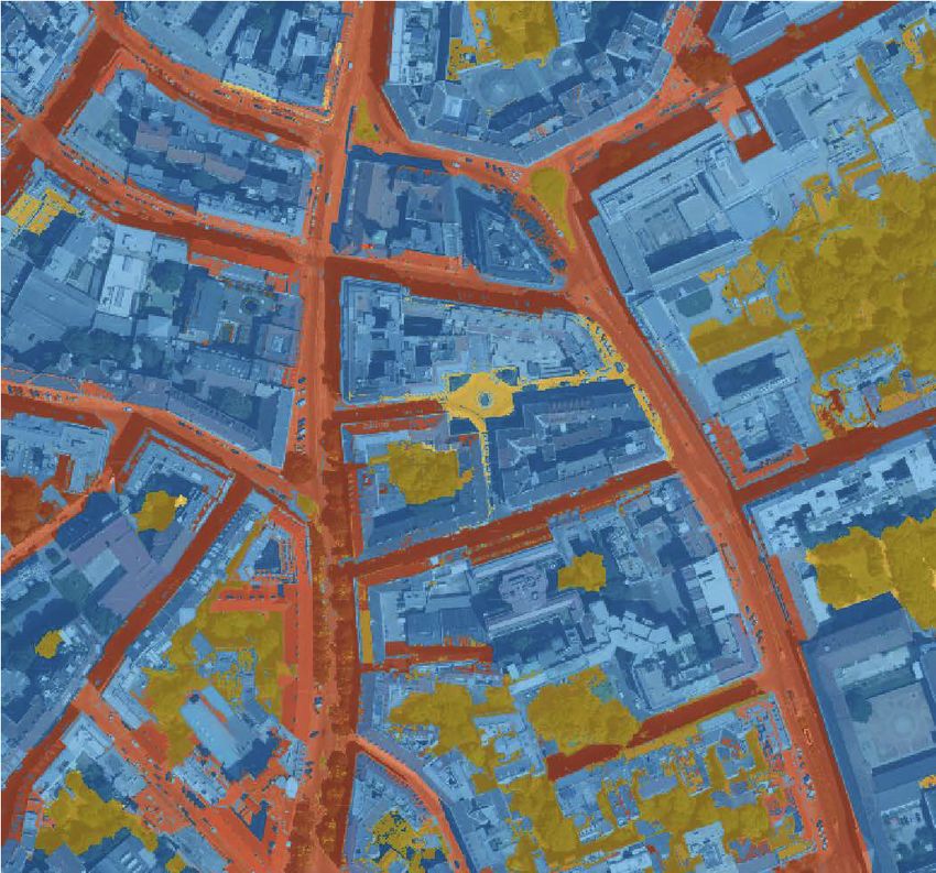
2                                                                                IEEE COMMUNICATIONS LETTERS, VOL. 00, NO. 00, MARCH 2020

    II. A DDRESSING THE REACHABILITY LIMITATION WITH                   indices are recalled from the corresponding encoder layer to
                   M ACHINE L EARNING                                  decode lower resolution feature maps. Non-linear up-sampling
   The first stage of our proposal involves enhancing a con-           improves boundary delineation and reduces the number of
volutional encoder-decoder to detect obstacles that might              parameters for training [8]. The network is initialized using
block or attenuate the signal (section II-A). The second stage         the weights of the pre-trained VGG-16 model [11], to exploit
presents an off-policy model-free algorithm to find the multi-         transfer learning by dropping the last fully-connected layers
hop path with the lowest propagation loss, extending V2X               and replacing them with the categories in c. If we let f
reachability (section II-B). The model assumes: 1) massive             be our network parametrized by θ, the segmentation output
machine-type communications (mMTC) scenarios with a large              of the network is M = f (X, θ), where M ∈ R5000×5000 is
number of devices spread geographically, and 2) no prior               a categorical matrix that maps every pixel from the input
knowledge of the propagation loss between devices.                     image to the corresponding category in c. Our network is
                                                                       trained by updating θ iteratively, moving the loss towards the
                                                                       minimum of the cost function J(θ). The cost function measures
A. Obstruction Detection in Satellite Imagery                          the pixel-wise performance of our model prediction against
   To recognize obstructions, a DL network is trained to               its corresponding ground truth. To quantify the difference
segment three types of classes (i.e., buildings, open fields,          between the two distributions, we let J(θ) be defined as
and streets) from aerial images. We use the INRIA aerial               the pixel-wise cross-entropy, because it penalizes the model
image dataset to train our algorithm [9]. INRIA is a collec-           when it estimates a low probability for a target category,
tion of high-resolution imagery from different European and            producing larger gradients and converging faster [12]. For
American landscapes (e.g., Austin, Bellingham, Bloomington,            our multi-class segmentation problem with K = |c| = 3
Chicago, Colorado, Innsbruck, Kitsap County, San Francisco,            number of categories, and a training set with the values of
East Tyrol, and Vienna). The dataset contains 180 color images         (X (i), Y (i) ) for i ∈ {1, . . . , mtr }, we find the set of parameters
of 5000 × 5000 pixels, covering a surface of 1500 m × 1500 m           θ = {θ (1), . . . , θ (n) } that minimizes J(θ) by computing a per-
each. As opposed to [9], [10], we generate a ground truth              example loss L(X, Y, θ) = − log p(Y |X; θ) for each category
map on top of INRIA by labelling every pixel in each of                k ∈ c, on every pixel-wise observation and sum the outcomes
the 180 images with one of our environmental categories                as follows:
in c = {buildings, open fields, streets}. We let each image                                            1 Õ
                                                                                                            mtr ÕK

X (i) ∈ R5000×5000 be a matrix of 5000 × 5000 pixels. The set                              J(θ) = −                L(X (i), Y (i), θ)
                                                                                                      mtr i=1 k=1
of m images on INRIA as X , {X (1), . . . , X (m) }, where each                                                                             (1)
                                                                                                            mtr ÕK
pixel in X (i) can be mapped to one of the categories in c.                                            1 Õ           (i)

                                                                                                                               (i)
                                                                                                  =−               Y log p̂k ,
Y (i) ∈ R5000×5000 is used to present the corresponding ground-                                       mtr i=1 k=1 k
truth map. Similarly, we can express Y , {Y (1), . . . , Y (m) }
for its corresponding set of labels. Labeling was conducted            where Y (i)
                                                                                 k
                                                                                    represents the desired output for the i th instance on
according to the following criteria:                                   class k, and p̂(i)
                                                                                       k
                                                                                          represents the estimated probability that the i th
• Buildings: include residential areas, and any field where the        instance belongs to k. Because the optimization of θ involves
   signal might be blocked by man-made structures.                     calculating the derivative of J(θ) through partial differential
• Open fields: include parks, and any open area where the              equations, we can write the gradient vector of (1) with respect
   signal might be blocked by sparse vegetation.                       to θ (k) as follows:
• Streets: include highways, or wherever a line of sight                                                    mtr
                                                                                                    1       Õ
   between the transmitter and receiver can be guaranteed.                            ∇θ (k) J(θ) =     ∇θ        L(X (i), Y (i), θ)
                                                                                                    mtr     i=1
The dataset was augmented by applying random left/right                                                  mtr                           (2)
reflection, and X/Y translation to the images with a ±10                                            1 Õ          (i)     (i)

                                                                                                  =            p̂ − Y k X .     (i)
pixels range. After dataset augmentation, majority of the pixels                                    mtr i=1 k
correspond to the ‘buildings’ class. This imbalance biases the
                                                                       Note that each class has its own dedicated parameter vector
learning process in favor of the dominant class. To overcome
                                                                       θ (k) , that constructs the parameter matrix θ. To find the local
this challenge, the classes are balanced by computing the in-
                                                                       minimum of J(θ), we take steps proportional to the negative
verse frequencies, where the class weights are set to the inverse
                                                                       of the gradient of (2) for every i. The process is initiated by
of their frequencies. This method increases the weight given to
                                                                       estimating an initial θ, and iteratively updating its value to
the under-represented classes (i.e., ‘open field’, and ‘street’).
                                                                       reduce the value of the cost function.
After the pixel-wise labeled dataset [X : Y ] is balanced, the
                                                                           Considering the training instances in the dataset may
dataset is divided into training set [X tr : Y tr ] and testing set
                                                                       scale to a size where the optimization of θ may
[X te : Y te ]. Fig. 1(a) illustrates how the convolutional encoder-
                                                                       be computationally        prohibitive,     we  sample a minibatch
decoder takes an input image X (i) through convolution, batch                                          0           0
                                                                       B = X (1) : Y (1) , . . . , X (mt r ) : Y (mt r ) , and let the opti-

normalization, ReLu, and pooling layers to build the down-
                                                                       mization algorithm follow the gradient g downhill with:
sampling encoder. The encoder is followed by an up-sampling
                                                                                                        m0
network with reverse architecture, where the max pooling                                     1    Õ tr

                                                                                         g ← 0 ∇θ      L(X (i), Y (i), θ)                  (3)
                                                                                            mtr   i=1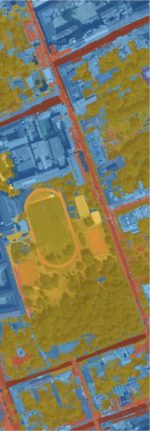
MOROCHO-CAYAMCELA et al.: MACHINE LEARNING TO IMPROVE MULTI-HOP SEARCHING AND EXTENDED WIRELESS REACHABILITY IN V2X 3
Input Convolutional Encoder-Decoder Output Street
St t Street
reeet
Open Field
ld Open Field
ld Street
RGB Image
I S
Segmentation
t ti RSU3 RSU4
Pooling Indices
Policy $ Open Field
ld Open Field St
Street Buildings Street
Agent
Buildings "!+1 V1 Street Street
ett V4
!
Open Field #!+1 Buildings
gs Str
Street
Stre
Street Environment Street
Stre
St reet
re et RSU1
Buildingss Buildings Street Buildingss Open Field
Pixel-wise Cross Entropy
RSU2
Conv. + Batch. Norm. + ReLU Pooling Upsampling
samp
mpling
mp ng So
Soft
Softmax
ftma
max Acti
max Activation
tiva
va
vati Street Street
Street
Stre
tree
eet
V2 V3 St
Street
St Street
et
(a) (b)
Fig. 1. Proposed system architecture. (a) Our convolutional encoder-decoder takes an aerial image as its input, and outputs a pixel-wise categorical matrix
containing semantic information for each pixel. (b) The agent vehicle V1 takes a transmitting action At on the environment and receives a reward Rt at
state St . The action of the vehicle is taken based on a wireless transmission policy π. For the following iterations, V1 receives a reward Rt +1 and the state
changes to St +1 . V1 learns an optimal transmission policy by maximizing the cumulative reward.
θ ← θ − βg, (4) Algorithm 1 Parameter optimization and image segmentation
Input: T Xlat , T Xlon , RXlat , RXlon , m, k, K, x, y, learning rate β,
where β is a positive value that determines the size of each momentum η, initial parameter θ, initial velocity v, Rb , Ro , Rs .
step in the minimization process, known as learning rate. A Output: Categorical matrix M.
limitation of updating θ with (4), is that the created oscillations Initialization:
1: Initialize η to 0.9, β to 0.02, and v to 0. . Selected after trials.
prevent the use of a high value of β during training. To aggres- DATA ACQUISITION AND PRE - PROCESSING . (I N S ECT. II-A.)
sively move towards the minimum, our algorithm updates g 2: Get INRIA aerial images dataset . From online server.
through a momentum parameter η, and an initial velocity v to 3: for each image do
compute the exponentially weighted average of the gradients 4: Resize, translation, rotation, and class weighting.
and use the value to update θ, damping the oscillations in high- 5: end for
0
6: Sample a minibatch of mtr
curvature directions by combining the gradients with opposite examples 0
from the training
0
set B = X (1) : Y (1) , . . . , X (mt r ) : Y (mt r )
signs. The algorithm is initialized by the minibatch B, v = 0, C ROSS -E NTROPY COST FUNCTION DEFINITION (S ECT. II-A.)
and initial values for β and θ. For each iteration, g is computed 7: J(θ) = − m1
Ímtr Í
k=1 L(X , Y , θ)
K (i) (i)
i=1 Í
with (3), and the values of v and θ are updated as follows:
tr
1 mtr
8: ∇θ (k) J(θ) = m ∇θ i=1 L(X (i), Y (i), θ)
tr
PARAMETER OPTIMIZATION FOR CONVOL . ENC .- DEC . (II-A.)
v ← ηv − βg (5) 9: while stopping criterion not met do
10: Compute gradient0 estimate:
θ ← θ + v. (6) Ímt r (i) (i)
g ← m10 ∇θ i=1 L X ,Y ,θ
tr
A pseudo-code of the segmentation task can be found in 11: Compute velocity: v ← ηv − βg.
Algorithm 1. 12: Update parameters: θ ← θ + v
13: end while
P IXEL - WISE SEGMENTAT. OF UNSEEN AERIAL IMAGE . (II-A.)
14: Get aerial image with T Xlat , T Xlon , RXlat , and RXlon
B. Off-policy Model-free Algorithm for Optimal Path Search
15: Segment image using optimized θ parameters.
In this section, we consider the use of ML to solve the 16: Extract categorical matrix M from line 15.
optimal path search problem. The categorical matrix M, gen- 17: Overwrite M values as follows:
erated in section II-A is set as the environment of our off-policy buildings ← Rb , open field ← Ro , street ← Rs .
model-free algorithm. As an example, the possible scenarios
revealed in Fig. 1(b) are considered. Assuming V1 needs to
establish a connection with V2 , it might select the shortest-
distance path {V1, V2 } (transmission through buildings that S, a set of actions A, a transition probability matrix P, and
affects the signal propagation loss directly), or hop through the a set of rewards R. Fig. 1(b) illustrates vehicle V1 taking a
neighboring radio side units (RSU) as {V1, RSU1, RSU2, V2 } signal transmitting action at on the environment M [13]. The
(which do not have any obstruction). Further, assuming that location of V1 is defined as the state s = (sx, sy ) and V1 can take
V3 requires to connect to V4 , transmission through the open one action a ∈ A = {up, down, left, right} to hop to the next
field may be better than surrounding the obstacle. To address vehicle location. The spatial resolution of M is 0.3 m/pixel,
all possible paradigms and find the optimal propagation-based which makes the four actions in A sufficient for finding paths
multi-hop policy, we represent our problem mathematically as in composite directions, reducing complexity. For our V2X
a Markov decision process, consisting a finite set of states learning task, we let V1 transmit the signal one pixel at a time.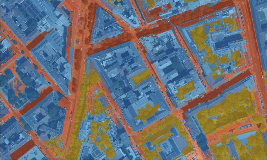
4 IEEE COMMUNICATIONS LETTERS, VOL. 00, NO. 00, MARCH 2020
The obtained reward R, as a result of the action is defined as Algorithm 2 Optimal path search for multi-hop connectivity.
Input: Categorical matrix M.
Rb for transmission across buildings, Output: Optimal Q(s, a) function for multi-hop communication.
Ro for transmission across an open field,
R= Q- LEARNING I TERATION ( IN SECTION II-B.)
(7)
Rs for transmission across a street, 1: Set an arbitrary initial value for Q-table
∞
for reaching the end goal receiver. 2: Let s be the initial state of the matrix environment M
3: for each episode do
For each iteration epoch t, V1 observes the state st and takes 4: Initialize S
an action at , then the state transit into st+1 and V1 receives 5: repeat(for each step of episode)
the reward Rt . The process of observing, selecting an action, 6: Choose at for current st by the -greedy strategy
7: Take action at
and obtaining a reward is repeated and the agent V1 learns Observe the reward Rt+1 , and the
a policy π(st ) ∈ A that maximizes the sum of the rewards
8: new state st+1
Q(st , at ) ← (1 − α)Q(st , at ) + α R + γ max Q(st+1, a)
9:
a
obtained over a time period. In our scenario, maximizing the 10: t ←t+1
sum of the rewards involves minimizing the propagation loss 11: until Q(s, a) converges or reach max. number of iterations.
experienced at the receiver vehicle. To evaluate the value of 12: end for
a state under the policy π, the state-value function can be 13: return Q(s, a) . Optimal state-action function
utilized and is defined as follows.
" ∞ #
π
Õ TABLE I
V (s) = E γ R(st , π(st ))|s0 = s ,
t
(8) S EGMENTATION ACCURACY OBTAINED WITH DIFFERENT M ODELS * .
t=0
Texton Patch Proposed
where γ ∈ [0, 1) represents a discount factor and E[·] is Classes
Forests [5] Based [6]
FCNs [7]
Model**
the expectation operator. To find the optimal policy π ∗ , the
Buildings 47.9% 86.7% 89.4% 92.5%
following Bellman’s optimality criterion can be used. Open Field 45.8% 85.4% 86.5% 90.1%
Streets 40.1% 85.2% 87.4% 89.8%
Õ
V ∗ (s) = max[R(s, a) + γ Ps,a (s 0)V(s 0)], (9)
a∈A * Trainedusing 4 NVIDIA GTX 1080Ti with local parallel pool.
s0
** Convolutional encoder-decoder architecture, optimized with stochastic
where Ps,a (s 0)
is the transition probability from state s to s0 gradient descent with momentum.
when action a is chosen. In this scenario, because Ps,a (s 0)
cannot be easily obtained, Q-learning is considered. For a
policy π, the Q-value corresponding to the state and action using a mini-batch size of 36, an initial learning rate of
pair (s, a) can be defined as, 75 × 10−3 , η of 9 × 10⁻¹ , and L2 regularization factor of
Q π (s, a) = R(s, a) + γ Ps,a (s 0)V π (s 0), 5 × 10⁻⁴ . In our simulations, when β is set to a low value,
Õ
(10)
s0
the training time increases; conversely, when a high value of
β is used, the training duration decreases at the expense of
which is the expected discounted reward of executing action
accuracy. After applying grid search, β = 0.02 is selected. In
a at state s and following policy π thereafter. By setting
Õ our experiments, an end-to-end pixel-wise semantic inference
∗ ∗
Q (s, a) = R(s, a) + γ Ps,a (s 0)V (s 0), (11) is achieved at 65ms per image. The first stage of our model is
s0 compared against well-known segmentation techniques. Our
V ∗ (s) can be replaced by maxa ∈ A Q∗ (s, a). According to [14], proposal increases the average per-class segmentation accu-
racy from 87.76% in FCNs to 90.8% (Table I). The complexity
Q t+1 (s, a) =Q t (s, a) + α(R(s, a))+ of the value-iteration algorithm in the Q-learning problem is
(12)
α γ max Q t (s 0, a 0) − Q t (s, a) .
0
O(en), where e represents the total number of actions, and
a ∈A
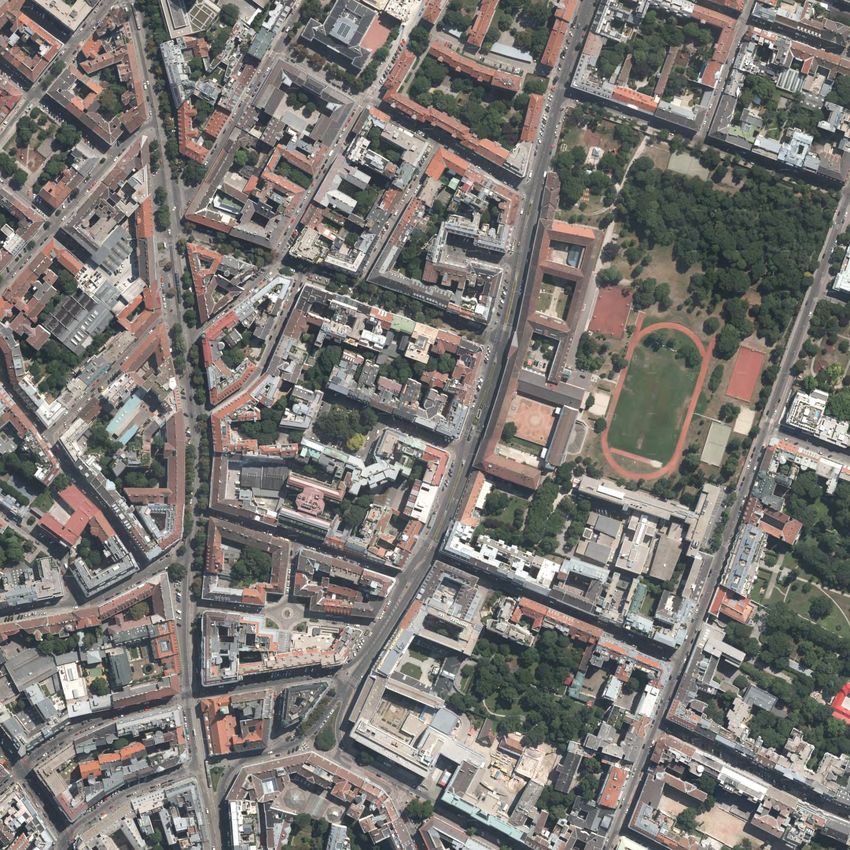
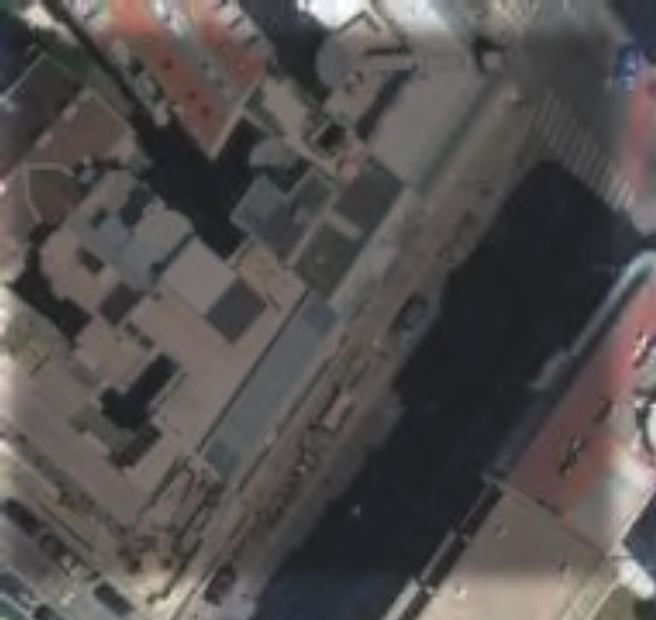
n is the size of the state space [15]. Fig. 2(a) shows an
Here, α is the learning rate. With (12), Q-learning helps the aerial image used for the validation of our model. Fig. 2(b)
agent learn the optimal Q-values recursively by obtaining state presents the semantic image obtained using our upgraded
st and reward Rt and selecting an action at at each time t. architecture. Fig. 2(c) shows the collection of all states s
The iteration will then converge to the optimal value V ∗ and that constitutes the categorical matrix M down-sampled to
policy π ∗ . An -greedy strategy is adopted to decide an action a size of 50×50 pixels. Finally, Fig. 2(d) shows the path
for each iteration. While the agent chooses a random action generated using our transmission policy π ∗ applying the off-
with a probability p to gather more information, it selects the policy model-free algorithm on the categorical matrix M, with
best action given current information with a probability 1 − p. the transmitting vehicle located in the top-left corner, and the
Algorithm 2 provides the pseudo-code of the Q-learning task. receiver in the bottom-right edge of the map. The reward
values employed are Rb = −50, Ro = −10, and Rs = −1. Fig. 3
III. P ERFORMANCE A NALYSIS AND R ESULTS illustrates the central tendency of the received signal strength
The wireless scenario is simulated in MATLAB using an (RSS) at the receiver for both scenarios under study. We find
end-to-end IEEE 802.11p link under a V2X fading channel that with a typical sensitivity of -98dBm at the receiver, the
with additive white Gaussian noise for different distance signal is lost at approximately 300 m when using the shortest-
scales. The network is configured without node signal ampli- distance multi-hop, whereas the proposed lowest-propagation
fication. The convolutional model is trained for 200 epochs, multi-hop strategy does not compromise the range until 500m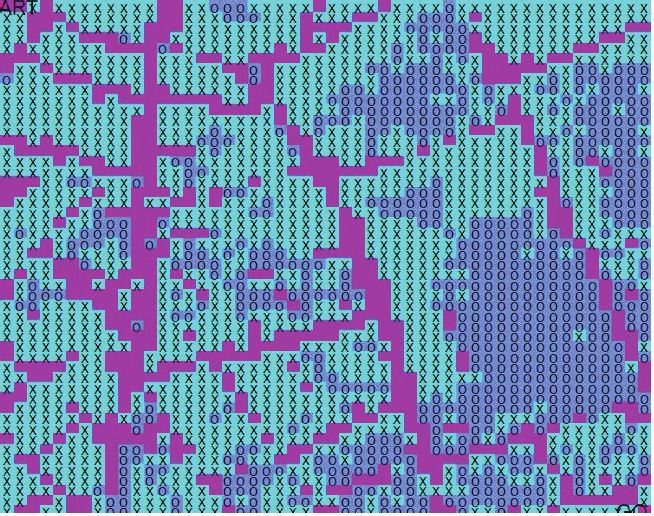
MOROCHO-CAYAMCELA et al.: MACHINE LEARNING TO IMPROVE MULTI-HOP SEARCHING AND EXTENDED WIRELESS REACHABILITY IN V2X 5
TX TX
RX1
Low propagation loss RX2
multihop relay selection.
Shortest-distance
multihop relay selection.
RX RX3
(a) (b) (c) (d)
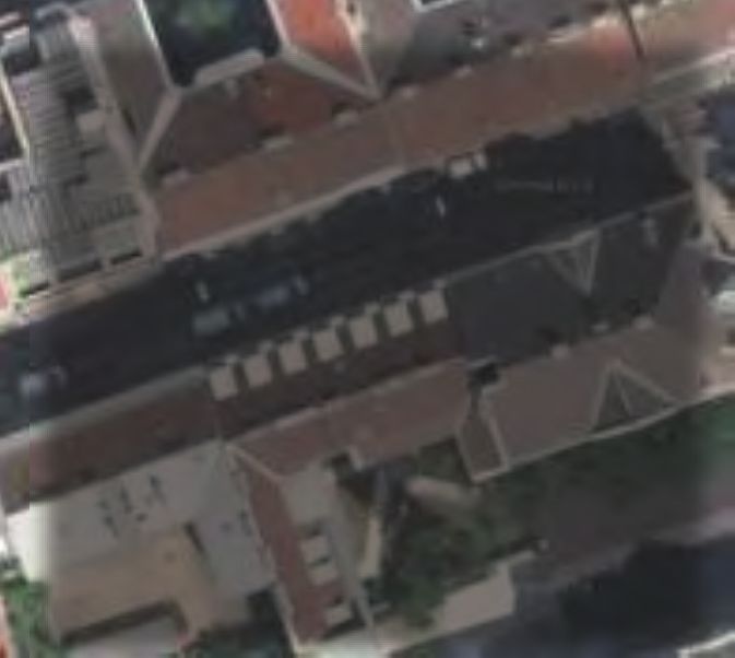
Fig. 2. Simulation results. (a) An aerial image unseen by our model, (b) the pixel-wise segmentation of our enhanced CNN encoder-decoder showing the
buildings on blue, open fields in yellow, and streets in red, (c) the categorical matrix generated from the image segmentation (down-sampled to 50×50 pixels),
(d) paths to three goal receivers generated with the shortest distance strategy [3], and with our multi-hop selection policy that minimizes the propagation loss.
-30
Optimal-path transmission vs. direct-path transmission to surround new obstacles, or discover policies that allows
freq = 5.9GHz transmission across new obstacles to maximize reachability
Received signal strength at the receiver (dBm)
-40 IEEE 802.11p are of interest. Finally, we hope our findings will encourage
sensitivity = -98dBm
-50 researchers to fuse satellite imagery with 3-dimensional maps
of cities (i.e., height of the terrain, buildings, trees, etc), to
-60
enable full machine-learning-driven channel characterization.
-70
R EFERENCES
-80
[1] G. Karagiannis et al., “Vehicular Networking: A Survey and Tutorial
on Requirements, Architectures, Challenges, Standards and Solutions,”
-90
IEEE Commun. Surveys & Tuts., vol. 13, no. 4, pp. 584–616, 2011.
[2] M. Tullsen, L. Pike, N. Collins, and A. Tomb, “Formal Verification
-100
of a Vehicle-to-Vehicle (V2V) Messaging System,” in Computer Aided
-110
Verification. Springer, Cham, 7 2018, pp. 413–429.
Transmission via the optimal path
Transmission via a direct path
[3] I. A. Abbasi et al., “A Reliable Path Selection and Packet Forwarding
-120 Routing Protocol for Vehicular Ad hoc Networks,” EURASIP J. on Wirel.
0 100 200 300 400 500 600 Comms. and Netw., vol. 2018, no. 1, p. 236, 12 2018.
Distance between transmitter and receiver (m) [4] M. E. Morocho-Cayamcela et al., “Machine Learning for 5G/B5G Mo-
bile and Wireless Communications: Potential, Limitations, and Future
Fig. 3. Proposal performance and comparison. With a receiver sensitivity of Directions,” IEEE Access, vol. 7, pp. 137 184–137 206, 9 2019.
-98dbm, the signal is lost around 300m when using a shortest-distance path, [5] J. Shotton, M. Johnson, and R. Cipolla, “Semantic texton forests for
whereas the use of our lowest-propagation loss policy extends the range to image categorization and segmentation,” in 2008 IEEE Conference on
approximately 500m. Our proposal attains a higher RSS at the receiver for Computer Vision and Pattern Recognition. IEEE, 6 2008, pp. 1–8.
all the range of distances when compared with the direct link. [6] D. Ciresan et al., “Deep Neural Networks Segment Neuronal Membranes
in Electron Microscopy Images,” in NIPS Proceedings: Advances in
Neural Info. Processing Systems, 2012, pp. 2843–2851.
[7] E. Shelhamer, J. Long, and T. Darrell, “Fully Convolutional Networks
approximately. These results establish that our system can for Semantic Segmentation,” IEEE Transactions on Pattern Analysis and
extend the coverage of a V2X links by 66.7%. In addition, Machine Intelligence, vol. 39, no. 4, pp. 640–651, 4 2017.
[8] V. Badrinarayanan et al., “Segnet: A deep convolutional encoder-decoder
Fig. 3 reveals that for all distances, the RSS at the receiver is architecture for image segmentation,” IEEE Trans. on Pattern Anal. and
higher when the proposed multi-hop strategy is used. Mach. Intell., vol. 39, no. 12, pp. 2481–2495, 2015.
[9] E. Maggiori et al., “Can Semantic Labeling Methods Generalize to Any
City? The Inria Aerial Image Labeling Benchmark,” 2017 IEEE Int.
IV. C ONCLUSIONS AND F UTURE W ORK Geoscience and Remote Sensing Symp. (IGARSS), pp. 3226–3229, 2017.
[10] ——, “High-Resolution Aerial Image Labeling with Convolutional Neu-
The first stage of our proposal increased the average seg- ral Networks,” IEEE Transactions on Geoscience and Remote Sensing,
mentation accuracy by 44.6%, 5.03%, and 3.04%, compared vol. 55, no. 12, pp. 7092–7103, 12 2017.
with the texton forest, patch-based, and FCN architectures, [11] K. Simonyan and A. Zisserman, “Very Deep Convolutional Networks for
Large-Scale Image Recognition,” International Conference on Learning
respectively. Simulations revealed that our selection policy Representations (ICRL), pp. 1–14, 2015.
improved the multi-hop reachability by 66.7% compared with [12] A. Geron, Hands-On Machine Learning with Scikit-Learn and Tensor-
the shortest-path selection strategy. Our solution could be Flow: Concepts, Tools, and Techniques to build Intelligent Systems,
1st ed., N. Tache, Ed. O’Reilly Media, Inc., 2017.
further studied in device-to-device communications, nomadic [13] R. S. Sutton and A. G. Barto, Reinforcement Learning: An Introduction,
nodes, network routing, path planning, etc. The frequency can 2nd ed. London, England: The MIT Press, 2018.
be modified to 5G and beyond 5G millimeter wave ranges. [14] Junhong Nie and S. Haykin, “A dynamic channel assignment policy
through Q-learning,” IEEE Trans. on Neural Netw., vol. 10, no. 6, pp.
Further work will include enhancing the segmentation model 1443–1455, 1999.
to include more precise categories (i.e., mountains, suburban [15] S. Koenig and R. G. Simmons, “Complexity analysis of real-time
environment, highways, etc.). The prospects of the agent reinforcement learning,” in AAAI Proceedings, 1993, pp. 99–107.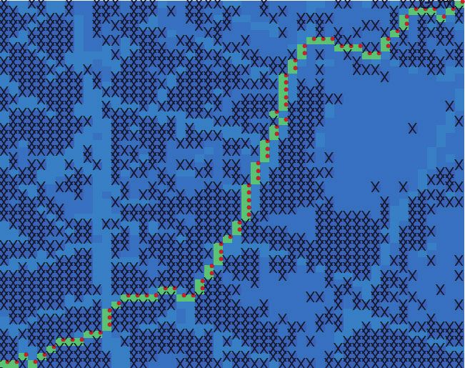


You can also read