Deep Lidar CNN to Understand the Dynamics of Moving Vehicles - UPC
←
→
Page content transcription
If your browser does not render page correctly, please read the page content below
Deep Lidar CNN to Understand the Dynamics of Moving Vehicles
                                  Victor Vaquero, Alberto Sanfeliu, Francesc Moreno-Noguer

   Abstract— Perception technologies in Autonomous Driving
are experiencing their golden age due to the advances in Deep
Learning. Yet, most of these systems rely on the semantically
rich information of RGB images. Deep Learning solutions
applied to the data of other sensors typically mounted on
autonomous cars (e.g. lidars or radars) are not explored much.
In this paper we propose a novel solution to understand the
dynamics of moving vehicles of the scene from only lidar
                                                                                        Pretext tasks - Priors
information. The main challenge of this problem stems from
the fact that we need to disambiguate the proprio-motion of
the “observer” vehicle from that of the external “observed”
vehicles. For this purpose, we devise a CNN architecture which                           Lidar-Flow        Vehicles Mask
at testing time is fed with pairs of consecutive lidar scans.                                   Odometry
However, in order to properly learn the parameters of this
network, during training we introduce a series of so-called               Fig. 1: We present a deep learning approach that, using only
pretext tasks which also leverage on image data. These tasks              lidar information, is able to estimate the ground-plane motion
include semantic information about vehicleness and a novel
                                                                          of the surrounding vehicles. In order to guide the learning
lidar-flow feature which combines standard image-based optical
flow with lidar scans. We obtain very promising results and               process we introduce to our deep framework prior semantic
show that including distilled image information only during               and pixel-wise motion information, obtained from solving
training, allows improving the inference results of the network           simpler pretext tasks, as well as odometry measurements.
at test time, even when image data is no longer used.

                      I. INTRODUCTION
                                                                          to new Convolutional Neural Networks (CNNs) and their
   Capturing and understanding the dynamics of a scene is a
                                                                          ability to capture complex abstract concepts given enough
paramount ingredient for multiple autonomous driving (AD)
                                                                          training samples. However, in an AD environment cameras
applications such as obstacle avoidance, map localization and
                                                                          may suffer a significant performance decrease under abrupt
refinement or vehicle tracking. In order to efficiently and
                                                                          changes of illumination or harsh weather conditions, as for
safely navigate in our unconstrained and highly changing
                                                                          example driving at sunset, night or under heavy rain. On the
urban environments, autonomous vehicles require precise
                                                                          contrary, radar and lidar-based systems performance is robust
information about the semantic and motion characteristics of
                                                                          to these situations. While radars are able to provide motion
the objects in the scene. Special attention should be paid to
                                                                          clues of the scene, their unstructured information and their
moving elements, e.g. vehicles/pedestrians, mainly if their
                                                                          lack of geometry comprehension make it difficult to use them
motion paths are expected to cross the direction of other
                                                                          for other purposes. Instead, lidar sensors provide very rich
objects or the observer.
                                                                          geometrical information of the 3D environment, commonly
   Estimating the dynamics of moving objects in the environ-
                                                                          defined in a well-structured way.
ment requires both from advanced acquisition devices and
                                                                             In this paper we propose a novel approach to detect the
interpretation algorithms. In autonomous vehicle technolo-
                                                                          motion vector of dynamic vehicles over the ground plane by
gies, environment information is captured through several
                                                                          using only lidar information. Detecting independent dynamic
sensors including cameras, radars and/or lidars. On distilling
                                                                          objects reliably from a moving platform (ego vehicle) is an
this data, research over RGB images from cameras has
                                                                          arduous task. The proprio-motion of the vehicle in which
greatly advanced with the recent establishment of deep
                                                                          the lidar sensor is mounted needs to be disambiguated from
learning technologies. Classical perception problems such
                                                                          the actual motion of the other objects in the scene, which
as semantic segmentation, object detection, or optical flow
                                                                          introduces additional difficulties.
prediction [1], [2], [3], have experienced a great boost due
                                                                             We tackle this challenging problem by designing a novel
  The authors are with the Institut de Robòtica i Informàtica In-       Deep Learning framework. Given two consecutive lidar scans
dustrial, CSIC-UPC, Llorens i Artigas 4-6, 08028 Barcelona, Spain.        acquired from a moving vehicle, our approach is able to
{vvaquero,sanfeliu,fmoreno}@iri.upc.edu
   This work has been supported by the Spanish Ministry of Economy        detect the movement of the other vehicles in the scene
and Competitiveness projects HuMoUR (TIN2017-90086-R) and COL-            which have an actual motion with respect to a “ground”
ROBTRANSP (DPI2016-78957-R) and the Spanish State Research Agency         fixed reference frame (see Figure 1). During inference, our
through the Marı́a de Maeztu Seal of Excellence to IRI (MDM-2016-0656).
The authors also thank Nvidia for hardware donation under the GPU grant   network is only fed with lidar data, although for training
program.                                                                  we consider a series of pretext tasks to help with solving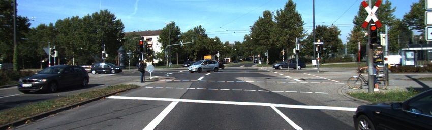
the problem that can potentially exploit image information.           Lidar based approaches to solve the vehicle motion seg-
Specifically, we introduce a novel lidar-flow feature that         mentation problem, have been led by clustering methods,
is learned by combining lidar and standard image-based             either motion- or model-based. The former [12], estimates
optical flow. In addition, we incorporate semantic vehicleness     point motion features by means of RANSAC or similar
information from another network trained on singe lidar            methods, which then are clustered to help on reasoning
scans. Apart from these priors, we introduce knowledge             at object level. Model-based approaches, e.g. [13], initially
about the ego motion by providing odometry measurements            cluster vehicle points and then retrieve those which are
as inputs too. A sketch of our developed approach is shown         moving by matching them through frames.
in Figure 1, where two different scenes are presented along           Although not yet very extended, deep learning techniques
with the corresponding priors obtained from the pretext tasks      are nowadays being also applied to the vehicle detection task
used. The final output shows the predicted motion vectors for      over lidar information. [14] directly applies 3D convolutions
each scene, encoded locally for each vehicle according to the      over the point cloud euclidean space to detect and obtain the
color pattern represented in the ground.                           bounding box of vehicles. As these approaches are compu-
   An ablation study with several combinations of the afore-       tationally very demanding, some authors try to alleviate this
mentioned pretext tasks shows that the use of the lidar-flow       computational burden by sparsifying the convolutions over
feature throws very promising results towards achieving the        the point-cloud [15]. But still the main attitude is to project
overall goal of understanding the motion of dynamic objects        the 3D point cloud into a featured 2D representation and
from lidar data only.                                              therefore being able to apply the well known 2D convolu-
                                                                   tional techniques [16], [13]. In this line of projecting point
                   II. RELATED WORK
                                                                   clouds, other works propose to fuse of RGB images with
   Research on classical perception problems have experi-          lidar front and bird eye features [17].
enced a great boost in recent years, mainly due to the intro-         However, none of these approaches is able to estimate the
duction of deep learning techniques. Algorithms making use         movement of the vehicles in an end-to-end manner without
of Convolutional Neural Networks (CNNs) and variants have          further post-processing the output as we propose. As far
recently matched and even surpassed previous state of the art      as we know, the closer work is [18] which makes use
in computer vision tasks such as image classification, object      of RigidFlow [19] to classify each point as non-movable,
detection, semantic segmentation or optical flow prediction        movable, and dynamic. In this work, we go a step further,
[4], [5], [6], [7].                                                and not only classify the dynamics of the scene, but also
   However, the crucial problem of distinguishing if an object     predict the motion vector of the moving vehicles.
is moving disjointly from the ego motion remains challeng-            Our approach also draws inspiration from progressive
ing. Analysing the motion of the scene through RGB images          neural networks [20] and transfer learning concepts [21]
is also a defiant problem recently tackled with CNNs, with         in that we aim to help the network to solve a complex
several recent articles sharing ideas with our approach. In [8],   problem by solving a set of intermediate “pretext” tasks. For
the authors train a CNN network on synthetic data that taking      instance, in the problem of visual optical flow, [22] and [1]
as input the optical flow between two consecutive images,          use semantic segmentation pretext tasks. Similarly, during
is able to mask independently moving objects. In this paper        training, we also feed the network with prior knowledge
we go a step further and not just distinguish moving objects       about segmented vehicles on the point cloud information.
from static ones, but also estimate their motion vector on
the ground plane reference. Other methods try to disengage
ego and real objects movement by inverting the problem.                 III. D EEP L IDAR - BASED M OTION E STIMATION
For instance, [9] demonstrate that a CNN trained to predict
odometry of the ego vehicle, compares favourably to standard          We next describe the proposed deep learning framework
class-label trained networks on further trained tasks such as      to estimate the actual motion of vehicles in a scene indepen-
scene and object recognition. This fact suggests that it is        dently from the ego movement, and using only lidar informa-
possible to exploit ego odometry knowledge to guide a CNN          tion. Our approach relies on a Fully Convolutional Network
on the task of disambiguating our movement from the free           that receives as input featured lidar information from two
scene motion, which we do in Section III-B.                        different but temporary close frames of the scene, and outputs
   The aforementioned works, though, are not focused on AD         a dense estimation of the ground-floor motion vector of each
applications. On this setting, common approaches segment           point, given the case that it belongs to a dynamic vehicle.
object motion by minimizing geometrically-grounded energy          For that, in Section III-A we introduce a novel dataset built
functions. [10] assumes that outdoor scenes can decompose          from the Kitti tracking benchmark that has been specifically
into a small number of independent rigid motions and jointly       created to be used as ground-truth in our supervised problem.
estimate them by optimizing a discrete-continuous CRF. [11]        Since lidar information by itself is not enough to solve the
estimates the 3D dynamic points in the scene through a             proposed complex mission, in Section III-B we consider
vanishing point analysis of 2D optical-flow vectors. Then, a       exploiting pretext tasks to introduce prior knowledge about
three-term energy function is minimized in order to segment        the semantics and the dynamics of the scene to the main
the scene into different motions.                                  CNN defined in Section III-C.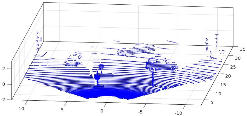
Ranges

                                                        Reflectivity
                                  Network Inputs

  (a) Basic point cloud frame input data. Ranges and reflectivity      (b) Network output: lidar-based vehicle motion representation.
Fig. 2: Basic input and predicted output. (a) The input of the network corresponds to a pair of lidar scans, which are
represented in 2D domains of range and reflectivity. (b) The output we seek to learn represents the motion vectors of the
moving vehicles, colored here with the shown pattern attending to the motion angle and magnitude.

A. Lidar Motion Dataset                                                ego-odometry measurements. Then, the transformed position
   In order to train a CNN in a supervised manner, we need             of the vehicle centroid is simply:
to define both the input information and the ground-truth                              Ot
                                                                                            Ct+n = (Ot Ttt+n )−1 ·     Ot+n
                                                                                                                                Ct+n   (1)
of the desired output from which to compare the learned
estimations.                                                           and the on-ground motion vector of the free moving vehicle
   The simpler input data we use consists on the concatena-            in the analysed interval can be calculated as Ot Ct+n − Ot Ct .
tion of two different projected lidar scans featuring the ranges          Notice that these ground-truth needs to be calculated in a
and reflectivity measured, as the one shown in Figure 2a. For          temporal sliding window manner using the lidar scans from
each scan, we transform the corresponding points of the point          frames t and t + n and therefore, different results will be
cloud from its 3D euclidean coordinates to spherical ones,             obtained depending on the time step n. The bigger this time
and project those to a 2D domain attending to the elevation            step is, the longer will be the motion vector, but it will be
and azimuth angles. Each row corresponds to one of the                 harder to obtain matches between vehicles.
sensor vertical lasers (64) and each column is equivalent                 Some drift is introduced as accumulation of errors from
to a laser step in the horizontal field of view (448). This            i) the Kitti manual annotation of bounding boxes, ii) noise
field of view is defined attending to the area for which the           in the odometry measurements and iii) the transformations
Kitti dataset provides bounding box annotations, that covers           numerical resolution. This made that some static vehicles
approximately a range of [−40.5, 40.5] degrees from the ego            were tagged as slightly moving. We therefore filtered the
point of view. Each pair (u, v) of the resulting projection            moving vehicles setting as dynamic only the ones which
encodes the sensor measured range and reflectivity. A more             displacement is larger than a threshold depending on the
detailed description of this process can be found in [13].             time interval n, and consequently, directly related to the
   To build the desired ground-truth output, we make use               minimum velocity from which we consider a movement. We
of the annotated 3D bounding boxes of the Kitti Tracking               experimentally set this threshold to 10Km/h.
Benchmark dataset [2], that provides diversity of motion                  Finally, we encode each vehicle ground-truth motion vec-
samples. As nowadays vehicles still move on the ground                 tor attending to its angle and magnitude according to the
plane, we stated its motion as a two - dimensional vector over         color-code typically used to represent optical flow. Figure 2b
the Z/X plane, being Z our forward ego direction and X its             shows a frame sample of the described dataset, where the
transversal one. For each time t, we define our ego-vehicle            corresponding RGB image of the scene is also shown just
position as Ot ∈ R2 , i.e the observer. Considering there are          for comparison purposes. 1 .
X vehicle tracks in the scene at each moment, we define
any of these vehicle centroids as seen from the observer               B. Pretext tasks
frame of reference like Ot Ct,x ∈ R2 where x = 1 . . . X .                As aforementioned, we guide the network learning towards
For a clearer notation, we will show a use case with just              the correct solution introducing prior knowledge obtained by
one free moving vehicle, omitting therefore the x index. As            solving other pretext tasks. This idea draws similarities from
both the observer and the other vehicle are moving, we will            progressive networks [20] and transfer learning works [9],
see the free vehicle centroid Ot+n Ct+n each time from a               both helping in solving increasing complexity tasks. In this
different position Ot+n . Therefore, in order to get the real          manner, we introduce three kinds of additional information:
displacement of the object in the interval t → t + n we need           a) a lidar-optical flow motion prior to guide our network for
to transform this last measurement to our previous reference           finding matches between the two lidar inputs; b) semantic
frame Ot , obtaining Ot Ct+n . Let us denote our own frame
displacement as Ot Ttt+n , which is known by the differential            1 We   plan to make our datasets publicly available.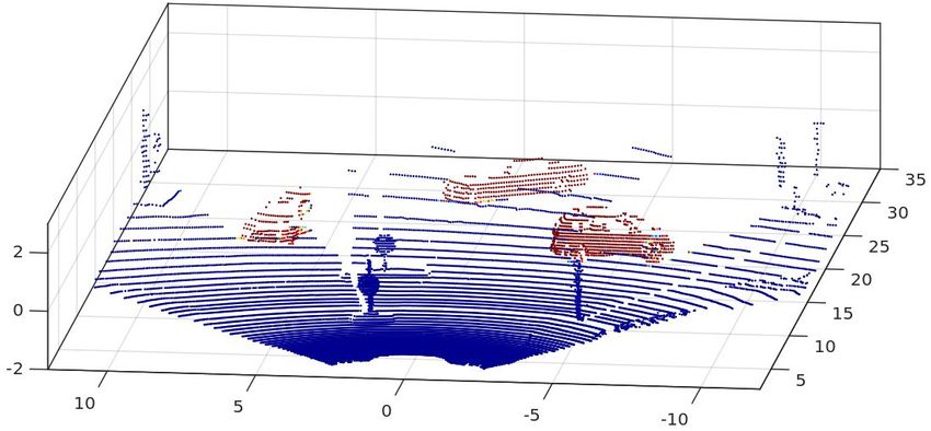
Ranges

                                                                                                                     “Vehicleness” Prior
                                                                        Reflectivity

                                                                                                 CNN

                           GT generation

                                               Lidar-Flow Prediction
                                                                       Point Cloud                                Predicted Point Cloud

                      (a) Lidar-flow prior                                                   (b) Semantic prior
Fig. 3: Pretext tasks used to guide the final learning. a) lidar-flow prior, obtained by processing pairs of frames through a
new learned lidar-flow net; b) semantic prior, obtained by processing single frames through our vehicle lidar-detector net.

concepts that will help with focusing on the vehicles in                  We first transformed the network expansive part by in-
the scene; c) the ego motion information based on the                  troducing new deconvolutional blocks at the end with the
displacement given by the odometry measurements.                       respective batch normalization (BN) and non-linearity im-
   The motion prior for matching inputs is given by stating            position (Relu). Standard FlowNet output is sized a fourth
a novel deep-flow feature map that can be seen in Figure 3a.           of the input and bi-linearly interpolated in a subsequent
We developed a new deep framework that takes as input the              step. This is not applicable to our approach as our desired
2D projection of lidar scans from two separated frames and             output is already very sparse containing only few groups
outputs a learned lidar-based optical flow. As lidar-domain            of lidar points that belong to moving vehicles. Therefore
optical flow ground-truth is not available, we created our             mid resolution outputs may not account for far vehicles that
own for this task. To do this, we used a recent optical                are detected by only small sets of points. In addition, we
flow estimator [7] based on RGB images and obtained flow               eliminate both the last convolution and first deconvolution
predictions for the full Kitti tracking dataset. We further            blocks of the inner part of FlowNet, for which the generated
created a geometric model of the given lidar sensor attending          feature maps reach a resolution of 1/64 over the initial
to the manufacturer specifications and projected it over the           input size. Note that our lidar input data has per se low
predicted flow maps, obtaining the corresponding lidar-flow            resolution (64 × 448), and performing such an aggressive
of each point in the point cloud. Finally we stated a dense            resolution reduction has been shown to result in missing
deep regression problem that uses the new lidar-flow features          targets. On the other hand, we follow other FlowNet original
as ground-truth to learn similar 2D motion patterns using a            attributes. Thus, our architecture performs a concatenation
flownet-alike convolutional neural network.                            between equally sized feature maps from the contractive and
   Semantic priors about the vehicleness of the scene are              the expansive parts of the network which produce richer
introduced via solving a per-pixel classification problem like         representations and allows better gradient flow. In addition,
the one presented in [13]. For it, a fully convolutional net-          we also impose intermediate loss optimization points obtain-
work is trained to take a lidar scan frame and classifies each         ing results at different resolutions which are upsampled and
corresponding point as belonging to a vehicle or background.           concatenated to the immediate upper feature maps, guiding
An example of these predictions is shown in Figure 3b.                 the final solution from early steps and allowing the back-
   Finally, we introduce further information about the ego-            propagation of stronger and healthier gradients.
motion in the interval. For this, we create a 3 channel matrix
with the same size as the 2D lidar feature maps where                                        IV. E XPERIMENTS
each “pixel” triplet takes the values for the forward (Z) and            This section provides a thorough analysis of the perfor-
transversal (X) ego-displacement as well as the rotation over          mance of our framework fulfilling the task of estimating the
Y axis in the interval t → t + n.                                      motion vector of moving vehicles given two lidar scans.

C. Deep-Lidar Motion Network                                           A. Training details
   As network architecture for estimating the rigid motion                For training the presented deep neural networks from both
of each vehicle over the ground floor, we considered the               the main framework and the pretext tasks, we set n to 1,
Fully Convolutional Network detailed in Figure 4. It draws             so that measuring the vehicles movement between two time
inspiration from FlowNet [23], which is designed to solve              consecutive frames. All these networks are trained from zero,
a similar regression problem. However, we introduced some              initializing them with the He’s method [24] and using Adam
changes to further exploit the geometrical nature of our lidar         optimization with the standard parameters β1 = 0.9 and
information.                                                           β2 = 0.999.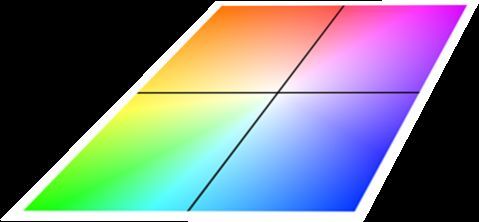
64 2         128 2     256 2          256 1             512 2       512 1        1024 2       1024 1
                                        7   *3        5   *2    5   *2             3   *1        3   *1         3   *1     3   *1         3   *1
                                                                                                                                                   M S Convolution
                                                                                                                                                     *
                                                                                                                                                   N P M (out channels) S (stride),
                                                                                                                                                          NxN (filter size)   P (padding)

                                                     512                     512                          512                       512                   Batch Normalization

                                                                                                                                                       M Deconvolution Up x2

                                    *
                                                                                                                                                          M (out channels)
                                                                                                                                                          4x4 (filter size), Crop 1
                                                                                                                                                   *      Intermediate Prediction
     Veh. Motion Predictions                                                                                                                              1x1 conv, s = 1, p = 0 Up x2

                                                 *

                                                                         *

                                                                                                      *

                                                                                                                                *
                                                                                                                                                          Leaky ReLu (10%)

                                                                                                                                                          Loss Calculation

                     Ground-Truth

      Fig. 4: Deep Learning architecture used to predict the motion vector of moving vehicles from two lidar scans.

   The Kitti Tracking benchmark contains a large number of                                  indicate the predicted probability of each pixel to belong to
frames with static vehicles, which results in a reduction of the                            a vehicle. This information is further concatenated with the
number of samples from which we can learn. Our distilled                                    raw lidar input plus the lidar-flow maps, yielding a tensor
Kitti Lidar-Motion dataset contains 4953 frames with moving                                 with a depth of 8 channels.
vehicles, and 3047 that either contain static vehicles or do                                   Finally, for introducing the odometry information as well,
not contain any. To balance the batch sampling and avoid a                                  three more channels are concatenated to the stacked input
biased learning, we take for each batch 8 frames containing                                 resulting in a tensor of depth 11.
movement and 2 that do not. For training all models we
left for validation the sequences 1, 2 and 3 of our distilled                               C. Results
Kitti Training dataset, which results in 472 samples with                                      Table I shows a quantitative analysis of our approach. We
motion and 354 without. As our training samples represent                                   demonstrate the correct performance of our framework by
driving scenes, we perform data augmentation providing only                                 setting two different baselines, error@zero and error@mean.
horizontal flips with a 50% chance, in order to preserve the                                The first one assumes a zero regression, so that sets all the
strong geometric lidar properties.                                                          predictions to zero as if there were no detector. The second
   The training process is performed on a single NVIDIA                                     baseline measures the end-point-error that a mean-motion
1080 Ti GPU for 400, 000 iterations with a batch size of 10                                 output would obtain.
Velodyne scan pairs per iteration. The learning rate is fixed                                  Notice that in our dataset only a few lidar points fall into
to 10−3 during the first 150, 000 iterations, after which, it is                            moving vehicles on each frame. Therefore, measuring the
halved each 60, 000 iterations. As loss, we use the euclidean                               predicted error over the full image does not give us a notion
distance between the ground-truth and the estimated motion                                  about the accuracy of the prediction, as errors generated by
vectors for each pixel. We set all the intermediate calculated                              false negatively (i.e. that are dynamic but considered as static
losses to equally contribute for the learning purposes.                                     without assigning them a motion vector) and false positively
                                                                                            (i.e. that are static but considered as dynamic assigning
B. Input data management for prior information                                              them a motion vector) detected vehicles, would get diluted
   Depending on the data and pretext information introduced                                 over the full image. In order to account for this fact, we
in our main network, different models have been trained;                                    also measure end-point error over the real dynamic points
following, we provide a brief description.                                                  only. Both measurements are indicated in Table I as full and
   Our basic approach takes as input a tensor of size 64 ×                                  dynamic. All the given values are calculated at test time over
448 × 4 which stacks the 2D lidar projected frames from                                     the validation set only, which during the learning phase has
instants t and t + 1. Each projected frame contains values of                               never been used for training neither the main network nor the
the ranges and reflectivity measurements, as summarized at                                  pretext tasks. Recall that during testing, the final networks
the beginning of Section III-A and shown in Figure 2a.                                      are evaluated only using lidar Data.
   For obtaining motion priors, the lidar data is processed                                    We tagged the previously described combinations of inputs
through our specific lidar-flow network. It produces, as out-                               data with D, F , S and O respectively for models us-
put, a two channel flow map where each pair (u,v) represents                                ing Data, Lidar-Flow, Vehicle Segmentation and Odometry.
the RGB equivalent motion vector on the virtual camera                                      When combining different inputs, we express it with the &
alike plane as shown in Figure 3a. When incorporating this                                  symbol between names; e.g. a model named D & F & S
motion prior to the main network, the lidar-flow map is                                     has been trained using as input the lidar Data, plus the priors
concatenated with the basic lidar input to build a new input                                Lidar-Flow and Vehicle Segmentation.
tensor containing 6 depth channels.                                                            At the light of the results several conclusions can be
   In order to add semantic prior knowledge in the training,                                extracted. First, is that only lidar information is not enough
we separately process both lidar input frames through our                                   for solving the problem of estimating the motion vector of
learned vehicle detection network [13]. The obtained outputs                                freely moving vehicles in the ground, as we can see how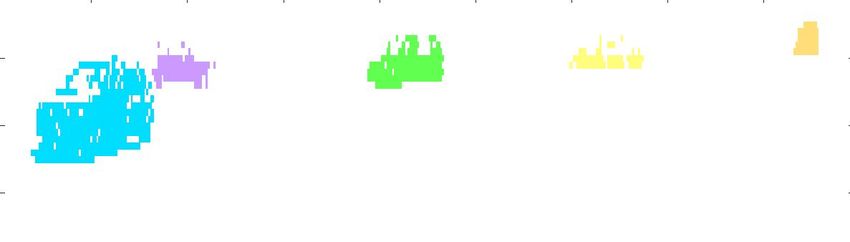
TABLE I: Evaluation results after training the network using
several combination of lidar- and image-based priors. Test is                [3] A. Behl, O. H. Jafari, S. K. Mustikovela, H. A. Alhaija, C. Rother,
                                                                                 and A. Geiger, “Bounding boxes, segmentations and object coordi-
performed using only lidar inputs. Errors are measured in                        nates: How important is recognition for 3d scene flow estimation in
pixels, end-point-error.                                                         autonomous driving scenarios,” in IEEE International Conference on
                                                                                 Computer Vision (ICCV), 2017.
                                         full    dynamic                     [4] K. He, X. Zhang, S. Ren, and J. Sun, “Deep residual learning for image
              error@zero               0.0287     1.3365                         recognition,” in IEEE Conference on Computer Vision and Pattern
              error@mean               0.4486     1.5459                         Recognition (CVPR), 2016.
              D                        0.0369     1.2181                     [5] S. Ren, K. He, R. Girshick, and J. Sun, “Faster r-cnn: Towards real-
              GT.F                     0.0330     1.0558                         time object detection with region proposal networks,” in Advances in
              GT.F & D & S             0.0234     0.8282                         Neural Information Processing Systems (NIPS), 2015.
              Pred.F                   0.0352     1.1570                     [6] J. Long, E. Shelhamer, and T. Darrell, “Fully convolutional networks
              Pred.F & D               0.0326     1.1736                         for semantic segmentation,” in IEEE Conference on Computer Vision
              Pred.F & D & S           0.0302     1.0360                         and Pattern Recognition (CVPR), 2015.
              Pred.F & D & S & O       0.0276     0.9951
                                                                             [7] E. Ilg, N. Mayer, T. Saikia, M. Keuper, A. Dosovitskiy, and T. Brox,
                                                                                 “Flownet 2.0: Evolution of optical flow estimation with deep net-
                                                                                 works,” in IEEE Conference on Computer Vision and Pattern Recog-
the measured dynamic error is close to the error at zero.                        nition (CVPR), 2017.
                                                                             [8] P. Tokmakov, K. Alahari, and C. Schmid, “Learning motion patterns
To account for the strength of introducing optical flow as                       in videos,” in IEEE Conference on Computer Vision and Pattern
motion knowledge for the network, we tested training with                        Recognition (CVPR), 2017.
only the lidar-flow ground truth (GT.F rows in the table) as                 [9] P. Agrawal, J. Carreira, and J. Malik, “Learning to see by moving,”
well as with a combination of flow ground-truth, semantics                       in IEEE International Conference on Computer Vision (ICCV), 2015.
                                                                            [10] M. Menze and A. Geiger, “Object scene flow for autonomous vehi-
and lidar data. Both experiments show favourable results,                        cles,” in IEEE Conference on Computer Vision and Pattern Recogni-
being the second one the most remarkable. However, the                           tion (CVPR), 2015.
lidar-flow ground-truth is obtained from the optical flow                   [11] J.-Y. Kao, D. Tian, H. Mansour, A. Vetro, and A. Ortega, “Moving
extracted using RGB images, which does not accomplish our                        object segmentation using depth and optical flow in car driving
                                                                                 sequences,” in IEEE International Conference on Image Processing
solo-lidar goal. We therefore perform the rest of experiments                    (ICIP), 2016.
with the learned lidar-flow (Pred.F rows in the table) as prior,            [12] A. Dewan, T. Caselitz, G. D. Tipaldi, and W. Burgard, “Motion-based
eliminating any dependence on camera images. As expected,                        detection and tracking in 3d lidar scans,” in IEEE/RSJ International
                                                                                 Conference on Robotics and Automation (ICRA), 2016.
our learned lidar-flow introduce further noise but still allow
                                                                            [13] V. Vaquero, I. del Pino, F. Moreno-Noguer, J. Sola, A. Sanfeliu,
us to get better results than using only lidar information,                      and J. Andrade-Cetto, “Deconvolutional networks for point-cloud
which suggest that flow notion is quite important in order to                    vehicle detection and tracking in driving scenarios,” in IEEE European
solve the major task.                                                            Conference on Mobile Robots (ECMR), 2017.
                                                                            [14] B. Li, “3d fully convolutional network for vehicle detection in point
                        V. C ONCLUSIONS                                          cloud,” in IEEE/RSJ International Conference on Intelligent Robots
                                                                                 and Systems (IROS), 2017.
   In this paper we have addressed the problem of under-                    [15] M. Engelcke, D. Rao, D. Z. Wang, C. H. Tong, and I. Posner,
standing the dynamics of moving vehicles from lidar data                         “Vote3deep: Fast object detection in 3d point clouds using efficient
                                                                                 convolutional neural networks,” in IEEE International Conference on
acquired by a vehicle which is also moving. Disambiguating                       Robotics and Automation (ICRA), 2017.
proprio-motion from other vehicles’ motion poses a very                     [16] B. Li, T. Zhang, and T. Xia, “Vehicle detection from 3d lidar using
challenging problem, which we have tackled using Deep                            fully convolutional network,” in Robotics: Science and Systems (RSS),
Learning. The main contribution of the paper has been to                         2016.
                                                                            [17] X. Chen, H. Ma, J. Wan, B. Li, and T. Xia, “Multi-view 3d object
show that while during testing, the proposed Deep Neural                         detection network for autonomous driving,” in IEEE Conference on
Network is only fed with lidar-scans, its performance can be                     Computer Vision and Pattern Recognition (CVPR), 2017.
boosted by exploiting other prior image information during                  [18] A. Dewan, G. L. Oliveira, and W. Burgard, “Deep semantic classifi-
training. We have introduced a series of pretext tasks for this                  cation for 3d lidar data,” IEEE/RSJ Conference on Intelligent Robots
                                                                                 and Systems (IROS), 2017.
purpose, including semantics about the vehicleness and an                   [19] A. Dewan, T. Caselitz, G. D. Tipaldi, and W. Burgard, “Rigid scene
optical flow texture built from both image and lidar data. The                   flow for 3d lidar scans,” in IEEE/RSJ International Conference on
results we have reported are very promising and demonstrate                      Intelligent Robots and Systems (IROS), 2016.
that exploiting image information only during training really               [20] A. A. Rusu, N. C. Rabinowitz, G. Desjardins, H. Soyer, J. Kirkpatrick,
                                                                                 K. Kavukcuoglu, R. Pascanu, and R. Hadsell, “Progressive neural
helps the lidar-based deep architecture. In future work, we                      networks,” arXiv preprint arXiv:1606.04671, 2016.
plan to further exploit this fact by introducing other image-               [21] J. Yosinski, J. Clune, Y. Bengio, and H. Lipson, “How transferable are
based priors during training, such as the semantic informa-                      features in deep neural networks?,” in Advances in Neural Information
                                                                                 Processing Systems (NIPS), 2014.
tion of all object categories in the scene and dense depth
                                                                            [22] L. Sevilla-Lara, D. Sun, V. Jampani, and M. J. Black, “Optical flow
obtained from images.                                                            with semantic segmentation and localized layers,” in IEEE Conference
                                                                                 on Computer Vision and Pattern Recognition (CVPR), 2016.
                            R EFERENCES                                     [23] A. Dosovitskiy, P. Fischer, E. Ilg, P. Hausser, C. Hazirbas, V. Golkov,
 [1] M. Bai, W. Luo, K. Kundu, and R. Urtasun, “Exploiting semantic              P. van der Smagt, D. Cremers, and T. Brox, “Flownet: Learning optical
     information and deep matching for optical flow,” in European Confer-        flow with convolutional networks,” in IEEE International Conference
     ence on Computer Vision (ECCV), Springer, 2016.                             on Computer Vision (ICCV), 2015.
 [2] A. Geiger, P. Lenz, and R. Urtasun, “Are we ready for autonomous       [24] K. He, X. Zhang, S. Ren, and J. Sun, “Delving deep into rectifiers:
     driving? the kitti vision benchmark suite,” in IEEE Conference on           Surpassing human-level performance on imagenet classification,” in
     Computer Vision and Pattern Recognition (CVPR), 2012.                       IEEE International Conference on Computer Vision (ICCV), 2015.
You can also read