Camera-Based Navigation of a Low-Cost Quadrocopter
←
→
Page content transcription
If your browser does not render page correctly, please read the page content below
Camera-Based Navigation of a Low-Cost Quadrocopter
                                        Jakob Engel, Jürgen Sturm, Daniel Cremers

   Abstract— In this paper, we describe a system that enables
a low-cost quadrocopter coupled with a ground-based laptop
to navigate autonomously in previously unknown and GPS-
denied environments. Our system consists of three components:
a monocular SLAM system, an extended Kalman filter for
data fusion and state estimation and a PID controller to
generate steering commands. Next to a working system, the
main contribution of this paper is a novel, closed-form solution
to estimate the absolute scale of the generated visual map
from inertial and altitude measurements. In an extensive set of
experiments, we demonstrate that our system is able to navigate
in previously unknown environments at absolute scale without
requiring artificial markers or external sensors. Furthermore,
we show (1) its robustness to temporary loss of visual tracking    Fig. 1. A low-cost quadcopter navigates in unstructured environments
and significant delays in the communication process, (2) the       using the front camera as its main sensor. The quadrocopter is able to hold a
elimination of odometry drift as a result of the visual SLAM       position, fly figures with absolute scale, and recover from temporary tracking
system and (3) accurate, scale-aware pose estimation and           loss. Picture taken at the TUM open day.
navigation.

                     I. I NTRODUCTION                                 The motivation behind our work is to showcase that robust,
                                                                   scale-aware visual navigation is feasible and safe on low-cost
   In recent years, research interest in autonomous micro-         robotic hardware. As a platform, we use the Parrot AR.Drone
aerial vehicles (MAVs) has grown rapidly. Significant              which is available for $300 and, with a weight of only 420 g
progress has been made, recent examples include aggressive         and a protective hull, safe to be used in public places (see
flight maneuvers [1, 2], ping-pong [3] and collaborative           Fig. 1). As the onboard computational resources are utterly
construction tasks [4]. However, all of these systems require      limited, all computations are performed externally.
external motion capture systems. Flying in unknown, GPS-
                                                                      The contribution of this paper is two-fold: first, we derive
denied environments is still an open research problem. The
                                                                   a maximum-likelihood estimator to determine the map scale
key challenges here are to localize the robot purely from its
                                                                   in closed-form from metric distance measurements. Second,
own sensor data and to robustly navigate it even under poten-
                                                                   we provide a robust technique to deal with large delays in
tial sensor loss. This requires both a solution to the so-called
                                                                   the controlled system, which facilitates the use of a ground
simultaneous localization and mapping (SLAM) problem as
                                                                   station in the control loop. Two videos demonstrating the
well as robust state estimation and control methods. These
                                                                   robustness of our approach, its ability to eliminate drift
challenges are even more expressed on low-cost hardware
                                                                   effectively and to estimate the absolute scale of the map are
with inaccurate actuators, noisy sensors, significant delays
                                                                   available online:
and limited onboard computation resources.
   For solving the SLAM problem on MAVs, different types                        http://youtu.be/tZxlDly7lno
of sensors such laser range scanners [5], monocular cameras                     http://youtu.be/eznMokFQmpc
[6, 7], stereo cameras [8] and RGB-D sensors [9] have been
explored in the past. In our point of view, monocular cameras
                                                                                            II. R ELATED W ORK
provide two major advantages above other modalities: (1)
the amount of information that can be acquired is immense             Previous work on autonomous flight with quadrocopters
compared to their low weight, power consumption, size and          can be categorized into different research areas. One part of
cost, which are unmatched by any other type of sensor              the community focuses on accurate quadrocopter control and
and (2) in contrast to depth measuring devices, the range          a number of impressive results have been published [10, 1,
of a monocular camera is virtually unlimited – allowing a          3]. These works however rely on advanced external tracking
monocular SLAM system to operate both in small, confined           systems, restricting their use to a lab environment. A similar
and large, open environments. The drawback however is,             approach is to distribute artificial markers in the environment,
that the scale of the environment cannot be determined from        simplifying pose estimation [11]. Other approaches learn a
monocular vision alone, such that additional sensors (such         map offline from a previously recorded, manual flight and
as an IMU) are required.                                           thereby enable a quadrocopter to again fly the same trajectory
                                                                   [12]. For outdoor flights where GPS-based pose estimation
  J. Engel, J. Sturm and D. Cremers are with the Department
of Computer Science, Technical University of Munich, Germany       is possible, complete solutions are available as commercial
{engelj,sturmju,cremers}@in.tum.de                                 products [13].
In this work we focus on autonomous flight without previ-
ous knowledge about the environment nor GPS signals, while
using only onboard sensors. First results towards this goal
have been presented using a lightweight laser scanner [5], a
Kinect [9] or a stereo rig [8] mounted on a quadrocopter as
primary sensor. While these sensors provide absolute scale
of the environment, their drawback is a limited range and                      video @ 18 Hz           IMU @ 200 Hz            control
                                                                               320 × 240               altimeter @ 25 Hz       @ 100 Hz
large weight, size and power consumption when compared
to a monocular setup [14, 7].                                       wireless
   In our work we therefore focus on a monocular camera for          LAN                                                       ∼ 60 ms
                                                                               ∼ 130 ms delay          ∼ 30-80 ms delay
pose estimation. Stabilizing controllers based on optical flow                                                                 delay
were presented in [15], and similar methods are integrated
in commercially available hardware [16]. Such systems how-
ever are subject to drift over time, and hence not suited for            monocular               extended                   PID
                                                                          SLAM                  Kalman filter              control
long-term navigation.
   To eliminate drift, various monocular SLAM methods
have been investigated on quadrocopters, both with off-board       Fig. 2. Approach Outline: Our navigation system consists of three major
                                                                   components: a monocular SLAM implementation for visual tracking, an
[14, 5] and on-board processing [7]. A particular challenge        EKF for data fusion and prediction, and PID control for pose stabilization
for monocular SLAM is, that the scale of the map needs             and navigation. All computations are performed offboard, which leads to
to be estimated from additional metric sensors such as IMU         significant, varying delays which our approach has to compensate.
or GPS, as it cannot be recovered from vision alone. This
problem has been addressed in recent publications such as          A. Sensors
[17, 18]. The current state of the art is to estimate the scale       The AR.Drone is equipped with a 3-axis gyroscope and
using an extended Kalman filter (EKF), which contains scale        accelerometer, an ultrasound altimeter and two cameras. The
and offset in its state. In contrast to this, we propose a novel   first camera is aimed forward, covers a field of view of
approach which is based on direct computation: Using a             73.5◦ × 58.5◦ , has a resolution of 320 × 240 and a rolling
statistical formulation, we derive a closed-form, consistent       shutter with a delay of 40 ms between the first and the last
estimator for the scale of the visual map. Our method              line captured. The video of the first camera is streamed to a
yields accurate results both in simulation and practice, and       laptop at 18 fps, using lossy compression. The second camera
requires less computational resources than filtering. It can       aims downward, covers a field of view of 47.5◦ × 36.5◦ and
be used with any monocular SLAM algorithm and sensors              has a resolution of 176 × 144 at 60 fps. The onboard software
providing metric position or velocity measurements, such           uses the down-looking camera to estimate the horizontal
as an ultrasonic or pressure altimeter or occasional GPS           velocity. The quadcopter sends gyroscope measurements and
measurements.                                                      the estimated horizontal velocity at 200 Hz, the ultrasound
   In contrast to the systems presented in [14, 7], we deliber-    measurements at 25 Hz to the laptop. The raw accelerometer
ately refrain from using expensive, customized hardware: the       data cannot be accessed directly.
only hardware required is the AR.Drone, which comes at a
costs of merely $300 – a fraction of the cost of quadrocopters     B. Control
used in previous work. Released in 2010 and marketed as               The onboard software uses these sensors to control the roll
high-tech toy, it has been used and discussed in several           Φ and pitch Θ, the yaw rotational speed Ψ̇ and the vertical
research projects [19, 20, 21]. To our knowledge, we are the       velocity ż of the quadrocopter according to an external
first to present a complete implementation of autonomous,          reference value. This reference is set by sending a new
camera-based flight in unknown, unstructured environments                                             ¯ ) ∈ [−1, 1]4 every 10 ms.
                                                                   control command u = (Φ̄, Θ̄, ż¯, Ψ̇
using the AR.Drone.
                                                                                              IV. A PPROACH
                III. H ARDWARE P LATFORM                              Our approach consists of three major components running
  As platform we use the Parrot AR.Drone, a commercially           on a laptop connected to the quadrocopter via wireless LAN,
available quadrocopter. Compared to other modern MAV’s             an overview is given in Fig. 2.
such as Ascending Technology’s Pelican or Hummingbird                 1) Monocular SLAM: For monocular SLAM, our solu-
quadrocopters, its main advantage is the very low price, its       tion is based on Parallel Tracking and Mapping (PTAM) [22].
robustness to crashes and the fact that it can safely be used      After map initialization, we rotate the visual map such that
indoor and close to people. This however comes at the price        the xy-plane corresponds to the horizontal plane according
of flexibility: Neither the hardware itself nor the software       to the accelerometer data, and scale it such that the average
running onboard can easily be modified, and communication          keypoint depth is 1. Throughout tracking, the scale of the
with the quadrocopter is only possible over wireless LAN.          map λ ∈ R is estimated using a novel method described in
With battery and hull, the AR.Drone measures 53 cm×52 cm           Section IV-A. Furthermore, we use the pose estimates from
and weights 420 g.                                                 the EKF to identify and reject falsely tracked frames.
∼ 100 ms    ∼ 25 ms     ∼ 125 ms                 ties from additional, metric sensors such as an ultrasound
  vis. pose:                                                                    altimeter.
      ẋ, ẏ, z:                                                                   As a first step, the quadrocopter measures in regular
   Φ, Θ, Ψ:                                                                     intervals the d-dimensional distance traveled both using only
 prediction:                                                                    the visual SLAM system (subtracting start and end position)
                                                                                and using only the metric sensors available (subtracting start
                   t − ∆tvis                               t    t + ∆tcontrol
                                                                                and end position, or integrating over estimated speeds). Each
Fig. 3.    Pose Prediction: Measurements and control commands arrive            interval gives a pair of samples xi , yi ∈ Rd , where xi is scaled
with significant delays. To compensate for these delays, we keep a history
of observations and sent control commands between t −∆tvis and t +∆tcontrol     according to the visual map and yi is in metric units. As both
and re-calculate the EKF state when required. Note the large timespan with      xi and yi measure the motion of the quadrocopter, they are
no or only partial odometry observations.                                       related according to xi ≈ λ yi .
                                                                                   More specifically, if we assume Gaussian noise in the
   2) Extended Kalman Filter: In order to fuse all available                    sensor measurements with constant variance1 , we obtain
data, we employ an extended Kalman filter (EKF). We
derived and calibrated a full motion model of the quadro-                                                xi ∼ N (λ µi , σx2 I3×3 )                      (1)
copter’s flight dynamics and reaction to control commands,                                               yi ∼ N (µi , σy2 I3×3 )                        (2)
which we will describe in more detail in Section IV-B. This
EKF is also used to compensate for the different time delays                    where the µi ∈ Rd denote the true (unknown) distances
in the system, arising from wireless LAN communication                          covered and σx2 , σy2 ∈ R+ the variances of the measurement
and computationally complex visual tracking.                                    errors. Note that the individual µi are not constant but depend
                                                                                on the actual distances traveled by the quadrocopter in the
   We found that height and horizontal velocity measure-
                                                                                measurement intervals.
ments arrive with the same delay, which is slightly larger than
the delay of attitude measurements. The delay of visual pose                       One possibility to estimate λ is to minimize the sum of
estimates ∆tvis is by far the largest. Furthermore we account                   squared differences (SSD) between the re-scaled measure-
for the time required by a new control command to reach                         ments, i.e., to compute one of the following:
the drone ∆tcontrol . All timing values given subsequently are                                                                  ∑ xT yi
typical values for a good connection, the exact values depend                                   λ∗y := arg min ∑ kxi − λ yi k2 = i Ti                   (3)
                                                                                                             λ i                ∑i yi yi
on the wireless connection quality and are determined by                                                                !−1
                                                                                                                                ∑ xT xi
a combination of regular ICMP echo requests sent to the                                  λ∗x := arg min ∑ kλ xi − yi k2       = i Ti .                  (4)
quadrocopter and calibration experiments.                                                             λ    i                    ∑i xi yi
   Our approach works as follows: first, we time-stamp all                      The difference between these two lines is whether one aims
incoming data and store it in an observation buffer. Control                    at scaling the xi to the yi or vice versa. However, both
commands are then calculated using a prediction for the                         approaches lead to different results, none of which converges
quadrocopter’s pose at t + ∆tcontrol . For this prediction, we                  to the true scale λ when adding more samples. To resolve
start with the saved state of the EKF at t − ∆tvis (i.e., after                 this, we propose a maximum likelihood (ML) approach, that
the last visual observation/unsuccessfully tracked frame).                      is estimating λ by minimizing the negative log-likelihood
Subsequently, we predict ahead up to t + ∆tcontrol , using                                                                            !
previously issued control commands and integrating stored                                               1 n kxi − λ µi k2 kyi − µi k2
sensor measurements as observations. This is illustrated in                        L(µ1 . . . µn , λ ) ∝ ∑                +               (5)
                                                                                                        2 i=1    σx2            σy2
Fig. 3. With this approach, we are able to compensate
for delayed and missing observations at the expense of                          By first minimizing over the µi and then over λ , it can be
recalculating the last cycles of the EKF.                                       shown analytically that (5) has a unique, global minimum at
   3) PID Control: Based on the position and velocity                                            λ∗ σy2 xi + σx2 yi
estimates from the EKF at t + ∆tcontrol , we apply PID control                           µ∗i =       2
                                                                                                                                                        (6)
to steer the quadrocopter towards the desired goal location                                       λ∗ σy2 + σx2         q
p = (x̂, ŷ, ẑ, Ψ̂)T ∈ R4 in a global coordinate system. Accord-                                sxx − syy + sign(sxy ) (sxx − syy )2 + 4s2xy
ing to the state estimate, we rotate the generated control                                λ∗ =                                                          (7)
commands to the robot-centric coordinate system and send                                                              2σx−1 σy sxy
them to the quadrocopter. For each of the four degrees-of-                      with sxx := σy2 ∑ni=1 xTi xi , syy := σx2 ∑ni=1 yTi yi and sxy :=
freedom, we employ a separate PID controller for which we                       σy σx ∑ni=1 xTi yi . Together, these equations give a closed-form
experimentally determined suitable controller gains.                            solution for the ML estimator of λ , assuming the measure-
                                                                                ment error variances σx2 and σy2 are known. By analyzing
A. Scale Estimation
                                                                                this result, it can be concluded that
   One of the key contributions of this paper is a closed-
                                                                                   1) λ∗ always lies in between λ∗x and λ∗y, and
form solution for estimating the scale λ ∈R+ of a monocular
SLAM system. For this, we assume that the robot is able to                        1 The noise in x does not depend on λ as it is proportional to the average
                                                                                                  i
make noisy measurements of absolute distances or veloci-                        keypoint depth, which is normalized to 1 for the first keyframe.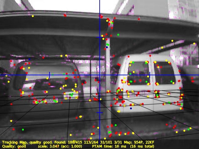
λ∗ λ∗x λ∗y arith. mean geo. mean median zI,t is hence given by
3
ẋt cos Ψt − ẏt sin Ψt
estimated scale
2.5 ẋt sin Ψt + ẏt cos Ψt
2
żt
hI (xt ) :=
(9)
Φt
1.5 Θt
0 1 2 3 4
10 10 10 10 10 Ψ̇t
number of samples
zI,t := (v̂x,t , v̂y,t , (ĥt − ĥt−1 ), Φ̂t , Θ̂t , (Ψ̂t − Ψ̂t−1 ))T (10)
Fig. 4. Comparison of λ∗ with Other Estimators: The plot shows the
estimated scale as more samples are added. It can be seen that the proposed
estimator λ∗ is the only consistent estimator, i.e., the only one converging 2) Visual Observation Model: When PTAM success-
to the correct value. For this plot we used λ = 2, σx = 1, σy = 0.3 and fully tracks a video frame, we scale the pose estimate by
µi ∼ N (03 , 13×3 ). the current estimate for the scaling factor λ∗ and transform
it from the coordinate system of the front camera to the
2) λ∗ → λ∗x for σx2 → 0, and λ∗ → λ∗y for σy2 → 0, i.e., these coordinate system of the quadrocopter, leading to a direct
naı̈ve estimators correspond to the case when one of observation of the quadrocopter’s pose given by
the measurement sources is noise-free.
hP (xt ) := (xt , yt , zt , Φt , Θt , Ψt )T (11)
We extensively tested our approach on artificially generated
zP,t := f (EDC EC ,t ) (12)
data according to (2) and compared it to other, simple
estimators, that is the arithmetic mean, geometric mean and where EC ,t ∈ SE(3) is the estimated camera pose (scaled with
the median of the set of quotients kx ik
kyi k . It can be observed λ ), EDC ∈ SE(3) the constant transformation from the camera
that out of all presented possibilities, our approach is the only to the quadrocopter coordinate system, and f : SE(3) → R6
consistent estimator, i.e., the only one converging to the true the transformation from an element of SE(3) to our roll-
scale for all dimensions d, values for σx2 , σy2 and values for pitch-yaw representation.
µi . An example is shown in Fig. 4. Furthermore, λ∗ can be 3) Prediction Model: The prediction model describes
computed efficiently, as each new sample pair only requires how the state vector xt evolves from one time step to the next.
one update of the three sums, and the re-evaluation (7). Note In particular, we approximate the quadrocopter’s horizontal
that in practice approximations for σx2 and σy2 are sufficient, acceleration ẍ, ÿ based on its current state xt , and estimate
as their influence on λ∗ decreases rapidly the more accurate its vertical acceleration z̈, yaw-rotational acceleration Ψ̈ and
the measured distances are. More results on the accuracy of roll/pitch rotational speed Φ̇, Θ̇ based on the state xt and the
this method will be presented in Section V-A. active control command ut .
The horizontal acceleration is proportional to the horizon-
B. State Prediction and Observation tal force acting upon the quadrocopter, which is given by
In this section, we describe the state space, the observation ẍ
∝ facc − fdrag (13)
models and the motion model used in the EKF. The state ÿ
space consists of a total of ten state variables
where fdrag denotes the drag and facc denotes the accelerating
force. The drag is approximately proportional to the horizon-
xt := (xt , yt , zt , ẋt , ẏt , żt , Φt , Θt , Ψt , Ψ̇t )T ∈ R10 , (8) tal velocity of the quadrocopter, while facc depends on the
tilt angle. We approximate it by projecting the quadrocopter’s
where (xt , yt , zt ) denotes the position of the quadrocopter in z-axis onto the horizontal plane, which leads to
m and (ẋt , ẏt , żt ) the velocity in m/s, both in world coordinates.
Further, the state contains the roll Φt , pitch Θt and yaw Ψt ẍ(xt ) = c1 (cos Ψt sin Φt cos Θt − sin Ψt sin Θt ) − c2 ẋt (14)
angle of the drone in deg, as well as the yaw-rotational speed ÿ(xt ) = c1 (− sin Ψt sin Φt cos Θt − cos Ψt sin Θt ) − c2 ẏt (15)
Ψ̇t in deg/s. In the following, we define for each sensor an
observation function h(xt ) and describe how the respective We estimated the proportionality coefficients c1 and c2 from
observation vector zt is composed from the sensor readings. data collected in a series of test flights. Note that this model
1) Odometry Observation Model: The quadrocopter assumes that the overall thrust generated by the four rotors
measures its horizontal speed v̂x,t and v̂y,t in its local co- is constant. Furthermore, we describe the influence of sent
ordinate system, which we transform into the global frame ¯ ) by a linear model:
control commands ut = (Φ̄t , Θ̄t , ż¯t , Ψ̇t
ẋt and ẏt . The roll and pitch angles Φ̂t and Θ̂t measured by
the accelerometer are direct observations of Φt and Θt . To Φ̇(xt , ut ) = c3 Φ̄t − c4 Φt (16)
account for yaw-drift and uneven ground, we differentiate Θ̇(xt , ut ) = c3 Θ̄t − c4 Θt (17)
the height measurements ĥt and yaw measurements Ψ̂t and ¯ − c Ψ̇
Ψ̈(x , u ) = c Ψ̇
t t 5 t 6 t (18)
treat them as observations of the respective velocities. The
resulting observation function hI (xt ) and measurement vector z̈(xt , ut ) = c7 ż¯t − c8 żt (19)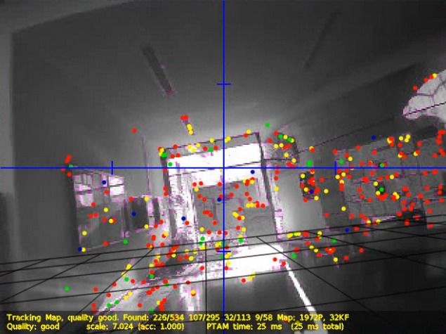
vertical motion horizontal motion
Again, we estimated the coefficients c3 , . . . , c8 from test flight 2.5 2.5
estimated length of 1 m [m]
data. The overall state transition function is now given by
xt+1 xt ẋt 2 2
yt+1 yt ẏt
zt+1 zt żt 1.5 1.5
ẋt+1 ẋt ẍ(xt )
← + δt ÿ(xt )
ẏt+1 ẏt
żt+1 żt z̈(xt , ut ) (20) 1 1
Φt+1 Φt Φ̇(xt , ut ) 0 5 10 15 20 0 5 10 15 20
time [s] time [s]
Θt+1 Θt Θ̇(xt , ut )
Ψt+1 Ψt Ψ̇t Fig. 6. Scale Estimation Accuracy: The plots show the mean and standard
deviation of the the estimation error e, corresponding to the estimated length
Ψ̇t+1 Ψ̇t Ψ̈(xt , ut ) of 1 m, from horizontal and vertical motion. It can be seen that the scale
can be estimated accurately in both cases, it is however more accurate and
using the model specified in (14) to (19). Note that, due to converges faster if the quadrocopter moves vertically.
the many assumptions made, we do not claim the physical
correctness of this model. It however performs very well ground truth delayed ground truth prediction
in practice, which is mainly due to its completeness: the 2
behavior of all state parameters and the effect of all control
commands is approximated, allowing “blind” prediction, i.e., 0
x [m]
prediction without observations for a brief period of time
(∼ 125 ms in practice, see Fig. 3). −2
0 1 2 3 4 5 6 7
1
V. E XPERIMENTS AND R ESULTS
0
ẋ [m/s]
We conducted a series of real-world experiments to ana- −1
lyze the properties of the resulting system. The experiments −2
were conducted in different environments, i.e., both indoor 0 1 2 3 4 5 6 7
in rooms of varying size and visual appearance as well as time [s]
outdoor under the influence of sunlight and wind. A selection Fig. 7. Comparison of Predicted and Real State. The black curve
shows the ground truth, it can only be computed with a delay of ∼ 250 ms
of these environments is depicted in Fig. 5. (dashed curve). At t = 5 s, the quadrocopter is manually pushed away which
In the following, we present our results on the convergence cannot be predicted – hence the brief deviation. This plot shows (1) that
behavior and accuracy of scale estimation in Section IV- the prediction approximates the ground truth well and in particular without
notable delay and (2) that using visual information, the EKF rapidly recovers
A, the accuracy of the motion model in Section V-B, the from large external disturbances – however with a small delay.
responsiveness and accuracy of pose control in Section V-C,
and the long-term stability and drift elimination in Section V-
D. mean feature depth in meters of the first keyframe, which in
As ground truth at time t we use the state of the EKF after our experiments ranges from 2 m to 10 m. To provide better
all odometry and visual pose information up to t have been comparability, we analyze and visualize the estimation error
∗
received and integrated. It can only be calculated at t + ∆tvis , e := λ , corresponding to the estimated length of 1 m.
λ̂
and therefore is not used for drone control – in practice it is Fig. 6 gives the mean error as well as the standard
available ∼ 250 ms after a control command for t has been deviation spread over 10 flights. As can be seen, our method
computed and sent to the quadrocopter. quickly and accurately estimates the scale from both types
of motion. Due to the superior accuracy of the altimeter
A. Scale Estimation Accuracy compared to the horizontal velocity estimates, the estimate
To analyze the accuracy of the scale estimation method converges faster and is more accurate if the quadrocopter
derived in IV-A, we instructed the quadrocopter to fly a moves vertically, i.e., convergence after 2 s versus 15 s, and
fixed figure, while every second a new sample is taken to a final accuracy ±1.7 % versus ±5 %. Note that in practice,
and the scale re-estimated. In the first set of flights, the we allow for (and recommend) arbitrary motions during scale
quadrocopter was commanded to move only vertically, such estimation so that information from both sensor modalities
that the samples mostly consist of altitude measurements. can be used to improve convergence. Large, sudden changes
In the second set, the quadrocopter was commanded to fly in measured relative height can be attributed to uneven
a horizontal rectangle, such that primarily the IMU-based ground, and removed automatically from the data set.
velocity information is used. After each flight, we measured
the ground truth λ̂ by manually placing the quadrocopter at B. State Prediction Accuracy
two measurement points, and comparing the known distance In this section we give a qualitative evaluation of the
between these points with the distance measured by the accuracy of the predicted state of the quadrocopter, used
visual SLAM system. Note that due to the initial scale for control. Fig. 7 shows both the predicted state for time
normalization, the values for λ̂ roughly correspond to the t as well as the ground truth, i.e., the state computed after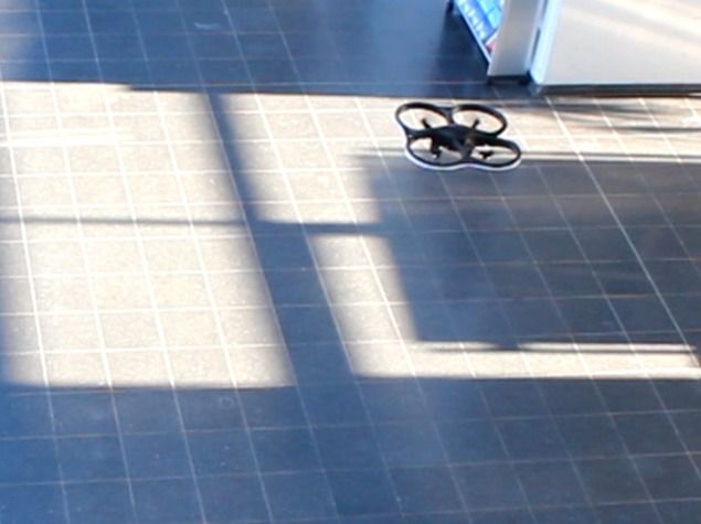
small office kitchen large office large indoor area outdoor
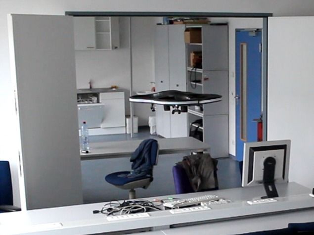
Fig. 5. Testing Environments: The top row shows an image of the quadrocopter flying, the bottom row the corresponding image from the quadrocopter’s
frontal camera. This shows that our system can operate robustly in different, real-world environments.
TABLE I
x [m] // sent control
2 setpoint
C ONVERGENCE S PEED IN P OSITION C ONTROL state
sent control
1 P control
relative motion (x, y, z) [m] (1,0,0) (4,0,0) (0,0,1) (1,1,1) D control
0
tconv [s] 3.1 ± 1.3 4.5 ± 0.8 3.1 ± 0.1 3.9 ± 0.5
−1
−2
all sensor measurements have been evaluated. This is only
−1 0 1 2 3 4 5 6 7 8 9
possible ∼ 250 ms after the respective control command time [s]
has been issued. It can be observed that the prediction
Fig. 8. Flying a Large Distance: The plot shows the behavior of the
approximates the ground truth very well and without notable controller for a large distance. As can be seen, the quadrocopter accelerates
delay, which is crucial for oscillation-free control. with maximum pitch for the first second and decelerates before converging
on the setpoint.
C. Positioning Accuracy and Convergence Speed
setpoint state sent control
In this Section, we evaluated the performance of the
1
complete system in terms of position control. In particular,
x [m]
we measured the average time to approach a given goal 0
tconv tconv
location and the average positioning error while holding −1
0 5 10 15 20 25
this position. Considering the large delay in our system, 1
y [m]
the pose stability of the quadrocopter heavily depends on 0
an accurate prediction from the EKF: the more accurate the tconv tconv
−1
pose estimates and in particular the velocity estimates are, 0 5 10 15 20 25
1
the higher the gains can be set without leading to oscillations.
z [m]
To determine the stability, we instructed the quadrocopter 0
tconv tconv
to hold a target position over 60 s in different environments −1
0 5 10 15 20 25
and measure the root mean square error (RMSE). The results time [s]
fly to fly to fly to fly to
are given in Fig. 10: the measured RMSE lies between 4.9 cm (1,0,0) (1,1,0) (1,1,1) (0,0,0)
(indoor) and 18.0 cm (outdoor). Fig. 9. Example Flight: Flying a simple figure consisting of four
To evaluate the convergence speed, we repeatedly let the waypoints. This plot illustrates the typical behavior of the quadrocopter
quadrocopter fly a given distance and measure the con- when holding and approaching waypoints (tconv is indicated, see also Tab. I).
vergence time tconv , corresponding to the time required to kitchen large indoor area outdoor
reach the target position and hold it for at least 5 s. We RMSE = 4.9 cm RMSE = 7.8 cm RMSE = 18.0 cm
consider the quadrocopter to be at the target position if the
0.4 0.4 0.4
Euclidean distance is less than 10 cm. An example of flying 0.2 0.2 0.2
y [m]
0 0 0
a long distance in x-direction is shown in Fig. 8: the plot −0.2 −0.2 −0.2
clearly shows that the quadrocopter accelerates initially with −0.4 −0.4 −0.4
0.4 0.4 0.4
maximum pitch, and de-accelerates before reaching the target 0 0
0.4
0 0
0.4
0 0
0.4
location at t = 3.5 s. Fig. 9 shows an example trajectory in all y [m] −0.4 −0.4 x [m] y [m] −0.4 −0.4 x [m] y [m] −0.4 −0.4 x [m]
three dimensions. We repeated this experiment ten times and Fig. 10. Flight Stability: Path taken and RMSE of the quadrocopter when
summarized the results in Tab. I. Reaching a target location instructed to hold a target position for 60 s, in three of the environments
at a distance of 4 m took on average 4.5 s. depicted in Fig. 5. It can be seen that the quadrocopter can hold a position
very accurately, even when perturbed by wind (right).
EKF trajectory           raw odometry              target trajectory   experiments in different real-world indoor and outdoor en-
                                                                                       vironments. With these experiments, we demonstrated that
            3                                                                          accurate, robust and drift-free visual navigation is feasible
                                                2
                                                                                       even with low-cost robotic hardware.
            2
                                                0
                                                                                                                     R EFERENCES
   y [m]

            1                                  −2
                                                                                        [1] D. Mellinger and V. Kumar, “Minimum snap trajectory generation
            0                                  −4                                           and control for quadrotors,” in Proc. IEEE Intl. Conf. on Robotics
                                                                                            and Automation (ICRA), 2011.
                                               −6                                       [2] S. Lupashin, A. Schöllig, M. Sherback, and R. D’Andrea, “A sim-
           −1
                                                                                            ple learning strategy for high-speed quadrocopter multi-flips.” in
                                               −8                                           Proc. IEEE Intl. Conf. on Robotics and Automation (ICRA), 2010.
                 −1     0        1   2     3        −8   −6   −4     −2    0    2       [3] M. Müller, S. Lupashin, and R. D’Andrea, “Quadrocopter ball jug-
                            x [m]                                  x [m]                    gling,” in Proc. IEEE Intl. Conf. on Intelligent Robots and Systems
Fig. 11. Elimination of Odometry Drift: Horizontal path taken by the                        (IROS), 2011.
quadrocopter as estimated by the EKF compared to the raw odometry (i.e.,                [4] Q. Lindsey, D. Mellinger, and V. Kumar, “Construction of cubic
the integrated velocity estimates). Left: when flying a figure; right: when                 structures with quadrotor teams,” in Proceedings of Robotics: Science
being pushed away repeatedly from its target position. The odometry drift                   and Systems (RSS), Los Angeles, CA, USA, 2011.
is clearly visible, in particular when the quadrocopter is being pushed away.           [5] S. Grzonka, G. Grisetti, and W. Burgard, “Towards a navigation system
When incorporating visual pose estimates, it is eliminated completely.                      for autonomous indoor flying,” in Proc. IEEE Intl. Conf. on Robotics
                                                                                            and Automation (ICRA), 2009.
                                                                                        [6] M. Blösch, S. Weiss, D. Scaramuzza, and R. Siegwart, “Vision based
D. Drift Elimination                                                                        MAV navigation in unknown and unstructured environments,” in
                                                                                            Proc. IEEE Intl. Conf. on Robotics and Automation (ICRA), 2010.
   To verify that the incorporation of a visual SLAM sys-                               [7] M. Achtelik, M. Achtelik, S. Weiss, and R. Siegwart, “Onboard IMU
tem eliminates odometry drift, we compare the estimated                                     and monocular vision based control for MAVs in unknown in- and
trajectory with and without the visual SLAM system. Fig. 11                                 outdoor environments,” in Proc. IEEE Intl. Conf. on Robotics and
                                                                                            Automation (ICRA), 2011.
shows the resulting paths, both for flying a fixed figure (left)                        [8] M. Achtelik, A. Bachrach, R. He, S. Prentice, and N. Roy, “Stereo
and for holding a target position while the quadrocopter is                                 vision and laser odometry for autonomous helicopters in GPS-denied
being pushed away (right). Both flights took approximately                                  indoor environments,” in Proc. SPIE Unmanned Systems Technology
                                                                                            XI, 2009.
35 s, and the quadrocopter landed no more than 15 cm away                               [9] A. S. Huang, A. Bachrach, P. Henry, M. Krainin, D. Maturana, D. Fox,
from its takeoff position. In contrast, the raw odometry                                    and N. Roy, “Visual odometry and mapping for autonomous flight
accumulated an error of 2.1 m for the fixed figure and 6 m                                  using an RGB-D camera,” in Proc. IEEE International Symposium of
                                                                                            Robotics Research (ISRR), 2011.
when being pushed away. This experiment demonstrates that                              [10] D. Mellinger, N. Michael, and V. Kumar, “Trajectory generation
the visual SLAM system efficiently eliminates pose drift                                    and control for precise aggressive maneuvers with quadrotors,” in
during maneuvering.                                                                         Proceedings of the Intl. Symposium on Experimental Robotics, Dec
                                                                                            2010.
E. Robustness to Temporary Loss of Visual Tracking                                     [11] D. Eberli, D. Scaramuzza, S. Weiss, and R. Siegwart, “Vision based
                                                                                            position control for MAVs using one single circular landmark,” Journal
   The system as a whole is robust to temporary loss of                                     of Intelligent and Robotic Systems, vol. 61, pp. 495–512, 2011.
visual tracking, e.g. due to occlusions or large rotations, as it                      [12] T. Krajnı́k, V. Vonásek, D. Fišer, and J. Faigl, “AR-drone as a platform
                                                                                            for robotic research and education,” in Proc. Research and Education
continues to navigate based only on odometry measurements.                                  in Robotics: EUROBOT 2011, 2011.
As soon as visual tracking recovers, the EKF state is updated                          [13] “Ascending technologies,” 2012. [Online]: http://www.asctec.de/
with the absolute pose estimate, eliminating accumulated                               [14] M. Blösch, S. Weiss, D. Scaramuzza, and R. Siegwart, “Vision based
                                                                                            MAV navigation in unknown and unstructured environments,” in
estimation error. This is demonstrated in the attached video.                               Proc. IEEE Intl. Conf. on Robotics and Automation (ICRA), 2010.
                                                                                       [15] S. Zingg, D. Scaramuzza, S. Weiss, and R. Siegwart, “MAV navi-
                      VI. C ONCLUSION                                                       gation through indoor corridors using optical flow,” in Proc. IEEE
   In this paper, we presented a visual navigation system for a                             Intl. Conf. on Robotics and Automation (ICRA), 2010.
                                                                                       [16] “Parrot AR.Drone,” 2012. [Online]: http://ardrone.parrot.com/
low-cost quadrocopter using offboard processing. Our system                            [17] S. Weiss, M. Achtelik, M. Chli, and R. Siegwart, “Versatile distributed
enables the quadrocopter to visually navigate in unstructured,                              pose estimation and sensor self-calibration for an autonomous mav,”
GPS-denied environments and does not require artificial                                     in Proc. IEEE Intl. Conf. on Robotics and Automation (ICRA), 2012.
                                                                                       [18] G. Nützi, S. Weiss, D. Scaramuzza, and R. Siegwart, “Fusion of IMU
landmarks nor prior knowledge about the environment. The                                    and vision for absolute scale estimation in monocular SLAM,” Journal
contribution of this paper is two-fold: first, we presented                                 of Intelligent Robotic Systems, vol. 61, pp. 287 – 299, 2010.
a robust solution for visual navigation with a low-cost                                [19] C. Bills, J. Chen, and A. Saxena, “Autonomous MAV flight in indoor
                                                                                            environments using single image perspective cues,” in Proc. IEEE
quadrocopter. Second, we derived a maximum-likelihood                                       Intl. Conf. on Robotics and Automation (ICRA), 2011.
estimator in closed-form to recover the absolute scale of the                          [20] T. Krajnı́k, V. Vonásek, D. Fišer, and J. Faigl, “AR-drone as a platform
visual map, providing an efficient and consistent alternative                               for robotic research and education,” in Proc. Communications in
                                                                                            Computer and Information Science (CCIS), 2011.
to predominant filtering-based methods. Our system was able                            [21] W. S. Ng and E. Sharlin, “Collocated interaction with flying robots,”
to estimate the map scale up to ±1.7% of its true value,                                    in Proc. IEEE Intl. Symposium on Robot and Human Interactive
with which we achieved an average positioning accuracy                                      Communication, 2011.
                                                                                       [22] G. Klein and D. Murray, “Parallel tracking and mapping for small AR
of 4.9 cm (indoor) to 18.0 cm (outdoor). Furthermore, our                                   workspaces,” in Proc. IEEE Intl. Symposium on Mixed and Augmented
approach is able to robustly deal with communication delays                                 Reality (ISMAR), 2007.
of up to 400 ms. We tested our system in a set of extensive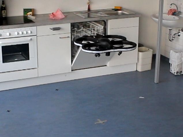
You can also read