A Holistic Motion Planning and Control Solution to Challenge a Professional Racecar Driver
←
→
Page content transcription
If your browser does not render page correctly, please read the page content below
IEEE ROBOTICS AND AUTOMATION LETTERS. PREPRINT VERSION. ACCEPTED JULY, 2021                                                                              1

                                             A Holistic Motion Planning and Control Solution
                                               to Challenge a Professional Racecar Driver
                                                                         Sirish Srinivasan∗ , Sebastian Nicolas Giles∗ , Alexander Liniger

                                            Abstract—We present a holistically designed three layer control
                                         architecture capable of outperforming a professional driver
                                         racing the same car. Our approach focuses on the co-design
arXiv:2103.00358v2 [cs.RO] 19 Aug 2021

                                         of the motion planning and control layers, extracting the full
                                         potential of the connected system. First, a high-level planner
                                         computes an optimal trajectory around the track, then in real-
                                         time a mid-level nonlinear model predictive controller follows
                                         this path using the high-level information as guidance. Finally
                                         a high frequency, low-level controller tracks the states predicted
                                         by the mid-level controller. Tracking the predicted behavior has
                                         two advantages: it reduces the mismatch between the model                      Fig. 1. pilatus driverless, the formula student race car ©FSG - Schulz.
                                         used in the upper layers and the real car, and allows for a
                                         torque vectoring command to be optimized by the higher level
                                         motion planners. The tailored design of the low-level controller
                                         proved to be crucial for bridging the gap between planning and                 higher driving performance and lower lap times than a profes-
                                         control, unlocking unseen performance in autonomous racing.                    sional racecar driver, both driving the same Formula Student
                                         The proposed approach was verified on a full size racecar,                     Driverless car developed by AMZ Racing, from ETH Zürich.
                                         considerably improving over the state-of-the-art results achieved
                                         on the same vehicle. Finally, we also show that the proposed                      Most autonomous racing motion planners and controllers
                                         co-design approach outperforms a professional racecar driver.                  can be divided into three levels. The first level is track-level
                                            Index Terms—Motion and Path Planning, Field Robots, Intel-                  planning, where the race line around the track is determined.
                                         ligent Transportation Systems.                                                 This can be done using either lap-time optimization methods
                                                                                                                        [8]–[10], or using the center line [7], [11], [12]. The mid-level
                                                                                                                        is tasked to follow the track-level path, and is normally based
                                                                   I. I NTRODUCTION                                     on two common approaches - static feedback controllers [6],
                                                                                                                        [13], [14] or online optimization-based methods [7], [15]–[17]
                                               UTONOMOUS driving has progressed massively over
                                         A     past few decades, from its humble beginnings in the
                                         1980s [1], [2], over the DARPA challenges [3], [4], to the
                                                                                                                        such as Nonlinear Model Predictive Control (NMPC). The last
                                                                                                                        level is the Low-Level vehicle Control (LLC) which handles
                                                                                                                        steering and stability control, and typically hosts torque vec-
                                         self-driving car companies of today. One goal for autonomous                   toring algorithms which are also beneficial for a human driver
                                         driving has always been to surpass human driving capabilities.                 [18]. Even though this layer is fundamental, it is often under-
                                         This is especially true for autonomous racing, where profes-                   explored, especially the coupling with the mid-level. There
                                         sional racecar drivers are a challenging benchmark. However,                   exist several works that make use of a sophisticated LLC.
                                         most existing methods fall short of this goal [5]. In the last                 However, these are either designed for human drivers [10], [11]
                                         years, several motion planning methods for autonomous racing                   or do not exploit that the level above is an automatic controller
                                         have emerged [6], [7]. In this paper, we introduce a holistic                  [14], [19]. In this work, we show that co-designing the LLC to
                                         view-point on motion planning and control of autonomous                        work in harmony with the higher levels allows improving the
                                         racecars, and show that the co-design of all layers from track-                performance of the autonomous racecar drastically. We achieve
                                         level trajectory planning to low-level control of the vehicle                  this by tracking parts of the mid-level NMPC state trajectory
                                         dynamics results in an unseen performance on a full-sized                      with the LLC. This reinforces recent work which showed that
                                         autonomous racecar. In fact our proposed approach achieves                     better coupling the track and mid-level controllers [10], [20]
                                                                                                                        can improve the performance, and [19] that highlighted the
                                            Manuscript received: February, 24, 2021; Revised June, 11, 2021; Accepted   benefits of torque vectoring for autonomous cars.
                                         July, 14, 2021. This paper was recommended for publication by Editor Stephen
                                         J. Guy upon evaluation of the Associate Editor and Reviewers’ comments.           A different view point supporting the coupling of different
                                            Sirish Srinivasan and Sebastian Nicolas Giles are with AMZ Driver-          levels is based on model mismatch. Several papers discovered
                                         less, ETH Zürich, 8092 Zürich, Switzerland (e-mail: sirishs@ethz.ch;         model mismatch as a crucial issue in autonomous racing - the
                                         sgiles@ethz.ch)
                                            Alexander Liniger is with the Computer Vision Lab, ETH Zürich, 8092        problem arises due to the relatively simple models used in
                                         Zürich, Switzerland (e-mail: alex.liniger@vision.ee.ethz.ch)                  most autonomous racing stacks. Solutions range from using
                                            ∗ The authors contributed equally to this work.
                                                                                                                        complex models [20], stochastic MPC [21], to NMPC with
                                            A supplementary video providing a high level overview of the approach,
                                         along with a demonstration of the experimental results is available.           model learning [22], [23] to learn the model mismatch. All
                                            Digital Object Identifier (DOI): see top of this page.                      these methods tackle the problem in the mid-level and come
2                                                       IEEE ROBOTICS AND AUTOMATION LETTERS. PREPRINT VERSION. ACCEPTED JULY, 2021

with drawbacks in terms of the computational load. However,         for significant freedom in its design. Going beyond basic
using our co-design approach, we can use the LLC to make            wheel torque distribution and stabilization [11], [24], we
the real-car behave closer to the model of the NMPC.                define a novel input interface for our LLC, consisting of the
   In this paper we extend the approach proposed in [10] and        desired short-term trajectories of key vehicle states, namely
highlight the importance of properly coupled high and low-          the longitudinal acceleration āx , yaw rate r̄ and steering angle
level controllers. Our contributions are threefold:                 δ̄. Note that a bar on top of a variable denotes a target, while
   • We propose a new low-level controller (LLC) designed           no bar refers to the actual variable. Importantly, the drive
      to distribute the motor torques of our all-wheel drive race   force and torque vectoring commands used by the NMPC
      car to reduce the model mismatch between the real car         and described in Section IV-A are purely virtual and are
      and the model used in the higher level layers.                not directly passed to the LLC. This is the fundamental idea
   • We propose to directly optimize over a torque vectoring        for our high-level to low-level coupling: the state predictions
      input in the higher level controllers, while interfacing it   by the NMPC are processed and passed to the LLC which
      with the LLC in terms of a yaw-rate target trajectory.        appropriately commands the individual actuators to reproduce
      This allows to extract the full potential out of our LLC.     them. The low-level feedback loop actively makes the car
   • We show that the proposed framework can drastically            behave more like the NMPC model, mitigating the effect of
      improve the performance over the current state-of-the-art     model mismatch in the NMPC.
      autonomous racing systems, both in simulation and exper-
      iments. In fact our method is the first which performs on     A. Wheel Torque Controller
      par with a professional racecar driver, even outperforming
      the driver in our experimental setup.                             The LLC operates at 200Hz, significantly faster than the
                                                                    40Hz of the upper level NMPC which sends the target tra-
In this work, attention is given to the LLC formulation and its
                                                                    jectories. To exploit the higher bandwidth, we generate in-
coupling with the upper control layers, complementing [10]
                                                                    between target values using linear up-sampling of the MPC
which focused on the high and mid-level and their coupling.
                                                                    target trajectories. We correct for the delay in the robotic
This is also the main difference to other NMPC-based methods
                                                                    system by slightly shifting the target points in time.
[7], [12], [17] which do not focus on the LLC or torque
vectoring. With respect to other works that considered LLC,             The LLC computes the torques of the four wheels in a
ours is distinguished by the novel interface between the levels:    two step approach. First, the required yaw moment and total
in [10], [11], [19], [24] the low-level targets are mainly          torque are determined. Second, the individual wheel torques
determined by the steering angle, in contrast, we incorporate       are computed fulfilling these requirements.
the yaw rate of the mid-level NMPC. In [6], [14], the focus             The yaw moment is computed using a proportional con-
is on traction control which is a subtask of our LLC.               troller to track the target yaw rate τz = KP (r̄ − r). The total
                                                                    torque demand is computed using a PID-controller for the
                                                                    target longitudinal acceleration as τtotal = P ID(āx − ax ) +
     II. C O - DESIGNED C ONTROLLER A RCHITECTURE
                                                                    māx + q, where the feed forward part is designed such that m
   As discussed in the introduction, we build upon [10] but         approximates the inertia of the vehicle including the drive train
introduce several fundamental changes highlighted in our first      and q the effect of drag. The computation of τz and τtotal is the
two contributions. However, we keep a similar architecture for      main difference to the LLC used in [10] and by the human
the track and mid-level layers, which are the focus of [10]. Our    driver in Section VI-D where the steering angle is used to
full architecture is shown in Figure 2. We assume a reference       compute the target yaw rate [25], and the driver command is
path from a mapping run and offline compute an optimal              directly mapped to the total torque demand.
trajectory around the track using our Trajectory Optimization           An initial torque distribution is then computed by splitting
(TRO) module. This path is then followed by the MPC-Curv            the total torque τtotal equally between the left and right sides of
module, using the terminal velocity constraint from the TRO         the car. Further, the individual torques are scaled proportional
module. However, in contrast to [10], the optimal solution          to the normal force Fz on each wheel, resulting in τ 0 =
from MPC-Curv is then translated to set point trajectories for      [τF0 L , τF0 R , τRL
                                                                                      0     0
                                                                                         , τRR ]. The torque vectoring algorithm then
the acceleration, yaw rate and steering, which are tracked using    determines the torque differences ∆τF and ∆τR , which adjusts
our new LLC. At the same time, the redeveloped vehicle model        the wheel torques to τ = τ 0 +[∆τF , −∆τF , ∆τR , −∆τR ]. The
makes the motion planning levels aware of the torque vectoring      torque differences ∆τF and ∆τR are computed such that the
capability of the car and enables optimization over a new yaw       desired yaw moment τz is produced, accounting for the effect
moment command. In addition to these two main differences           of the drive force of the angled front wheels. Since the torque
from [10], we also modify the TRO and MPC-Curv modules,             difference neglects the load distribution, in a final step, ∆τF
resulting in a drastically improved driving performance.            and ∆τR are distributed proportional to the vertical tire load
                                                                    on each axle. This allows, for example, to use mainly the rear
            III. L OW L EVEL C ONTROL D ESIGN                       wheels for torque vectoring during a corner exit.
   Our fully autonomous racecar (see Section VI-A for com-              The resulting wheel torques are finally tracked by a drive
plete specifications) is equipped with four wheelhub motors         motor controller operating at 1kHz which also implements a
that can be controlled independently. Computing the references      traction controller to adapt the reference torque if a slip-ratio-
for each motor creates the need for a LLC, but also allows          based wheel speed range is violated [26].
SRINIVASAN et al.: A HOLISTIC MOTION PLANNING AND CONTROL SOLUTION TO CHALLENGE A PROFESSIONAL RACECAR DRIVER 3
Offline Online
Steering
Linear
Reference controller
upsampling
track Yaw rate
controller
Trajectory MPC-Curv
Acceleration Total torque Torque
optimization controller distribution Vectoring
Fig. 2. Full planning and control architecture. The feedback from the state estimator is omitted for simplicity.
B. Steering delay compensation module levels. We follow the popular modeling approach successfully
The position tracking delay of a servo steering system, due used in [7], [10], [11], and uses a dynamic bicycle model
to mechanical compliance and limited power, can severely hin- with Pacejka tire models. Compared to [10] we include some
der driving. To mitigate this we propose a virtual target point important differences - first we assume that the force of the
δ̄act as a reference for the steering positioning actuator, based motors FM can be directly controlled, and for simplicity
on an external steering shaft sensor measurement δ. The virtual assume that the same motor force is applied at the front and
target point is estimated as δ̄act = δ̄ + KP (δ̄ − δ) + KD (δ̄˙ − δ̇), rear wheels. This approach is better aligned with our LLC,
˙ which is designed to track an acceleration target and does not
where δ̄(t) is the steering rate from the MPC predictions.
expect a driver command as in [10]. Second, we introduce the
IV. M ODEL torque vectoring moment Mtv as an input. This is in contrast
to [10], [11] where the torque vectoring was determined by a
Given the LLC, we introduce the vehicle model used in the simple P-controller. This input is fundamental, as it allows
higher level motion planners. Similar to [10] we formulate the higher level controllers to fully utilize the torque vec-
a dynamic bicycle model in curvilinear coordinates, but we toring capabilities, going beyond a simple rule-based method
modify the interface with our LLC (See Section III). designed for human drivers. We use a state lifting technique
to consider input rates, but do not lift Mtv to allow the high
A. Curvilinear Dynamic Bicycle Model level controllers to use the torque vectoring for highly transient
Curvilinear coordinates describe a coordinate frame (Frenet situations. The state is given by x̃ = [s, n, µ, vx , vy , r, FM , δ]T
frame) formulated locally with respect to a reference path, and the input as u = [∆FM , ∆δ, Mtv ]T . Resulting in the
drastically simplifies path following formulations. In our case following system dynamics,
the reference path can be the center line or the track-level vx cos µ − vy sin µ
optimized path. The kinematic states in the curvilinear setting ṡ = ,
1 − nκ(s)
describe the state relative to the reference path and are the
progress along the path s, the deviation orthogonal to the path ṅ = vx sin µ + vy cos µ ,
n, and the local heading µ. Note that the dynamic states are not µ̇ = r − κ(s)ṡ , (1)
influenced by the change in the coordinate system, and in our 1
v̇x = m (FM (1 + cos δ) − Fy,F sin δ + mvy r − Ffric ) ,
model we consider the longitudinal vx and lateral velocities vy , v̇y = m 1
(Fy,R + FM sin δ + Fy,F cos δ − mvx r) ,
and yaw rate r. A visualization of the curvilinear coordinates 1
as well as the other states is shown in Figure 3. ṙ = Iz ((FM sin δ + Fy,F cos δ)lF − Fy,R lR + Mtv ) ,
ḞM = ∆FM ,
δ̇ = ∆δ ,
where lF and lR are the distances from the Center of Gravity
(CoG) to the front and rear wheels respectively, m is the mass
of the vehicle and Iz the moment of inertia. Finally, κ(s) is the
curvature of the reference path at the progress s. We denote
the dynamics in (1) as x̃˙ = ftc (x̃, u), where the superscript
c highlights that it is a continuous model and the subscript t
that it is a time-domain model.
The lateral forces at the front Fy,F and rear Fy,R tires are
modeled using a simplified Pacejka tire model [27],
Fy,F = FN,F D sin (C arctan (BαF )) ,
Fig. 3. Visualization of the curvilinear coordinates (blue), as well as the (2)
dynamic states (green) and the forces (red). Fy,R = FN,R D sin (C arctan (BαR )) ,
v +l r v −l r
Since the LLC handles traction control and considering load where αF = arctan ( y vxF ) − δ and αR = arctan ( y vxR )
changes, we can use a relatively simple model in our higher are the slip angles at the front and rear wheels respectively, and4 IEEE ROBOTICS AND AUTOMATION LETTERS. PREPRINT VERSION. ACCEPTED JULY, 2021
B, C and D are the parameters of the simplified Pacejka tire necessary to optimize for a periodic trajectory. Thus, we add
model. The net normal load FN,net = mg +Cl vx2 , where Cl is a periodicity constraint fsd (xN , uN ) = x0 , where N is the
a lumped lift coefficient. Compared to [10] we also consider number of discretization steps.
the aerodynamic downforce, which is important since we push The cost function seeks to maximize the progress rate ṡ,
the car to the limit of friction. The resulting normal loads on and also contains two regularization terms - a slip angle cost
the front and rear tires are given by FN,F = FN,net lR /(lF + and a penalty on the input rates. The slip angle cost penalizes
lR ) and FN,R = FN,net lF /(lF +lR ). Finally, the friction force the difference between the kinematic and dynamic side slip
Ffric is a combination of a static rolling resistance Cr and the angles as B(xk ) = qβ (βdyn,k − βkin,k )2 , where qβ > 0 is
aerodynamic drag term Cd vx2 . a weight, βkin,k = arctan(δk lR /(lF + lR )), and βdyn,k =
arctan(vy,k /vx,k ). The regularizer on the input rates is uT Ru,
B. Constraints where R is a diagonal weight matrix with positive weights. In
summary, the overall cost function is,
Similar to [10] we impose constraints to ensure that the car
remains within the track, and that we do not demand inputs JTRO (xk , uk ) = −ṡk + uT Ru + B(xk ) . (6)
that violate friction ellipse or input constraints. More precisely
Note that we introduced a new cost function compared to [10],
we have a track constraint x̃ ∈ XTrack , which is a heading-
which minimized the time. Our new cost function is nearly
dependent constraint on the lateral deviation n, and ensures
identical to the one used in the MPC-Curv motion planner
that the whole car remains inside the track [28],
(Section V-B), which makes tuning easier, and better aligns
n + Lc sin |µ| + Wc cos µ ≤ NL (s) , the solutions of the two levels.
(3)
−n + Lc sin |µ| + Wc cos µ ≤ NR (s) , Finally, we combine the cost, model and model related
constraints from Section IV-B, to formulate the trajectory
where Lc and Wc are the distances from the CoG to the optimization problem,
furthest apart corner point of the car, and NR/L (s) are the left
N
and right track width at the progress s. The tire models used X
(2) do not consider combined slip. To prevent the high level min JTRO (xk , uk )
X,U
k=0
layers to demand unrealistic accelerations from the LLC, we
limit the combined forces to remain within a friction ellipse, s.t. xk+1 = fsd (xk , uk ) ,
(7)
2 2 2 fsd (xN , uN ) = x0 ,
(ρlong FM ) + Fy,F/R ≤ (λDF/R ) , (4)
xk ∈ XTrack , xk ∈ XFE ,
where ρlong defines the shape of the ellipse, and λ determines ak ∈ A, k = 0, ..., N ,
the maximum combined force. We denote the friction ellipse
constraints in (4) by x̃ ∈ XFE . where X = [x0 , ..., xN ] and U = [u0 , ..., uN ]. The problem
Finally, we consider box constraints for both the physical is formulated using CppAD [29] and solved using Ipopt [30].
inputs and their rates. We introduce a compact notation for
all these inputs a = [FM , δ, ∆FM , ∆δ, Mtv ]T , and constrain B. MPC-Curv
them to their physical limits by the box constraint a ∈ A. We use MPC-Curv to follow the trajectory from TRO.
Since the objectives of TRO and MPC-Curv are similar, we
V. H IGH L EVEL C ONTROL F ORMULATION reuse large parts of the formulation, including the progress
A. Trajectory Optimization (TRO) rate maximization. However, since the MPC-Curv problem is
solved online, a few changes are necessary - first, we use the
Given the vehicle model and the constraints, we now
time-domain model since it is better suited for online control
focus on the higher level controllers. First the offline track-
(see [10] for a discussion). Second, since MPC-Curv has a
level trajectory optimization is described. Following [10], we
limited prediction horizon, we use the TRO solution for long
transform the continuous time dynamics (1) into the spatial
term guidance. This is done in two ways - first a regularization
domain, with progress s as the running variable instead of
cost on the lateral deviation n from the TRO path and more
time t. This transformation can be achieved as follows,
importantly a terminal velocity constraint to notify MPC-Curv
∂x̃ ∂x̃ ∂s about upcoming braking spots beyond the prediction horizon.
x̃˙ = = ,
∂t ∂s ∂t (5) To formulate the MPC-Curv problem, we first reduce the
∂x̃ 1 state to x = [n, µ, vx , vy , r, FM , δ]T . We use the initial
⇒ = ftc (x̃(s), u(s)) = fsc (x̃(s), u(s)) ,
∂s ṡ guess of s to evaluate all quantities depending on s such as
c
where fs (x̃(s), u(s)) is the continuous space model. This the curvature κ(s) outside the MPC, and hence the s-state
transformation also makes the s state redundant allowing us decouples. Second, we discretize the model using a second
to reduce the state to x = [n, µ, vx , vy , r, FM , δ]T . order Runge Kutta method, resulting in ftd (xt , ut ). In order
To formulate the track-level optimization problem, we use to decouple the prediction horizon in terms of steps and time,
the center line reference path and discretize the continuous we discretize the system with a sampling time different from
space model fsc (x(s), u(s)). An Euler forward integrator, with the update frequency of the controller. We introduce this as a
discretization ∆s is used, resulting in the discrete space system time scaling factor σ which multiplies the sampling time of
xk+1 = fsd (xk , uk ) = xk + ∆sfsc (xk , uk ). For racing, it is our controller. Note that this requires interpolating the previousSRINIVASAN et al.: A HOLISTIC MOTION PLANNING AND CONTROL SOLUTION TO CHALLENGE A PROFESSIONAL RACECAR DRIVER 5
optimal solution to get an initial guess, but at the same time C. Simulation Study
allows to predict further in time with the same horizon in steps. To highlight the benefits achieved by co-designing the high
This allows us to run MPC-Curv with higher update rates. and low-level controllers, we compare our full pipeline against
The MPC-Curv cost function is identical to the TRO (6), a modified version of it that cannot optimize over torque
with the addition of a path following cost on n, vectoring and uses the more basic LLC as in [10]. Note that
JMPC (xt , ut ) = −ṡt + qn n2t + uT Ru + B(xt ) , (8) the second method is similar to [10]. We perform a simulation
on the Formula Student Germany racetrack from 2018, using
where qn is a positive regularization weight. Thus, we can a high fidelity vehicle dynamics simulator. As an upper perfor-
now formulate the MPC-Curv problem, mance bound we also include the TRO solution, which uses
T
the dynamic bicycle model (1) with no mismatch. Figure 4
min
X
JMPC (xt , ut ) shows the longitudinal velocity vx against the progress along
X,U
t=0
the track. From the comparison, it is clearly visible that our
s.t. x0 = x̂ , approach can reach higher speeds. The lap times of the three
methods confirm this: our full system completes one lap in
xt+1 = ftd (xt , ut ) , (9)
19.9 s whilst without the low-level adaptations the lap time is
xt ∈ XTrack , xt ∈ XFE , 22.1 s, for reference, the TRO optimal lap time is 18.0 s.
at ∈ A, vx,T ≤ V̄x (sT ) ,
30
t = 0, ..., T ,
20
v x [m/s]
where the subscript t is used to highlight that the problem is 10
formulated in the time domain, and T is the prediction horizon. 0
Further, x̂ is the current curvilinear state estimate and vx,T ≤ 0 50 100 150
Track progress [m]
200 250 300
V̄x (sT ) the terminal constraint from the TRO solution. The Ours Ours w/o low-level adptations TRO
optimization problem is solved using ForcesPro [31], [32].
Fig. 4. Simulated longitudinal velocity against track position, comparing our
VI. R ESULTS AND D ISCUSSION approach with and w/o the proposed low-level adaptations, against TRO.
We first discuss our robotic platform - the autonomous
racecar pilatus driverless, followed by implementation details.
Thereafter, we benchmark our control approach in simulation D. Experimental Comparison
using a realistic vehicle simulator to study the low-level For our comparison with a professional racing driver, we
adaptations. Finally, we present experimental results including setup a race track compliant with the Formula Student Driver-
an in-depth comparison with a professional racing driver. less regulations [37], composed of sharp turns, straights and
chicanes. We tried to keep the comparison between the human
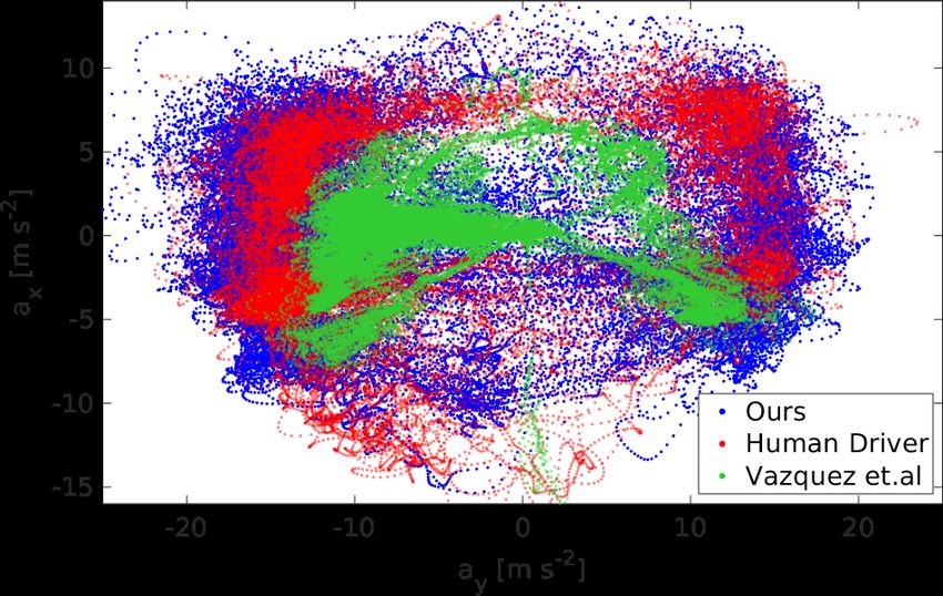
A. pilatus driverless driver and our proposed solution as fair as possible, however,
All our experiments are performed using the autonomous there are some differences. First, in autonomous mode, the car
racecar pilatus driverless (shown in Figure 1). pilatus is a is lighter due to the absence of a driver. Second, for safety, the
lightweight single seater race car, with an all-wheel drive AS speed was limited to 18 m/s, whereas the human driver was
electric powertrain. The racecar can produce ±375 Nm of unrestricted and reaches speeds up to 22 m/s. Third, the AS
torque at each wheel by means of four independent 38.4 kW can only use regenerative braking, since the hydraulic brakes
motors. Our racecar can accelerate from 0 − 100 km/h in 2.1 s are exclusively used for an emergency braking system. Since
and can reach lateral accelerations of over 20 m/s2 . pilatus is this is not necessary for the human driver, the hydraulic brakes
equipped with a complete sensor suite including two LiDARs, can also be actuated, allowing higher deceleration. We would
three cameras, an optical ground-velocity sensor and two also like to note that the steering system used by the AS is
IMUs. The low-level control as well as the state estimation slower than the steering actuated by a driver.
are deployed on an ETAS ES900 real-time embedded system; The experiments were run consecutively, with one run for
the remainder of the Autonomous System (AS), including each of the driving modes. The duration was of 12 and 18
mapping and localization, runs on an Intel Xeon E3 processor, laps for the human and AS respectively. In both cases, the car
see [11], [33]–[36] for more details. remained within the track and did not hit any cones.
1) Lap-time comparison: All of the lap times recorded
during the experiment are shown in Table I and Figure 5, no
B. TRO and MPC-Curv Implementation Details data was discarded. Our proposed controller achieves both the
TRO uses a spatial discretization of ∆s = 0.5 m. Given lowest average and minimum lap times. In Figure 5 we can see
this discretization, the optimization problem defined in (7) is that the autonomous system achieves six laps that are faster
solved in ∼ 5 s on an Intel Xeon E3 processor. We run MPC- than the fastest lap by the professional human driver. Note that
Curv at a frequency of 40Hz, with a time scaling σ = 1.5. We the variability of lap times in the autonomous mode comes
use a prediction horizon of T = 40 which results in a time from a few instances where an emergency planner is triggered
horizon of 1.5 s, using the time scaling. and automatically slows down the car to avoid leaving the6 IEEE ROBOTICS AND AUTOMATION LETTERS. PREPRINT VERSION. ACCEPTED JULY, 2021
track. This can occur during large combined slip (corner exit), our controller is able to brake later and accelerate earlier at
an issue we want to tackle in future work. several locations along the lap, which in total results in lower
lap-times, even with the top speed disadvantage.
TABLE I
L AP - TIME COMPARISON BETWEEN HUMAN AND AUTONOMOUS DRIVER
3) Inputs comparison: The low-level inputs are shown in
Figure 7. The AS in contrast to the human driver, makes
Human Autonomous limited use of the steering. This is compensated using more
Best lap-time(s) 13.62 13.39 torque vectoring, which provides a faster response of the
Mean lap-time(s) 14.19 13.95 lateral dynamics. This would not be possible without the strong
coupling at the core of our holistic architecture. Further, the
high-frequency component of the yaw moment is the intended
Human
Autonomous
effect of the LLC tracking to compensate for model mismatch.
The final difference is the relative total torque input, where
13 13.5 14 14.5 15 15.5 16
Lap time [seconds] we can see that the AS demands less torque. This is due to
the speed limit, and the fact that the friction ellipse constraint
Fig. 5. Lap-time distribution for autonomous system and human driver. limits the torque before the traction controller. The human
driver on the other hand relies on the traction controller in
Human Autonomous Timing trigger certain situations, e.g., at 100 m.
0 4) Maximum performance: Figure 8 compares the lon-
y position [m]
gitudinal and lateral accelerations recorded by the car in
-10
autonomous and human driven modes. We can see that the
-20 highest lateral, positive longitudinal and combined accelera-
-80 -70 -60 -50 -40 -30 -20 -10 0 10
x position [m]
tions are achieved by the AS. The human driver has a higher
negative longitudinal acceleration, due to the availability of
Fig. 6. GPS trajectory comparison of the best autonomous and human driven hydraulic brakes, which are not used by the AS. Finally, we
laps. The driving direction is clockwise. can also see the drastic performance difference between our
approach and [10], while using the same car.
2) Driving comparison: Figure 6 shows the comparison of
the driven GPS paths for the autonomous and human modes,
and Figure 7 compares the longitudinal velocity of all driven
laps. One major difference between the driven paths can be
seen at the increasing radius curve on the left extreme. The AS
does not follow the intuitive inner radius of the curve but goes
wide, which allows later braking and a faster and straighter
curve exit, which we can see in Figure 7 at 100 m. A similar
difference can also be seen in the curve at the right extreme,
where especially the last chicane before the curve entry and
the curve exit are driven faster. The offline TRO problem can
efficiently perform such trade-offs between travelled distance
and speed, while even a professional driver needs significant
track time to evaluate such trade-offs.
100
[%]
50 Fig. 8. Longitudinal and lateral acceleration comparison between our system,
tot
0 the professional human driver and Vazquez et.al [10]
rel.
-50
30
15
[°]
0
-15
-30 VII. C ONCLUSION
1500
750
[Nm]
0 In this paper we proposed a holistic way to think about
-750
z
-1500 motion planner and controller design for autonomous rac-
20 ing. The idea is that all hierarchical control layers should
v x [m/s]
10
be designed while keeping the other layers in mind. We
0
0 50 100 150 200 proposed a low-level controller that actuates the steering,
Track progress [m]
Human best Human all Human hydraulic braking
and distributes the wheel torques to track the acceleration,
Autonomous best Autonomous all
yaw rate and steering trajectories predicted by a higher level
NMPC. The higher level motion planners consider the torque
Fig. 7. Comparison of the vehicle dynamics on the best lap. The velocity in
all of the laps is also shown in a lighter color. vectoring capabilities of the low-level controller. Thus, the
model mismatch between the levels can be reduced while the
The other significant difference we can see in Figure 7 is capabilities of the car can be fully extracted. We show this
the effect of the 18 m/s speed limiter for the AS. However, by comparing the performance of our autonomous controllerSRINIVASAN et al.: A HOLISTIC MOTION PLANNING AND CONTROL SOLUTION TO CHALLENGE A PROFESSIONAL RACECAR DRIVER 7
with a professional human driver both driving the same full- [17] G. Williams, P. Drews, B. Goldfain, J. M. Rehg, and E. A. Theodorou,
sized autonomous racecar. Our autonomous controller is able “Aggressive driving with model predictive path integral control,” Inter-
national Conference on Robotics and Automation (ICRA), 2016.
to better the driver both in peak and average lap-times. Future [18] L. De Novellis, A. Sorniotti, and P. Gruber, “Wheel torque distribution
work will include real-time identification of the peak tire criteria for electric vehicles with torque-vectoring differentials,” IEEE
performance to benefit from the full grip potential, and data- Transactions on Vehicular Technology, vol. 63, no. 4, pp. 1593–1602,
2014.
driven learning of the cost function. [19] C. Chatzikomis, A. Sorniotti, P. Gruber, M. Zanchetta, D. Willans,
and B. Balcombe, “Comparison of path tracking and torque-vectoring
controllers for autonomous electric vehicles,” IEEE Transactions on
ACKNOWLEDGMENT Intelligent Vehicles, vol. 3, no. 4, pp. 559–570, 2018.
[20] T. Novi, A. Liniger, R. Capitani, and C. Annicchiarico, “Real-time
We would like to thank the entire AMZ Driverless team, this control for at-limit handling driving on a predefined path,” Vehicle
work would not have been possible without the effort of every System Dynamics, vol. 58, no. 7, pp. 1007–1036, 2020.
[21] J. V. Carrau, A. Liniger, X. Zhang, and J. Lygeros, “Efficient implemen-
single member, and we are glad for having the opportunity to tation of randomized MPC for miniature race cars,” European Control
work with such amazing people. We would also like to thank Conference (ECC), 2016.
the numerous alumni for the insightful discussions. [22] J. Kabzan, L. Hewing, A. Liniger, and M. N. Zeilinger, “Learning-based
model predictive control for autonomous racing,” IEEE Robotics and
Automation Letters, vol. 4, no. 4, pp. 3363–3370, 2019.
[23] M. Brunner, U. Rosolia, J. Gonzales, and F. Borrelli, “Repetitive learning
R EFERENCES model predictive control: An autonomous racing example,” Conference
on Decision and Control (CDC), 2017.
[1] E. D. Dickmanns and A. Zapp, “Autonomous high speed road vehicle
[24] C. Chatzikomis, A. Sorniotti, P. Gruber, M. Bastin, R. M. Shah, and
guidance by computer vision,” IFAC Proceedings Volumes, vol. 20, no. 5,
Y. Orlov, “Torque-vectoring control for an autonomous and driverless
pp. 221–226, 1987.
electric racing vehicle with multiple motors,” SAE International Journal
[2] D. Pomerleau, “Alvinn: An autonomous land vehicle in a neural net- of Vehicle Dynamics, Stability, and NVH, vol. 1, no. 2, pp. 338–351,
work,” in Advances in Neural Information Processing Systems, 1989. mar 2017. [Online]. Available: https://doi.org/10.4271/2017-01-1597
[3] M. Buehler, K. Iagnemma, and S. Singh, The 2005 DARPA grand [25] W. F. Milliken and D. L. Milliken, Race Car Vehicle Dynamics. Great
challenge: the great robot race. Springer, 2007. Britain: Society of Automotive Engineers Inc., 1996.
[4] ——, The DARPA urban challenge: autonomous vehicles in city traffic. [26] D. Bohl, N. Kariotoglou, A. B. Hempel, P. J. Goulart, and J. Lygeros,
Springer, 2009. “Model-based current limiting for traction control of an electric four-
[5] L. Hermansdorfer, J. Betz, and M. Lienkamp, “Benchmarking of a wheel drive race car,” in European Control Conference (ECC), 2014.
software stack for autonomous racing against a professional human race [27] H. B. Pacejka and E. Bakker, “The magic formula tyre model,” Vehicle
driver,” in Ecological Vehicles and Renewable Energies (EVER), 2020. system dynamics, vol. 21, no. S1, pp. 1–18, 1992.
[6] K. Kritayakirana and J. C. Gerdes, “Autonomous vehicle control at [28] A. Liniger and L. V. Gool, “Safe motion planning for autonomous
the limits of handling,” International Journal of Vehicle Autonomous driving using an adversarial road model,” in Robotics: Science and
Systems, vol. 10, no. 4, pp. 271–296, 2012. Systems (RSS), 2020.
[7] A. Liniger, A. Domahidi, and M. Morari, “Optimization-based au- [29] B. Bell. (2019) Cppad: A package for c++ algorithmic differentiation.
tonomous racing of 1:43 scale RC cars,” Optimal Control Applications [Online]. Available: http://www.coin-or.org/CppAD
and Methods, vol. 36, no. 5, pp. 628–647, 2015. [30] A. Wächter and L. T. Biegler, “On the implementation of an interior-
[8] R. Lot and F. Biral, “A curvilinear abscissa approach for the lap time point filter line-search algorithm for large-scale nonlinear programming,”
optimization of racing vehicles,” IFAC World Congress, 2014. Mathematical programming, vol. 106, no. 1, pp. 25–57, 2006.
[9] A. Rucco, G. Notarstefano, and J. Hauser, “An efficient minimum-time [31] A. Domahidi and J. Jerez, “Forces professional,” Embotech AG”,
trajectory generation strategy for two-track car vehicles,” Transactions url=”https://embotech.com/FORCES-Pro, 2014–2021.
on Control Systems Technology, vol. 23, no. 4, pp. 1505–1519, July [32] A. Zanelli, A. Domahidi, J. Jerez, and M. Morari, “Forces nlp: an effi-
2015. cient implementation of interior-point methods for multistage nonlinear
[10] J. L. Vazquez, M. Bruhlmeier, A. Liniger, A. Rupenyan, and J. Lygeros, nonconvex programs,” International Journal of Control, vol. 93, no. 1,
“Optimization-based hierarchical motion planning for autonomous rac- pp. 13–29, 2020.
ing,” in International Conference on Intelligent Robots and Systems [33] M. I. Valls, H. F. Hendrikx, V. J. Reijgwart, F. V. Meier, I. Sa, R. Dubé,
(IROS), 2020. A. Gawel, M. Bürki, and R. Siegwart, “Design of an autonomous race-
[11] J. Kabzan, M. I. Valls, V. J. F. Reijgwart, H. F. C. Hendrikx, C. Ehmke, car: Perception, state estimation and system integration,” in International
M. Prajapat, A. Bühler, N. Gosala, M. Gupta, R. Sivanesan, A. Dhall, Conference on Robotics and Automation (ICRA), 2018.
E. Chisari, N. Karnchanachari, S. Brits, M. Dangel, I. Sa, R. Dubé, [34] N. Gosala, A. Bühler, M. Prajapat, C. Ehmke, M. Gupta, R. Sivanesan,
A. Gawel, M. Pfeiffer, A. Liniger, J. Lygeros, and R. Siegwart, A. Gawel, M. Pfeiffer, M. Bürki, I. Sa et al., “Redundant perception
“AMZ driverless: The full autonomous racing system,” Journal of Field and state estimation for reliable autonomous racing,” in International
Robotics, vol. 37, no. 7, pp. 1267–1294, 2020. Conference on Robotics and Automation (ICRA), 2019.
[12] U. Rosolia, A. Carvalho, and F. Borrelli, “Autonomous racing using [35] S. Srinivasan, I. Sa, A. Zyner, V. Reijgwart, M. I. Valls, and R. Siegwart,
learning model predictive control,” in American Control Conference “End-to-end velocity estimation for autonomous racing,” IEEE Robotics
(ACC), 2017. and Automation Letters, vol. 5, no. 4, pp. 6869–6875, 2020.
[13] J. Betz, A. Wischnewski, A. Heilmeier, F. Nobis, L. Hermansdorfer, [36] L. Andresen, A. Brandemuehl, A. Honger, B. Kuan, N. Vödisch,
T. Stahl, T. Herrmann, and M. Lienkamp, “A software architecture for H. Blum, V. Reijgwart, L. Bernreiter, L. Schaupp, J. J. Chung et al.,
the dynamic path planning of an autonomous racecar at the limits of “Accurate mapping and planning for autonomous racing,” in Interna-
handling,” in International Conference on Connected Vehicles and Expo tional Conference on Intelligent Robots and Systems (IROS), 2020.
(ICCVE), 2019. [37] F. S. G. R. 2019. Fs rules 2019 v1.1.
[14] K. L. Talvala, K. Kritayakirana, and J. C. Gerdes, “Pushing the
limits: From lanekeeping to autonomous racing,” Annual Reviews in
Control, vol. 35, no. 1, pp. 137–148, 2011. [Online]. Available:
https://www.sciencedirect.com/science/article/pii/S1367578811000101
[15] J. Funke, M. Brown, S. M. Erlien, and J. C. Gerdes, “Collision avoidance
and stabilization for autonomous vehicles in emergency scenarios,” IEEE
Transactions on Control Systems Technology, vol. 25, no. 4, pp. 1204–
1216, 2016.
[16] D. Caporale, A. Settimi, F. Massa, F. Amerotti, A. Corti, A. Fagiolini,
M. Guiggian, A. Bicchi, and L. Pallottino, “Towards the design of
robotic drivers for full-scale self-driving racing cars,” in International
Conference on Robotics and Automation (ICRA), 2019.You can also read