IMPROVING SPATIO-TEMPORAL UNDERSTANDING OF PARTICULATE MATTER USING LOW-COST IOT SENSORS - ARXIV.ORG
←
→
Page content transcription
If your browser does not render page correctly, please read the page content below
Improving Spatio-Temporal Understanding of
                                                 Particulate Matter using Low-Cost IoT Sensors
                                                                             C. Rajashekar Reddy, T. Mukku, A. Dwivedi, A. Rout,
                                                                             S. Chaudhari, K. Vemuri, K. S. Rajan, A. M. Hussain
                                                                     International Institute of Information Technology-Hyderabad (IIIT-H), India
                                                           Emails: {rajashekar.reddy, ayush.dwivedi}@research.iiit.ac.in, tanmai.mukku@students.iiit.ac.in
                                                                                  {sachin.c, kvemuri, rajan, aftab.hussain}@iiit.ac.in
arXiv:2005.05936v1 [eess.SP] 12 May 2020

                                              Abstract—Current air pollution monitoring systems are bulky       For example, there are six monitoring stations deployed by
                                           and expensive resulting in a very sparse deployment. In addition,    Central Pollution Control Board (CPCB) in the Indian city
                                           the data from these monitoring stations may not be easily acces-     of Hyderabad, which is spread over an area of 650 km2
                                           sible. This paper focuses on studying the dense deployment based
                                           air pollution monitoring using IoT enabled low-cost sensor nodes.    [5]. Also, these stations provide temporally more coarse data
                                           For this, total nine low-cost IoT nodes monitoring particulate       (hourly or daily). This in turn leads to low spatio-temporal
                                           matter (PM), which is one of the most dominant pollutants,           resolution which is not enough to understand the exposure of
                                           are deployed in a small educational campus in Indian city            citizens to pollution, which is non-uniformly distributed over
                                           of Hyderabad. Out of these, eight IoT nodes were developed           the city. Second issue is that the measured pollution data at
                                           at IIIT-H while one was bought off the shelf. A web based
                                           dashboard website is developed to easily monitor the real-time       the monitoring stations and estimates at other locations are not
                                           PM values. The data is collected from these nodes for more than      readily available [6]. This lack of access to information results
                                           five months. Different analyses such as correlation and spatial      in lack of awareness among the citizens regarding the pollution
                                           interpolation are done on the data to understand efficacy of dense   in their area of residence or frequently visited locations such
                                           deployment in better understanding the spatial variability and       as home, office, schools and gardens.
                                           time-dependent changes to the local pollution indicators.
                                              Index Terms—Correlation Analysis, Dense Deployment, Mul-             Low-cost portable sensors along with internet of things
                                           tiple Sensors, Particular Matter, Spatial Interpolation.             (IoT) can overcome the above two issues of traditional moni-
                                                                                                                toring systems. The low-cost portable ambient sensors provide
                                                                  I. I NTRODUCTION                              a huge opportunity in increasing the spatio-temporal resolution
                                              Air pollution is one of the world’s largest environmental         of the air pollution information and are even able to verify,
                                           causes of diseases and premature death [1]. Out of different         fine-tune or improve the existing ambient air quality models
                                           air pollutants, particulate matter (PM) has been identified as       [7]. It has been shown in [6] that a low-cost monitoring system,
                                           one of the most dangerous pollutants. Because of long-term           which is not as accurate as a traditional and expensive one,
                                           exposure of PM, every year millions of people die and many           can still provide reliable indications about air quality in a
                                           more become seriously ill with cardiovascular and respiratory        local area. IoT along with dense deployment of such low-
                                           diseases [2]. The issues are more aggravated in a developing         cost sensors can provide real-time access of pollution data
                                           country like India, where large sections of the population           with high spatio-temporal resolution. Government and citizens
                                           are exposed to high levels of PM levels [3]. With increasing         can use this information to identify pollution hot-spots so that
                                           urbanization, the situation is only going to get worse. Recent       timely and localized decisions can be made regarding reducing
                                           study in [4] has also shown that a small increase in long-term       and preventing air pollution.
                                           exposure to PM2.5 leads to a large increase in COVID-19                 There has been some work on PM monitoring in the litera-
                                           death rate. Therefore, it is important to develop tools for moni-    ture [2], [3], [7], [8]. In [7], [8], the performances of different
                                           toring PM so that timely decisions can be made. In this paper,       low-cost optical PM2.5 sensors such as Nova SDS011, Winsen
                                           the focus is particularly on monitoring mass concentrations          ZH03A, Plantower PMS7003, Honeywell HPMA115S0 and
                                           of PM2.5 (fine PM or particles with aerodynamic diameter             Alphasense OPC-N2 have been evaluated. Authors in [3]
                                           less than 2.5 µm) and PM10 (coarse PM or particles with              presented regulatory PM2.5 and PM10 data availability along
                                           aerodynamic diameter between 2.5 µm and 10 µm) as these              with the current status of the national monitoring networks and
                                           two PMs are mostly linked with human health impacts [3].             plans. In [2] and [8], very few (six and three, respectively) IoT
                                              Traditionally, PM monitoring is done using scientific-grade       nodes measuring PM2.5 and PM10 were deployed in different
                                           devices such as beta attenuation monitor (BAM) and tapered           geographical regions of Santiago, Chile, and Southampton,
                                           element oscillating microbalance (TEOM) deployed by pol-             UK respectively, to examine the suitability of low-cost sensors
                                           lution controlling boards and other governmental agencies.           for PM monitoring in urban environment. However, there is a
                                           Although these systems are reliable and accurate, there are          dearth of actual deployment and measurements of dense IoT
                                           two important issues. First is that these systems are expen-         network to map fine spatio-temporal PM variations, which is
                                           sive, large and bulky, which leads to sparse deployment.             precisely the focus of this paper.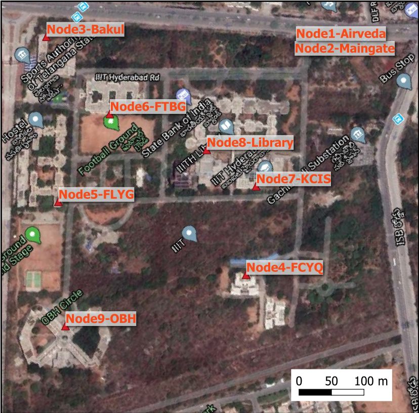
This paper focuses on studying the dense deployment based                 at IIIT-H for stability of the connectors between the sensors
air pollution monitoring using IoT enabled low-cost sensor                   and the microcontroller.
nodes in Indian urban conditions. For this, eight sensor nodes
measuring PM2.5 and PM10 are developed and deployed in
IIIT-H campus, which is 0.267 km2 . A web-based dashboard
                                                                                                                                Thingspeak
is developed to easily monitor the real-time air pollution1 . One
                                                                                       DHT22         NodeMCU
of the eight deployed nodes is co-located with commercially                                                                          LAN or 4G
available and factory-calibrated sensor node with a view of
calibrating developed sensor nodes. The data is collected from                         SDS011         ESP8266                    Access
these nine nodes for approximately five months. Correlation                                                                      Point
                                                                                                                      WiFi
analysis is done to understand correlation between different                                Sensor Node
nodes in this denser (than traditional) deployment. For spatial
                                                                                                       (a) Block architecture
interpolation, inverse distance weighing (IDW) scheme is used
on these nodes for the data collected before and during the
bursting of firecrackers on the main night of Diwali (one of
the most popular festivals in India) to show the variability
pattern in a small campus, hot spot detection and need for a
dense deployment to provide better local pollution indicators.
   The paper is organized as follows. In Section II, details on
IoT network development and deployment along with mea-
surement campaign are presented followed by data analysis
tools in III. Section IV present the results while Section V                                            (b) Circuit diagram
concludes the paper.
                                                                             Fig. 1. Block and circuit diagrams of sensor node developed at IIIT-H for
      II. I OT N ETWORK I MPLEMENTATION AND F IELD                           monitoring PM values.
                     M EASUREMENTS
A. Sensor Node Implementation                                                                             TABLE I
   Figs. 1(a) and 1(b) show the block architecture and circuit                S PECIFICATIONS OF SENSORS USED IN THE DEVELOPED SENSOR NODE .
diagram, respectively, of the PM monitoring sensor node                       Sensor               Parameter          Resolution     Relative error
developed at IIIT-H. Each node consists of ESP8266 based                      SDS011 [10]          PM2.5, PM10        0.3µg m−3      Max. of ±15%,
NodeMCU microcontroller and sensors for PM, temperature                                                                              ±10 µg m−3
and humidity. The specifications of the sensors used are                      DHT22 [11]           Temperature        0.1◦C          ±0.5◦C
                                                                              DHT22 [11]           Humidity           0.1%           ±2%
given in Table I. Nova PM SDS011 which is light scattering
principle based sensor, has been used for PM2.5 and PM10
measurements as it has been shown to have best performance                      Fig. 2 shows a deployment ready sensor node which consists
among several low cost PM sensors in terms of closeness to                   of sensors, a NodeMCU, a 5000 mA h power bank, 4G based
the expensive and accurate beta attenuation mass (BAM) and                   portable WiFi routers (VoLTE-based JioFi JMR1040 [12]) and
reproducibility among different SDS011 units [7]. Since the                  a weather shield. Power bank is needed for power backup
light scattering based PM sensors do not perform reliably at                 in case of any fluctuations or drop in the power supply.
extreme temperature and humidity conditions, DHT22 is used                   A weather shield design with vents shown is used along
to monitor these parameters for reliability of SDS011 sensor                 to cater the ambient air flow requirements of DHT22 for
readings.                                                                    temperature and humidity. The components are enclosed in
   NodeMCU samples data from the sensors and transmits it                    a poly carbonate box of IP65 rating as the deployment is
periodically via WiFi to ThingSpeak [9], which is a cloud                    outdoors. IP65 enclosures offer complete protection against
based IoT platform for storing and processing data using                     dust particles and a good level of protection against water. 4G
MATLAB, for logging the data. NodeMCU uses on-chip                           based WiFi router shown in the figure is not common to all the
ESP8266 module to connect to available WiFi access point for                 nodes deployed and is used only when the node is deployed
internet connection. NodeMCU samples the Nova PM SDS011                      outside campus WiFi coverage.
sensor for PM2.5 and PM10 in µg m−3 and DHT22 sensor for                     B. IoT Network Deployment
environmental conditions temperature and relative humidity in
◦                                                                               The prototype deployment and measurement region is the
  C and % respectively at a sampling rate of 15 seconds and the
                                                                             IIIT-H campus, Gachibowli, Hyderabad, India as shown in
network delay added for the communication with the server.
                                                                             Fig.3. The area of the measurement region is 66 acres (0.267
The connections are made using a PCB printed and designed
                                                                             km2 ). In this small campus, eight nodes developed at IIIT-
 1 The website is live but the historic data, schematics and codes will be   H were deployed outdoors at locations shown in Fig. 3. The
made public once the paper is published.                                     figure also shows the notations and numbering of the nodes,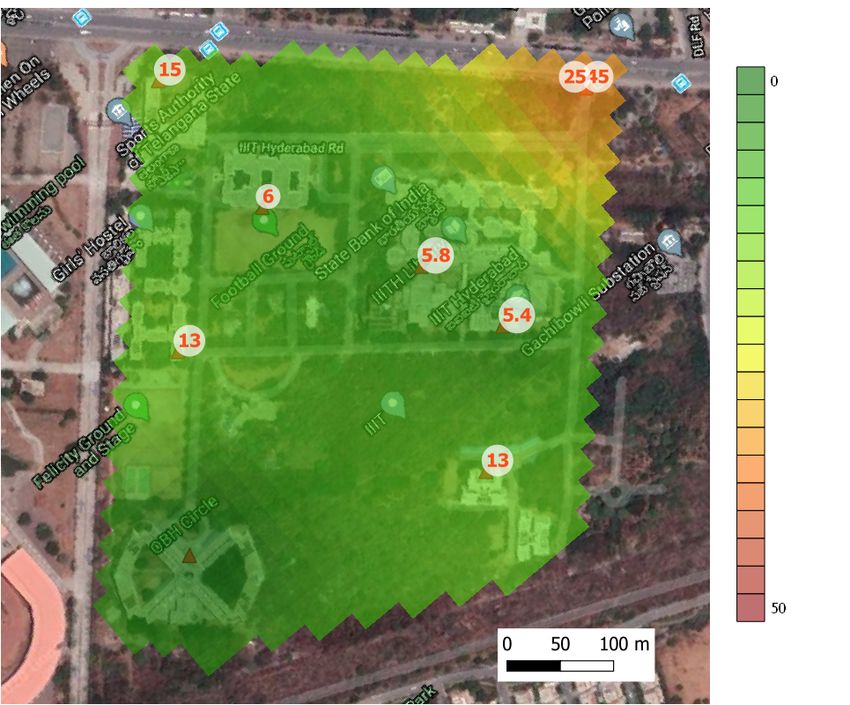
with Node2-MainGate as shown in Fig. 3.
                                                                     All the nodes are connected to continuous power supply.
                                                                  Nodes 4,6 and 8 are connected to the WiFi provided by the
                                                                  access points which are part of the campus WiFi network.
                                                                  Node 7 could connect to the campus WiFi network but with
                                                                  weak signal strength, which sometimes resulted in connection
                                                                  outages and data loss. To avoid this and strengthen the WiFi
                                                                  signal, a NodeMCU has been deployed in appropriate location
                                                                  as a WiFi repeater. Nodes 2,3,5 and 9 are out of the campus
                                                                  WiFi coverage and have been equipped with individual 4G
                                                                  based portable JioFi WiFi routers for internet connectivity.
                                                                  Node1-Airveda is using WiFi provided by JioFi connected to
                                                                  Node2-MainGate since these two nodes are collocated.
                                                                     Each of the eight IIIT nodes (i.e., nodes 2 to 9) uploads
                                                                  the sampled sensor data, namely PM2.5, PM10, temperature
                                                                  and relative humidity to individual channels created on the
                                                                  ThingSpeak server using GET method of the HTTP protocol.
                                                                  Node1-Airveda uses ESP8266 for WiFi communication and
                Fig. 2. Outdoor air pollution node.               uploads data to Airveda server. The same data is retrieved
                                                                  using Airveda application program interface (API) and saved
                                                                  in a separate channel in the ThingSpeak server.
                                                                  C. Development of web-based dashboard

                                                                                                    Front-End
                                                                                                                    HTML
                                                                                                                    code

                                                                             Map Data
                                                                           OpenStreetMap
                                                                                                                    Leaflet

                                                                                                                  JavaScript

                                                                                                                     AJAX
                                                                              ThingSpeak
                                                                               Rest API
                                                                                                                  Back-End

                                                                  Fig. 4. Process flow of website development for real-time PM monitoring.

                                                                     The website developed for displaying the real-time PM
                                                                  values is hosted at the address https:/spcrc.iiit.ac.in/air/. Fig.
                                                                  4 shows the process flow of the web-bas. The webpage is
            Fig. 3. Sensor deployment in IIIT-H campus            designed such that the data is fetched from the ThingSpeak
                                                                  server and is displayed on the webpage on an open source map
                                                                  OpenStreetMap [14]. The front-end of the webpage is designed
which will be followed for the rest of the paper. Before          in hyper text markup language (HTML) and back-end is
deploying, these eight nodes were collocated in a lab and         designed in Javascript. To get the map data, we used Javascript
measured data for seven days to ensure that none of the devices   library Leaflet [15]. To get data from ThingSpeak, another
is too deviant from the bunch. The deployment period of the       Javascript library asynchronous Javascript and XML (AJAX)
nodes has been from 26 October 2019 to 10 April 2020 (more        is used, which allows us to get data from the ThingSpeak
than 5 months).                                                   API using the GET function. After we get the data from
   In addition to the eight nodes, a ninth node was also de-      the ThingSpeak API, the data is averaged and a colour is
ployed by buying off-the-shelf commercial node from Airveda       associated with the data value. Next, using Leaflet functions,
[13]. This node was factory calibrated with respect to BAM        the marker colour and information on the map is set. The
and has been used as a reference node for our nodes in this       process then goes to sleep. The complete process is repeated
work. This node is denoted as Node1-Airveda and is collocated     every 5 minutes. Note that this dashboard does not show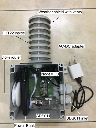
Node1-Airveda at the moment as it can be viewed on the               this paper. Kendall’s tau (τ ), which is a non-parametric rank-
Airveda webpage or app by adding the station ID.                     based measure of dependence is defined as
             III. DATA P ROCESSING M ETHODS                                                       nc − nd
                                                                                             τ=           ,
A. Data Cleaning and Preprocessing                                                                nc + nd
   The following tasks were done to convert the raw data
                                                                     where nc and nd are the numbers of concordant pairs and
received from the sensor nodes into a usable data set:
                                                                     discordant pairs respectively. For a given pair (xi , yi ) and
   • It is essential to remove the outliers in a raw dataset
                                                                     (xj , yj ), let us define z = (xi − xj )(yi − yj ). This pair is
     as there are few extreme values that deviate from other         concordant if z > 0 and discordant if z < 0.
     samples in the data, which might be a result of several
                                                                        3) Spatial Interpolation: It is not practical to deploy and
     factors. Data cleaning can be done using clustering based
                                                                     measure PM values at every location in the area of interest.
     outlier detection, which is a well known unsupervised
                                                                     However, using nearest measurement point to approximate the
     method used extensively. In this paper, density based clus-
                                                                     PM value at a location of interest may lead to erroneous
     tering algorithm in [16] has been employed to identify the
                                                                     results given the variability of pollution levels and weather
     outliers and the vectors with outlier have been dropped.
                                                                     in different locations in an urban environment. This can be
     Environmental conditions such as temperature and hu-
                                                                     mitigated by using spatial interpolation to estimate the PM
     midity can affect the working of laser based PM sensors
                                                                     values at unmeasured locations using known values at the
     like SDS011. For example, there is overestimation of PM
                                                                     measurement locations. In this paper, we have used IDW,
     values at higher humidity. As such, these points also act
                                                                     which is one of the simplest and popular deterministic spatial
     as outliers and the corresponding vectors are removed
                                                                     interpolation technique [17]. IDW follows the principle that
     using the density based clustering.
                                                                     the nodes that are closer to the location of estimation will
   • Data averaging helps to look past random fluctuation and
                                                                     have more impact than the ones which are farther away. IDW
     see the central trend of a data set. The sensor used in
                                                                     uses linearly weighted combination of the measured values at
     the PM measurements has a relative error of 15% so
                                                                     the nodes to estimate the parameter at the location of interest.
     averaging the data helps to smooth the time series curve.
                                                                     The weight corresponding to a node is a function of inverse
B. Analysis tools                                                    distance between the location of the node and the location of
   1) Quantile-Quantile plots: The quantile-quantile plot or         the estimate. In this paper, weights have been chosen to be
QQ plot is an analysis tool to assess if a pair of data variables’   inverse distance squared.
population possibly came from same distribution or not. A QQ
plot is a scatterplot created by plotting two sets of quantiles                      IV. A NALYSIS AND R ESULTS
against one another. If both sets of quantiles have come from
the same distribution, the scatter plot form a line that’s roughly      The following analyses were applied on the obtained data
straight. Many distributional aspects like shifts in location,       set after cleaning and preprocessing: QQ plots, time series
scale, symmetry, and the presence of outliers can be detected        plots, correlation analysis and spatial analysis.
from these plots. For two data sets that come from similar
populations whose data distribution functions differ only by         A. Quantile-quantile plots (QQplots)
shifts mentioned earlier, the data points lie along a straight
line displaced either up or down from the 45-degree reference           QQ plots have been used on the two co-located nodes
line. QQ plots help us understand the distributional features of     Node1-Airveda and Node2-Maingate to verify the distribution
the data sets and provide necessary confidence for assumptions       similarity. Node1-Airveda is an air quality monitoring device
for further analysis.                                                from Airveda which has been tested against the standard PM
   2) Correlation Analysis: Correlation is a bivariate analysis      sensor BAM monitor and Node2-Maingate is the sensor node
that measures the strength of association between two vari-          developed at IIIT-H. QQplots have been plotted with one-hour
ables and the direction of the relationship. The correlation         averaged data for PM2.5 in Fig. 5(a) and for PM10 in Fig. 5(b)
coefficient is a statistic tool used to measure the extent of        with Node1-Airveda on horizontal axis and Node2-Maingate
the relationship between variables when compared in pairs.           on the vertical axis. The plots show linearity for most part
In terms of the strength of the relationship, the value of the       with most of the sample points close to straight line with
correlation coefficient varies between +1 and -1. There are          high density and very few points deviating from the linear
several types of correlation coefficients such as Pearson and        relationship for both PM2.5 and PM10 samples. In the case
Kendall. Pearson’s correlation is one of the most commonly           of PM2.5 few deviating points belong to the higher end of the
used correlation coefficient but makes several assumptions on        distribution while in the case of PM10 samples, few deviations
the data such as normally distributed variables, linearly related    can be seen at both lower and higher ends of the distribution.
variables, complete absence of outliers and homoscedasticity.        From the plots, it is safe to assume that the populations of the
On the other hand, Kendall’s tau doesn’t require the above           data samples of Node1-Airveda and Node2-Maingate follow
mentioned assumptions and is more suitable for the work in           a similar distribution with very few samples deviating.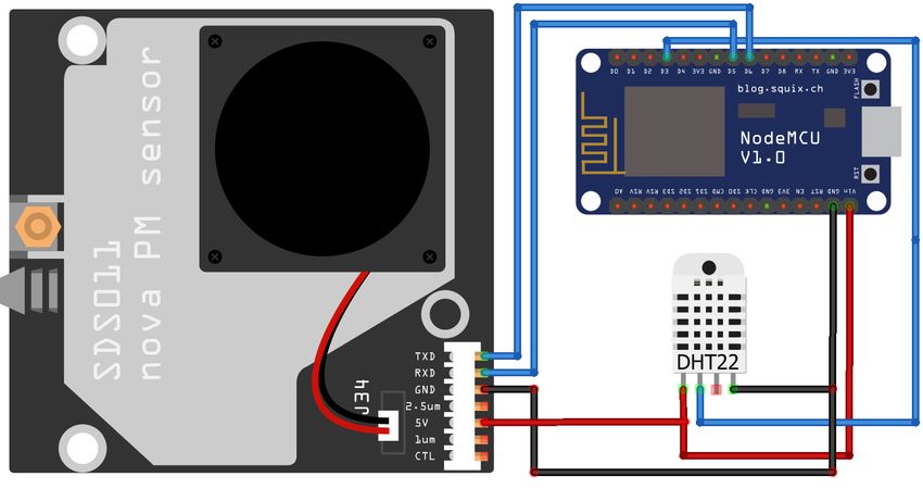
(a) PM 2.5                                                           (b) PM 10

Fig. 5. QQ plots for PM2.5 and PM10 between co-located nodes at the main gate, i.e., Node1-Airveda and Node2-Maingate.

                                                      (a) PM2.5

                                                      (b) PM10

                            Fig. 6. Time Series of PM2.5 and PM10 values (daily averages).
B. Time series plots for PM2.5 and PM10 of PM2.5 and PM10 samples. The values of the Kendall’s
Fig. 6 shows time series plots for nine nodes with daily coefficients are shown in the Fig. 7. The Kendall’s coefficient
averaging for both PM2.5 and PM10 samples. The deployment varies from a value of 0.1538 to 0.9492 for PM2.5 samples and
period of the nodes has been more than five months from 26 0.14598 to 0.8954 for PM10 samples. The significant variation
October 2019 to 10 April 2020. Four important observations between correlation values highlight the spatial variability
can be made from this figure. First, a clear peak can be between the PM values at different nodes. The maximum
observed for all nodes on 27 October 2019 resulting from amount of correlation has been shown by the Node6-FTBG
the widespread burning of firecrackers during the celebration and Node8-Library. The least correlation for both PM2.5 and
of Diwali festival. Dominant peaks can be seen at Node5- PM10 is shown by Node2-Maingate and Node9-OBH, which
FLYG and Node4-FCYQ, where residents of the campus burst are farthest from each other by about 600 m. Node5-FLYG and
crackers. However, the peak in PM values due to fire-crackers Node6-FTBG also show very high amount of correlation of
died down in next few days. Second observation from the 0.9223 and 0.8926 for PM2.5 and PM10 values, respectively.
figure is that the PM values again started increasing with the Node5-FLYG and Node6-FTBG both are placed in similar
onset of winter in November 2019 and peak in December geographical conditions (facing an open ground). Node9-OBH
2019 and January 2020 during peak winter with temperatures shows very less correlation in most of the pairs of nodes, as the
in Hyderabad between 10-30 ◦C. Third observation is that node is located far inside the residential block of the campus
as the winter weakens in February 2020, the PM values in with close to zero vehicle frequency.
general started decreasing. Final observation is that the PM Kendall’s coefficients have also been calculated between the
plots show very low values of PM in March and April 2020. Node1-Airveda and the six CPCB stations deployed across the
This can be attributed to the drastic reduction in traffic and city and the values are shown in the Table II. The kendall’s
construction activities in and around campus as the State and coeffiecients vary from as low as 0.17 to maximum being 0.68
Central Government gradually started increasing restrictions to in the case of PM2.5 and 0.37 to 0.47 in the case of PM10. In
prevent spread of Covid-19 from the first week of March and general the values are lesser than 0.5 which implies very weak
finally declared nationwide lockdown since 22 March 2020 till relationship between the stations. The nearest CPCB station
30 April 2020. from the Node1-Airveda show Kendall tau values of 0.47 and
0.68 for PM10 and PM2.5 respectively indicating the very low
C. Correlation Analysis relation between two locations which are approximately only
3 km apart. This shows the necessity for local PM monitoring
for a better understanding of the street-level values.
TABLE II
K ENDALL’ S COEFFICIENTS OF CORRELATION BETWEEN N ODE 1-A IRVEDA
AND CPCB STATIONS .
Node1-Airveda Kendall’s Coefficients with CPCB stations
PM2.5 0.68 0.59 0.64 0.58 0.17 0.50
PM10 0.47 0.37 0.47 0.42 NA 0.37
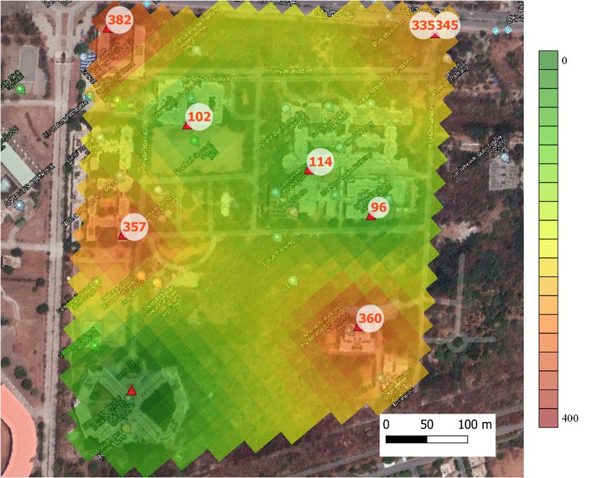
D. Spatial Interpolation
(a) PM 2.5 Figs. 8(a) and 8(b) show IDW based interpolation maps
for PM10 plotted at timestamps 19:00:00 (before burning
crackers) and 22:40:00 (after burning crackers) on the day
of Diwali. In Fig. 8(a), the hot-spot of the PM10 values is
at the Node1-Airveda and Node2-Maingate which are placed
near a six-lane highway and exposed directly to vehicular
pollution. Spatial variation can be clearly seen in Fig. 8(a)
between the nine points in an area of only 66 acres (0.267
km2) with Node6-FTBG, Node7-KCIS and Node8-Library
showing comparatively lower values being in the center of
the campus. In Fig. 8(b), which shows the values at 22:40
after bursting of crackers, the values increase dramatically by
(b) PM 10
10 to 25 times. Now the number of hot-spots has increased to
Fig. 7. Kendall’s correlation between the nodes for PM2.5 and PM10. four, of which Node5-FLYG and Node4-FCYQ are the sites
for bursting crackers while Node1-Airveda, Node2-Maingate
Kendall’s correlation coefficients τ between the nine sen- and Node3-Bakul are affected by both vehicular pollution and
sor nodes have been calculated using five minute averages crackers burned outside the campus. Node9-OBH was off dueof more than five months clearly show significant increase in
PM values during Diwali as well as the noticeable reduction in
PM values during national lockdown during COVID-19. It has
been shown that correlation coefficient between some nodes
in the same campus have low values demonstrating that the
PM values across a small region may be significantly different.
Moreover, the IDW-based spatial interpolation results on the
day of Diwali show significant spatial variation in PM values
in the campus ranging from 96 to 382 for locations just a few
hundred meters apart for PM10. The results also show notable
temporal variations with PM values rising up to 25 times at
the same spot in few hours. Thus, there is sufficient motivation
to use dense deployment of IoT nodes for improved spatio-
temporal monitoring of PM values.
(a) At 17:00
R EFERENCES
[1] P. Landrigan et al., “The Lancet Commission on Pollution and Health,”
Lancet, vol. 391, pp. 464–512, 2018.
[2] M. Tagle et al., “Field performance of a low-cost sensor in the
monitoring of particulate matter in Santiago, Chile,” Environmental
Monitoring and Assessment, vol. 192, no. 171, pp. 18, Feb. 2020.
[3] P. Pant et al., “Monitoring particulate matter in India: Recent trends and
future outlook,” The Verge, vol. 12, no. 1, pp. 45–58, Jan. 2019.
[4] X. Wu, R. Nethery, B. Sabath, D. Braun, and F. Dominici, “Exposure to
air pollution and COVID-19 mortality in the United States,” medRxiv,
Apr. 2020.
[5] National Air Quality Index, accessed 11 Apr. 2020, https://app.cpcbccr.
com/AQI India/.
[6] S. Brienza et al., “A Low Cost Sensing System for Coopertaive Air
Quality Monitoring in Urban Areas,” Sensors, vol. 15, pp. 12242–12259,
2015.
[7] M. Badura, P. Batog, A. Drzeniecka-Osiadacz, and P. Modzel, “Evalu-
ation of Low-Cost Sensors for Ambient PM2.5 Monitoring,” Journal of
Sensors, vol. 2018, no. 5096540, pp. 1–16, 2018.
[8] S. Johnston et al., “City Scale Particulate Matter Monitoring Using
(b) At 22:40 LoRaWAN Based Air Quality IoT Devices,” Sensors, 01 2019.
[9] ThingSpeak, accessed 01 Apr. 2020, https://thingspeak.com/.
Fig. 8. Spatial interpolation of PM10 values in IIIT-H campus using IDW at [10] SDS011 Nova Sensor Specifications, accessed 15 Mar. 2020, http://www.
17:00 hrs and 22:40 hrs on the day of Diwali (27 October 2019). Note the inovafitness.com/en/a/chanpinzhongxin/95.html.
difference in scales in the two maps for convenient viewing. [11] DHT22 Sensor Specifications, accessed 15 Mar. 2020, http://www.
adafruit.com/datasheets/DHT22.pdf.
[12] JioFi Portable Router JMR1040, accessed 21 Jan. 2020, https://www.
to some technical issue on the evening of Diwali, which has jio.com/shop/en-in/router-jmr1040-white-/p/491193523.
[13] Airveda Outdoor Air Quality Monitor, accessed 01 Apr. 2020, https:
affected the interpolated values at that point and resulting in //www.airveda.com/outdoor-air-quality-monitor.
lower values than the actual. Fig. 8(b) shows three nodes and [14] OpenStreetMap, accessed 03 Mar. 2020, https://www.openstreetmap.
the area in the center of the campus which are surrounded org/.
[15] Leaflet- A Javascript library for mobile-friendly interactive maps, ac-
by the pollution hot-spots but yet show significantly lower cessed 01 Feb. 2020, https://leafletjs.com/.
values of PM. The spatial variation within the nine nodes is [16] M. Çelik, F. Dadaşer-Çelik, and A. Ş. Dokuz, “Anomaly detection
dominantly seen and hence demonstrates the need for local in temperature data using DBSCAN algorithm,” in International
Symposium on Innovations in Intelligent Systems and Applications, 2011,
deployment of sensor nodes for accurate monitoring of the pp. 91–95.
air quality conditions locally. Fig. 8 also show the temporal [17] P. Burrough and R. McDonnell, Principles of Geographical Information
variation of the values within a small time period of five hours Systems, Oxford University Press, 1998.
an increase in value from 13 to around 360 at the Node5-
FLYG and Node4-FCYQ. Although similar results have been
obtained for PM2.5, they are not shown here for brevity.
V. C ONCLUSION
In this paper, the dense deployment of IoT nodes has been
evaluated for monitoring PM values in urban Indian setting.
For this, nine nodes have been deployed in a small campus of
IIIT-H. A web-based dashboard has been developed for real
time PM monitoring. The measurements done over the periodYou can also read