Audiogmenter: a MATLAB toolbox for audio data augmentation
←
→
Page content transcription
If your browser does not render page correctly, please read the page content below
The current issue and full text archive of this journal is available on Emerald Insight at:
                         https://www.emerald.com/insight/2210-8327.htm

Audiogmenter: a MATLAB toolbox                                                                                          A MATLAB
                                                                                                                         toolbox for
  for audio data augmentation                                                                                             audio data
                                                                                                                       augmentation
                                         Gianluca Maguolo
                                 University of Padua, Padua, Italy
                                         Michelangelo Paci
                          Tampere University, Tampere, Finland, and                                                    Received 25 March 2021
                            Loris Nanni and Ludovico Bonan                                                               Revised 18 April 2021
                                                                                                                        Accepted 18 April 2021
                                 University of Padua, Padua, Italy

Abstract
Purpose – Create and share a MATLAB library that performs data augmentation algorithms for audio data.
This study aims to help machine learning researchers to improve their models using the algorithms proposed
by the authors.
Design/methodology/approach – The authors structured our library into methods to augment raw audio
data and spectrograms. In the paper, the authors describe the structure of the library and give a brief
explanation of how every function works. The authors then perform experiments to show that the library is
effective.
Findings – The authors prove that the library is efficient using a competitive dataset. The authors try multiple
data augmentation approaches proposed by them and show that they improve the performance.
Originality/value – A MATLAB library specifically designed for data augmentation was not available
before. The authors are the first to provide an efficient and parallel implementation of a large number of
algorithms.
Keywords Audio augmentation, Data augmentation, Audio classification, Spectrogram, Convolutional neural
network
Paper type Research paper

1. Introduction
Deep neural networks achieved state of the art performances in many artificial intelligence
fields, such as image classification [1], object detection [2] and audio classification [3].
However, they usually need a very large amount of labeled data to obtain good results and
these data might not be available due to high labeling costs or due to the scarcity of the
samples. Data augmentation is a powerful tool to improve the performance of neural
networks. It consists in modifying the original samples to create new ones, without changing
their labels [4]. This leads to a much larger training set and, hence, to better results. Since data
augmentation is a standard technique that is used in most papers, a user-friendly library
containing efficient implementations of these algorithms would be very helpful to
researchers.

© Gianluca Maguolo, Michelangelo Paci, Loris Nanni and Ludovico Bonan. Published in Applied
Computing and Informatics. Published by Emerald Publishing Limited. This article is published under
the Creative Commons Attribution (CC BY 4.0) licence. Anyone may reproduce, distribute, translate and
create derivative works of this article (for both commercial and non-commercial purposes), subject to full
attribution to the original publication and authors. The full terms of this licence may be seen at http://
creativecommons.org/licences/by/4.0/legalcode
    The authors thank three anonymous reviewers for their constructive comments and for their                               Applied Computing and
                                                                                                                                         Informatics
comments on an earlier version of this manuscript. The authors are also thankful to the experts who                     Emerald Publishing Limited
provided valuable suggestions on the version of this paper presented at the website: https://arxiv.org/                            e-ISSN: 2210-8327
                                                                                                                                  p-ISSN: 2634-1964
ftp/arxiv/papers/1912/1912.05472.pdf [32].                                                                             DOI 10.1108/ACI-03-2021-0064
ACI In this paper we introduce Audiogmenter, a MATLAB toolbox for audio data
augmentation. In the field of audio classification and speech recognition, to the best of our
knowledge, this is the first library specifically designed for audio data augmentation. Audio
data augmentation techniques fall into two different categories, depending on whether they
are directly applied to the audio signal [5] or to a spectrogram generated from the audio signal
[6]. We propose 15 algorithms to augment raw audio data and 8 methods to augment
spectrogram data. We also provide the functions to map raw audios into spectrograms. The
augmentation techniques range from very standard techniques, like pitch shift or time delay,
to more recent and very effective tools like frequency masking. The library is available at
https://github.com/LorisNanni/Audiogmenter. The main contribution of this paper is to share
a set of powerful data augmentation tools for researchers in the field of audio-related artificial
intelligence tasks.
The rest of the paper is organized as follows. Section 2 describes the specific problem
background and our strategy for audio data augmentation. Section 3 details the
implementation of the toolbox. Section 4 provides one illustrative example. Section 5
contains experimental results. In Section 6, conclusions are drawn.
2. Related work
To the best of our knowledge, Audiogmenter is the first MATLAB library specifically
designed for audio data augmentation. Such libraries exist in other languages like Python. A
well-known Python audio library is Librosa [7]. The aim of Librosa was to create a set of tools
to mine audio databases, but the result was an even more comprehensive library useful in all
audio fields. Another Python library is Musical Data Augmentation (MUDA) [8], which is
specifically designed for audio data augmentation and is not suitable for more general audio-
related tasks. MUDA only contains algorithms for pitch deformations, time stretching and
signal perturbation but does not contain algorithms like pass filters that would not be useful
for generating music data.
Some audio augmentation toolboxes are also available in MATLAB. A famous library is
the time-scale modification (TSM) toolbox. It contains the MATLAB implementations of
many TSM algorithms [9, 10]. TSM algorithms allow to modify the speed of an audio signal
without changing its pitch. They provide many algorithms to do that because it is not trivial
to do while maintaining the audio plausible, and every algorithm addresses the problem in a
different way. It is clear that this toolbox can be used only on those audio tasks that do not
heavily depend on the speed of the sounds.
Recently, the 2019b version of MATLAB included a built-in audio data augmenter for
training neural networks. It contains very basic functions which have the advantage of being
computed on every mini-batch during training; hence, they do not use a large quantity of
memory. However, they can only be applied to the input layers of recurrent networks.
On first approximation, an audio sample can be represented as an M by N matrix, where M
is the number of samples acquired at a specific frame rate (e.g. 44100 Hz), and N is the number
of channels (e.g. one for mono and more for stereo samples). Classical methods for audio
classification consisted in extracting acoustic features, e.g. Linear Prediction Cepstral
Coefficient or Mel-Frequency Cepstral Coefficients, to build feature vectors used for training
Support Vector Machines or Hidden Markov Models [11]. Nevertheless, with the diffusion of
deep learning and the growing availability of powerful Graphic Processing Units (GPUs), the
attention moved toward the visual representations of audio signals. They can be mapped into
spectrograms, i.e. graphical representations of sounds as functions of time and frequency,
and then classified using Convolutional Neural Networks (CNN) [12]. Unfortunately, several
audio datasets (especially in the field of animal sound classification) are limited, e.g. CAT
sound dataset (2965 samples in 10 classes) [13], BIRD sound dataset (2762 samples in 11classes) [14], marine animal sound dataset (1700 samples in 32 classes) [15] etc. Neural A MATLAB
networks are prone to overfitting; hence, data augmentation can strongly improve their toolbox for
performance.
Among the techniques used in the literature to augment raw audio signals, pitch shift,
audio data
noise addition, volume gain, time stretch, time shift and dynamic range compression are the augmentation
most common. Moreover, the Audio Degradation Toolbox (ADT) provides further techniques
such as clipping, harmonic distortion, pass filters, MP3 compression and wow resampling
[16]. Furthermore, Sprengel et al. [5] showed the efficacy of augmentation by summing two
different audio signals from the same class into a new signal. For example, if two samples
contain tweets from the same bird species, their sum will generate a third signal still
belonging to the same tweet class. Not only the raw audio signals but also their spectrograms
can be augmented using standard techniques [6], e.g. time shift, pitch shift, noise addition,
vocal tract length normalization (VTLN) [17], equalized mixture data augmentation (EMDA)
[18], frequency masking [19] and thin-plate spline warping (TPSW) [20].
3. Background and strategy
Given an audio dataset X with M classes and variable number of samples per class
X ¼ fx1;1 ; . . . xn1 ;1; x1;2 ; . . . xn2 ;2; . . . ; x1;M ; . . . xnM ;M g, where xi;j represents a generic
audio sample i from the class j, we propose to augment xi;j with techniques working on raw
audio signals and to augment the spectrogram Sðxi;j Þ produced by the same raw audio
signals.
In Figure 1, the upper branch shows how, from the original i-th audio sample xi;j from the
class j, we obtain H augmented audio samples AugAh ðxi;j Þ to be converted into the
augmented “Spectrograms from Audio” AugSAh ðxi;j Þ. The lower branch shows how K
augmented “Spectrograms from Spectrogram” AugSSk ðxi;j Þ can be obtained from the
spectrogram of the original audio sample Sðxi;j Þ.
In our tool, we used the function sgram included in the large time-frequency analysis
toolbox (LTFAT) [21] to convert raw audios into spectrograms.
Figure 1 depicts our strategy; from the original audio sample xi;j we obtain H intermediate
augmented audio samples AugAh ðxi;j Þ that are then converted into the “Spectrograms from
Audio” AugSAh ðxi;j Þ; from the original spectrogram Sðxi;j Þ we obtain K augmented
“Spectrograms from Spectrogram” AugSSk ðxi;j Þ. The H þ K augmented spectrograms can
then be used to train a CNN. In case of limited memory availability, one CNN can be trained
Figure 1.
Augmentation
strategy implemented
in AudiogmenterACI with the H AugSA spectrograms, another with the K AugSS spectrograms and finally the
scores can be combined by a fusion rule.
4. Toolbox structure and software implementation
Audiogmenter is implemented as a MATLAB toolbox, using MATLAB 2019b. We also
provide an online help as documentation (in the ./docs/folder) that can be integrated into the
MATLAB Help Browser just by adding the toolbox main folder to the MATLAB path.
The functions for the augmentation techniques working on raw audio samples are
included in the folder ./tools/audio/. In addition to our implementations of methods such as
applyDynamicRangeCompressor.m and applyPitchShift.m, we also included four toolboxes,
namely the ADT by Mauch et al. [16], LTFAT [21], the Phase Vocoder from www.ee.columbia.
edu/∼dpwe/resources/matlab/pvoc/and the Auditory Toolbox [22].
The functions for the augmentation methods working on spectrograms are grouped in the
folder ./tools/images/. In addition to our implementations of methods such as noiseS.m,
spectrogramShift.m, spectrogramEMDA.m etc., we included and exploited also a modified
version of the code of TPSW [20].
Every augmentation method is contained in a different function. In ./tools/, we also
included the wrappers CreateDataAUGFromAudio.m and CreateDataAUGFromImage.m,
using our augmentation techniques, respectively, from raw audio and spectrograms with
standard parameters.
We now describe the augmentations and provide some suggestions on how to use them in
the correct applications:
(1) applyWowResampling [16] is similar to pitch shift, but the intensity changes along
time. The signal x is mapped into:
sinð2π fm xÞ
FðxÞ ¼ x þ am
2 π fm
where x is the input signal, and am ; fm are parameters. This algorithm depends on the
Degradation Toolbox. This is a very useful tool for many audio task and we recommend
its use, although we suggest to avoid it for task that involves music, since changing the
pitch with different intensities over time might lead to unnatural samples.
(2) addNoise adds white noise to the input signal. It depends on the Degradation
Toolbox. This algorithm improves the robustness of a tool by improving its
performance on noisy signals; however, this improvement might be unnoticed when
the test set is not noisy. Besides, for tasks like sound generation one might want to
avoid a neural network to learn from noise data.
(3) applyClipping normalizes the audio signal leaving a percentage X of the signal
outside the interval [1, 1]. Those parts of the signal are then mapped to sign(x).
This algorithm depends on the Degradation Toolbox. Clipping is a common
technique in audio processing; hence, many recorded or generated audio might be
played by a mobile device after having been clipped. If the tool the reader wants to
train must recognize this kind of signal, we recommend this augmentation.
(4) applySpeedUp modifies the speed of the signal by a given percentage. This algorithm
depends on the Degradation Toolbox. We suggest to use this augmentation when
the speed of a signal is not an important property of the signal.
(5) HarmonicDistortion [16] applies the sine function to the signal multiple times. This
algorithm depends on the Degradation Toolbox. This is a very specificaugmentation that is not suitable for most applications. It is very useful to augment A MATLAB
the input signals when the objective of the reader is working with sounds generated toolbox for
by electronic devices, since they might apply a small harmonic distortion to the
original signal.
audio data
augmentation
(6) applyGain increases the gain of the input signal. We always recommend to use this
algorithm, in general it can always be useful.
(7) applyRandTimeShift randomly takes a signal xðtÞ as input, where 0 ≤ t ≤ T. Then a
random time t * is sampled and the new signal is yðtÞ ¼ xðmodðt þ t * ; TÞÞ. In words,
the first and the second part of the file are randomly switched. This algorithm is very
useful, but do not use it if the order of the events in the input signals that you are
working with is important. For example, it is not good for speech recognition. It is
useful for tasks like sound classification.
(8) applySoundMix [23] sums two audio signals from the same class. This algorithm
depends on the Degradation Toolbox. We suggest to use this algorithm often. In
particular, it is useful for multi-label classification or for tasks that involve multiple
audio sources at the same time. It is worth noticing that is has also been used for
single-label classification [24].
(9) applyDynamicRangeCompressor applies, as its name says, dynamic range
compression [25]. This algorithm modifies the frequencies of the input signal. We
refer to the original paper for a detailed description. Dynamic range compression is
used to preprocess the audio before being played by an electronic device. Hence, a
tool that deals with this kind of sounds should include this algorithm in its
augmentation strategy.
(10) appltPitchShift increases or decreases the frequencies of an audio file. This is one of
the most common augmentation techniques. This algorithm depends on Phase
Vocoder.
(11) applyAliasing resamples the audio signal with a different frequency. It violates the
Nyquist-Shannon sampling theorem on purpose [26] to degradate the audio signal.
This is a modification of the sound that might occur when unsafely changing its
frequency. This algorithm depends on the Degradation Toolbox. In general, it does
not provide great improvement for machine learning tasks. We include it in our
toolbox because it might be useful to reproduce the error due to the oversampling of
low sampled signals, although they are quite rare in audio applications.
(12) applyDelay adds a sequence of zeros at the beginning of the signal. This algorithm
depends on the Degradation Toolbox. This time delay might be useful in any
situation. In particular, we suggest to use it when the random shift of point 7 is not
appropriate.
(13) applyLowpassFilter attenuates the frequencies above a given threshold f1 and blocks
all the frequencies above a given threshold f2. This algorithm depends on the
Degradation Toolbox. Low pass filters are useful when high frequencies are not
relevant for the audio task.
(14) applyHighpassFilter attenuates the frequencies below a given threshold f1 and blocks
all the frequencies below a given threshold f2. This algorithm depends on the
Degradation Toolbox. Low pass filters are useful when high frequencies are not
relevant for the audio task.ACI (15) applyInpulseResponse [16] modifies the audio signal as if it was produced by a
particular source. For example, it simulates the distortion given by the sound system
of a smartphone, or it simulates the echo and the background noise of a great hall.
This algorithm depends on the Degradation Toolbox. This augmentation is very
useful if the reader needs to train a tool that must be robust and work in different
environments.
The functions for spectrogram augmentation are:
(1) applySpectrogramRandomShifts applies pitch and time shift. These augmentations
are always useful.
(2) applySpectrogramSameClassSum [23] sums the spectrograms of two images with the
same label. This is a very useful algorithm. In particular, it is useful for multi-label
classification or for tasks that involve multiple audio sources at the same time. It is
worth noticing that it has also been used for single-label classification [24].
(3) applyVTLN creates a new image by applying VTLN [17]. For a more detailed
description of the algorithm, we refer to the original paper. Since vocal track length is
one of the main inter-speaker differences in speech recognition, VTLN is particularly
suited for this kind of applications.
(4) spectrogramEMDAaugmenter applies EMDA [18]. This function computes the
weighted average of two randomly selected spectrograms belonging to the same
class. It also applies a random time delay to one spectrogram and a perturbation to
both spectrograms, according to the formula
saug ðtÞ ¼ αΦðs1 ðtÞ; ψ 1 Þ þ ð1 αÞΦðs2 ðt βTÞ; ψ 2 Þ
where α; β are two random numbers in ½0; 1, T is the maximum time shift and Φ is an
equalizer function. We refer to the original paper for a more detailed description. This is a
very general algorithm that works in very different situations. It is a more general version
of applySpectrogramSameClassSum.
(5) applySpecRandTimeShift does the same as applyRandTimeShift, but it works for
spectrograms.
(6) randomImageWarp applies Thin-Spline Image Warping [20] (TPS-Warp) to the
spectrogram, on the horizontal axis. TPS-Warp consists in the linear interpolation of
the points of the original image. In practice, it is a speed up where the change in speed
is not constant and has average 1. This function is much slower than the others. It can
be used in any application.
(7) applyFrequencyMasking sets to a constant parameter the value of some rows and
some columns of the spectrogram. The effect is that it masks the real value of the
input for randomly chosen times and frequencies. It was proposed in [3]. It was
successfully used for speech recognition.
(8) applyNoiseS adds noise to the spectrograms by multiplying the value of a given
percentage of the pixels by a random number whose average is one and whose
variance is a parameter. Similarly to applyNoise, this function increases the
robustness of the trained tool on noisy data; however, if the test set is not noisy,
the improvement might be unnoticed.5. Illustrative examples A MATLAB
In the folder ./examples/we included testAugmentation.m that exploits the two wrappers toolbox for
detailed in the previous section to augment six audio samples and their spectrograms, and
plotTestAugmentation.m that shows the results from the previous function. The augmented
audio data
spectrograms can be seen in Figures 2 and 3. augmentation
Figure 2 shows the effect of transforming the audio into a spectrogram and then applying
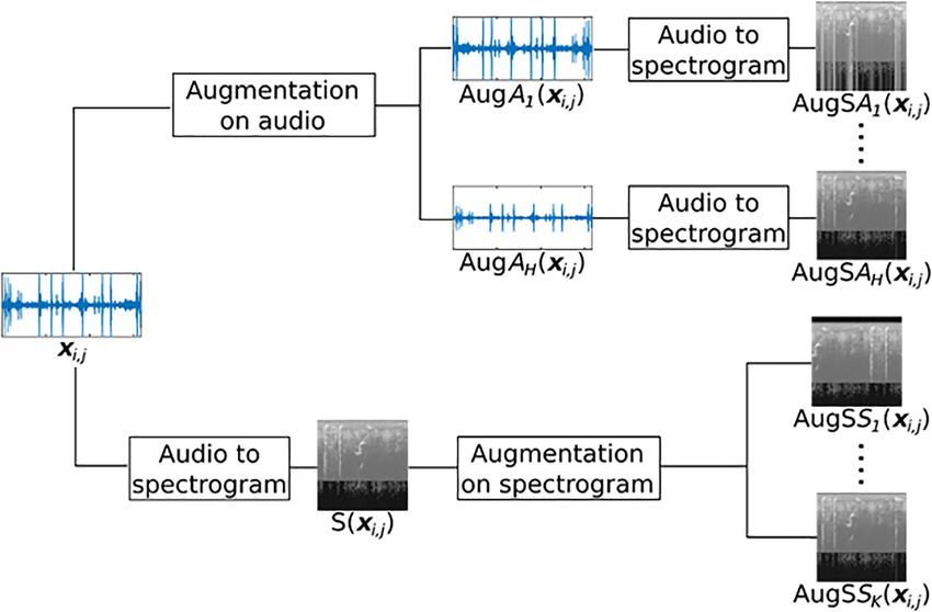
the spectrogram augmentations described in the previous section. Figure 3 shows the
spectrograms obtained by the original and the transformed audio files. Although these
figures are different, it is possible to recognize specific features that are left unchanged by the
augmentation algorithms, as it is desired for this kind of algorithms.
In Figure 2, the top left corner shows the spectrogram from the original audio sample.
Seven techniques were used to augment the original spectrogram. The description of the
outcomes is in the previous section.
In addition, we provide six audio samples from www.xeno-canto.org (original samples
in ./examples/OriginalAudioFiles/and listed as MATLAB table in ./examples/SmallInput
Datasets/inputAugmentationFromAudio.mat) and six spectrograms generated by sgram.m
from the aforementioned audio samples (in ./examples/SmallInputDatasets/inputAugmentation
FromSpectrograms.mat). The precomputed results for all the six audio samples and
spectrograms are provided in the folder ./examples/AugmentedImages/.
In Figure 3, the top left corner shows the spectrogram of the original audio sample. We
used 11 audio augmentation methods and extracted the spectrograms. The description of the
outcomes is in the previous section.
6. Experimental results
The ESC-50 dataset [27] contain 2000 audio samples evenly divided in 50 classes. These
classes are, for example, animal sounds, crying babies and chainsaws. The evaluation
protocol proposed by their creators is a five-fold cross-validation and the human
classification accuracy on this dataset is 81.3%.
We tested seven different augmentation protocol with two different networks: AlexNet
[28] and VGG16 [29].
Orginal Frequency masking Same class sum VTLN
EMDA Noises Time shift Image warp
Figure 2.
Spectrogram
augmentationACI Original Wow resampling Noise Clipping
Speed up Harmonic distortion Gain Rand time shift
Sound mix Dynamic range Pitch shift Lowpass filter
Figure 3.
Audio augmentation
6.1 Baseline
The first pipeline is our baseline. We transformed every audio signal into an image
representing a Gabor spectrogram. After that we fine-tuned the neural network on the
training set of every fold and we evaluated it on their corresponding test set. We trained it
with a mini batch of size 64 for 60 epochs. The learning rate was 0.0001, while the learning of
last layer was 0.001.
6.2 Standard data augmentation
The second protocol is the standard MATLAB augmentation. The training works in the same
way as the baseline protocol, with the difference that every training set is 10 times larger due
to data augmentation. Due to a larger training set, we only used 14 epochs for the training. For
every original signal, we created 10 modified signals applying all the following functions:
(1) Speed up the signal
(2) Pitch shift application
(3) Volume gain application
(4) Random noise addition
(5) Time shifting
6.3 Single signal augmentation
The third pipeline consists in applying the audio augmentations to the original signals, and
for every augmentation we get a new sample. The training works in the same way as thestandard augmentation protocol. We included in the new training set the original samples A MATLAB and nine modified versions of the same samples obtained by applying the following: toolbox for (1) applyGain audio data (2) applyPitchShift augmentation (3) appyRandTimeShift (4) applySpeedUp (5) applyWowResampling (6) applyClipping (7) applyNoise (8) applyHarmonicDistortion (9) applyDynamicRanceCompression 6.4 Single spectrogram augmentation The fourth pipeline consists in applying the audio augmentations to the spectrograms, and for every augmentation we get a new sample. The training works in the same way as the standard augmentation protocol. We included in the new training set the original samples and five modified versions of the same samples obtained by applying the following: (1) applySpectrogramRandomShifts (2) applyVTLN (3) applyRandTimeShift (4) applyRandomImageWarp (5) applyNoiseS 6.5 Time-scale modification augmentation The fifth pipeline consists in applying the audio augmentations of the TSM Toolbox to the signals. We refer to the original paper for a description of the algorithms that we use. We apply the following algorithms twice to every signal, once with speed up equal to 0.8, once with that parameter equal to 1.5: (1) Overlap add (2) Waveform similarity overlap add (3) Phase Vocoder (4) Phase Vocoder with identity phase locking 6.6 Audio Degradation Toolbox The sixth augmentation strategy consists in applying nine techniques that are contained in the ADT. This works in the same way as single signal but with different algorithms. We applied the following techniques: (1) Wow resampling (2) Noise
ACI                         (3) Clipping
                            (4) Harmonic distortion
                            (5) Sound mix
                            (6) Speed up
                            (7) Aliasing
                            (8) Delay
                            (9) Lowpass filter
                        The results of these protocols are summarized in Table 1.
                            These results show the efficiency of our algorithms, especially when compared to other
                        similar approaches [30, 31] that use CNNs with speed up augmentation to classify
                        spectrograms. In [30], it is a baseline CNN proposed by the creators of the dataset, while in [31]
                        the authors train AlexNet as we do. In both cases, only speed up is used as data augmentation.
                        We outperform both approaches, since they respectively reach 64.5% and 63.2% accuracy.
                        Other networks specifically designed for these problems reach a 86.5%, although using also
                        unlabeled data for training [19]. However, the purpose of these experiments was to prove the
                        validity of the algorithms and the consistency with previous similar approaches. It was not
                        reaching the state of the art performance on ESC-50. We can see that a better performing
                        network like VGG16 nearly reaches human-level classification accuracy, which is 81.3%. The
                        signal augmentation protocol works better than the spectrogram augmentation, but recall
                        that the latter augmentation strategy consists in creating only six new samples. However,
                        Audiogmenter outperforms standard data augmentation techniques when signal
                        augmentation is applied. We do not claim any generalization of the results. The
                        performance of an augmentation strategy depends on the choice of the algorithms, not on
                        its implementation. What we do in our library is proposing a set of tools that must be used
                        smartly by researchers to improve their classifiers performances. We showed in our
                        experiments that Audiogmenter is useful in a very popular and competitive dataset and we
                        encourage researchers to test on different tasks. The code to replicate our experiments can be
                        found in the folder ./demos/.

                        7. Conclusions
                        In this paper we proposed Audiogmenter, a novel MATLAB audio data augmentation
                        library. We provide 23 different augmentation methods that work on raw audio signal and
                        their spectrograms. To the best of our knowledge, this is the largest audio data augmentation
                        library in MATLAB. We described the structure of the toolbox and provided examples of its
                        application. We proved the validity of our algorithm by training a convolutional network on a
                        competitive audio dataset using our data augmentation algorithms and obtained results that
                        are consistent with similar approaches in the literature. The library and its documentation are
                        freely available at https://github.com/LorisNanni/Audiogmenter.

                                    Baseline     Standard     Single signal (ours)   Single spectro (ours)   TSM     ADT
Table 1.
Classification results of AlexNet    60.80        72.75              73.85                  65.75            70.95   67.65
the different protocols VGG16        71.60        79.40              80.90                  75.95            79.05   77.50
References A MATLAB
1. Huang G, Liu Z, Van Der Maaten L, Weinberger KQ. Densely connected convolutional networks. toolbox for
Proc IEEE Conf Comput Vis Pattern Recognit. 2017: 4700-4708.
audio data
2. Ren S, He K, Girshick RB, Sun J. Faster R-CNN: towards real-time object detection with region augmentation
proposal networks. IEEE Trans Pattern Anal Mach Intell. 2015; 39: 1137-1149.
3. Takahashi N, Gygli M, Pfister B, Van Gool L. Deep convolutional neural networks and data
augmentation for acoustic event recognition. Proceedings of the Annual Conference of the
International Speech Communication Association, INTERSPEECH; 2016. Vol. 8. 2982-86.
4. Cubuk ED, Zoph B, Mane D, Vasudevan V, Le QV. AutoAugment: learning augmentation
strategies from data. Proc IEEE Conf Comput Vis Pattern Recognit. 2019: 113-123.
5. Sprengel E, Jaggi M, Kilcher Y, Hofmann T. Audio based bird species identification using deep
learning techniques. 2016.
6. Oikarinen T, Srinivasan K, Meisner O, Hyman JB, Parmar S, Fanucci-Kiss A, Desimone R,
Landman R, Feng G. Deep convolutional network for animal sound classification and source
attribution using dual audio recordings. J Acoust Soc Am. 2019; 145: 654-662.
7. McFee B, Raffel C, Liang D, Ellis DPW, McVicar M, Battenberg E, Nieto O. librosa: audio and
music signal analysis in python. Proc. 14th Python Sci. Conf., 2015.
8. McFee B, Humphrey EJ, Bello JP. A software framework for musical data augmentation. ISMIR,
2015: 248-254.
9. Driedger J, M€
uller M, Ewert S. Improving time-scale modification of music signals using
harmonic-percussive separation, {IEEE} signal process. Lett. 2014; 21: 105-109.
10. Driedger J, M€
uller M. {TSM} {T}oolbox: {MATLAB} implementations of time-scale modification
algorithms. Proc Int Conf Digit Audio Eff, Erlangen, Germany, 2014: 249-256.
11. Ananthi S, Dhanalakshmi P. SVM and HMM modeling techniques for speech recognition using
LPCC and MFCC features. Proc 3rd Int Conf Front Intell Comput Theor Appl. 2014; 2015: 519-526.
12. LeCun Y, Bottou L, Bengio Y, Haffner P. others, Gradient-based learning applied to document
recognition. Proc IEEE. 1998; 86: 2278-2324.
13. Pandeya YR, Lee J. Domestic cat sound classification using transfer learning. Int J Fuzzy Log
Intell Syst. 2018; 18: 154-160.
14. Zhao Z, Zhang S, Xu Z, Bellisario K, Dai N, Omrani H, Pijanowski BC. Automated bird acoustic
event detection and robust species classification. Ecol Inf. 2017; 39: 99-108.
15. Sayigh L, Daher MA, Allen J, Gordon H, Joyce K, Stuhlmann C, Tyack P, The Watkins marine
Mammal soun database: an online, freely accessible resource, Proc. Meet. Acoust. 4ENAL,
2016: 40013.
16. Mauch M, Ewert S. Others, the audio degradation toolbox and its application to robustness
evaluation; 2013.
17. Jaitly N, Hinton GE. Vocal tract length perturbation (VTLP) improves speech recognition. Proc.
ICML Work. Deep Learn. Audio: Speech Lang, 2013.
18. Takahashi N, Gygli M, Van Gool L. Aenet: learning deep audio features for video analysis. IEEE
Trans Multimed. 2017; 20: 513-524.
19. Park DS, Chan W, Zhang Y, Chiu CC, Zoph B, Cubuk ED, Le QV. Specaugment: a simple data
augmentation method for automatic speech recognition. ArXiv Prepr. ArXiv1904.08779. 2019.
20. Bookstein FL. Principal warps: Thin-plate splines and the decomposition of deformations. IEEE
Trans Pattern Anal Mach Intell. 1989; 11: 567-585.
21. Pr\rusa Z, Søndergaard PL, Holighaus N, Wiesmeyr C, Balazs P. The large time-frequency
analysis toolbox 2.0. Sound, music. Motion, Springer International Publishing, 2014: 419-442. doi:
10.1007/978-3-319-12976-1_25.
22. Slaney M. Auditory toolbox. Interval Res Corp Tech Rep. 1998; 10.ACI 23. Lasseck M. Audio-based bird species identification with deep convolutional neural networks.
CLEF (working notes), 2018.
24. Tokozume Y, Ushiku Y, Harada T. Learning from between-class examples for deep sound
recognition. International Conference on Learning Representations; 2018.
25. Salamon J, Bello JP. Deep convolutional neural networks and data augmentation for
environmental sound classification. IEEE Signal Process Lett. 2017; 24: 279-283.
26. Marks RJII, Introduction to Shannon sampling and interpolation theory, Springer Science &
Business Media, 2012.
27. Piczak KJ. ESC: dataset for environmental sound classification. Proc. 23rd ACM Int. Conf.
Multimed., 2015: 1015-1018.
28. Krizhevsky A, Sutskever I, Hinton GE. ImageNet classification with deep convolutional neural
networks. Commun ACM. 2012; 60: 84-90.
29. Simonyan K, Zisserman A. Very deep convolutional networks for large-scale image recognition.
arXiv preprint arXiv:1409.1556. 2014.
30. Piczak KJ. Environmental sound classification with convolutional neural networks. 2015 IEEE
25th Int. Work. Mach. Learn. Signal Process, 2015: 1-6.
31. Boddapati V, Petef A, Rasmusson J, Lundberg L. Classifying environmental sounds using image
recognition networks. Proced Comput Sci. 2017; 112: 2048-2056.
32. Maguolo G Paci M, Nanni L, Bonan L. Audiogmenter: a MATLAB toolbox for audio data
augmentation. 2020. ArXiv Prepr. available at: arxiv.org/abs/1912.05472.
Corresponding author
Gianluca Maguolo can be contacted at: gianlucamaguolo93@gmail.com
For instructions on how to order reprints of this article, please visit our website:
www.emeraldgrouppublishing.com/licensing/reprints.htm
Or contact us for further details: permissions@emeraldinsight.comYou can also read