Extrapolating fiber crossings from DTI data.
←
→
Page content transcription
If your browser does not render page correctly, please read the page content below
Extrapolating fiber crossings from DTI data.
      Can we infer similar fiber crossings as in HARDI?

                    V. Prčkovska, P.R. Rodrigues, R. Duits,
                    B.M. ter Haar Romeny, and A. Vilanova

    Department of Biomedical Engineering, Eindhoven University of Technology

      Abstract. High angular resolution diffusion imaging (HARDI) has proven
      to better characterize complex intra-voxel structures compared to its pre-
      decessor diffusion tensor imaging (DTI). However, the benefits from the
      modest acquisition costs and significantly higher signal-to-noise ratios
      (SNRs) of DTI make it more attractive for use in clinical research. In
      this work we use contextual information derived from DTI data, to obtain
      similar fiber crossings as the ones recovered with the HARDI reconstruc-
      tion techniques. We conduct a synthetic phantom study under differ-
      ent angles of crossing and different SNRs. We compare the extrapolated
      crossings from contextual information with HARDI data. We qualita-
      tively corroborate our findings from the phantom study to real human
      data. We show that with extrapolation of the contextual information,
      the obtained crossings are similar to the ones from the HARDI data,
      and the robustness to noise is significantly better.

1   Introduction
The recent diffusion weighted magnetic resonance imaging (DW-MRI) technique,
diffusion tensor imaging (DTI) [1], is subject of intense research mainly due to
its feasibility in clinical practice (number of gradients (NG) around 20, b-value
of 1000 s/mm2 and total acquisition time of 3-5 minutes [2]). DTI constitutes
a valuable tool to inspect fibrous structures in a non-invasive way. Despite the
great potential for clinical applications, DTI has one obvious disadvantage due
to the crude assumption for modeling the underlying diffusion process as Gaus-
sian. In other words, in the areas of complex intra-voxel heterogeneity the DTI
model fails to distinguish multiple fiber populations. This limits the accurate de-
scription of the diffusion process locally, and influences the accuracy of the fiber
tracking algorithms, an important application of this model. To overcome the
limitations of DTI, more complex acquisition schemes known as high angular
resolution diffusion imaging (HARDI) were introduced [3]. These acquisitions
come coupled with more sophisticated reconstruction techniques that tend to
avoid any assumptions for the probability density function (PDF) that describes
the underlying diffusion process. Thus, locally more accurate models for the
diffusion process, that allow the detection of multiple fibrous structures, were
introduced [4–9]. However, the increased accuracy in HARDI comes along with
a few drawbacks, mainly in more time consuming acquisitions (60 to few hun-
dreds NG, higher b-values (> 2000 s/mm2 ) and total acquisition times from 20
minutes to a few hours) [3,10]. This is one of the biggest impediments in applying
HARDI in a clinical setting. Another major issue is the SNR in the images ac-
quired by the typical DTI or HARDI acquisition protocols for clinical scanners.
Despite the more accurate local modeling of the underlying diffusion process by
the HARDI techniques, they require acquisitions at higher b-values and denser
gradient sampling compared to DTI. Therefore, the acquired datasets have sig-
nificantly lower SNRs than in DTI (especially in the diffusion weighted images
which is sometimes a factor of 4 lower). The reconstructed diffusion profiles suffer
from major noise pollution that often produces false or displaced maxima of the
reconstructed diffusion functions and might notably disturb the fiber tracking
algorithms. Proper regularization techniques on the domain of these datasets are
thus important. Moreover, there is an additional issue with the accuracy of the
DW-MRI data. Since the noise is very prominent in the phase of an MRI signal,
it is common to discard this information, thus considering only the amplitude.
This results in anti-podally symmetric profiles as pointed out by Liu et al. [11],
that can only model single fiber or symmetric crossings of multiple fibers. How-
ever, this can not always be assumed to be the case in the white matter of the
brain, especially in structures such as optic chiasm, the hippocampus, the brain
stem and others. Since the data is ill defined, considering the contextual informa-
tion (i.e., neighborhood) can be of utmost importance. There has been previous
work on inter-voxel, contextual based filtering for estimating asymmetric diffu-
sion functions [12], and cross-preserving smoothing of HARDI images [13] by
modeling the stochastic processes of water molecules (i.e., diffusion) in oriented
fibrous structures. However, these approaches increase the complexity of already
complex and computationally heavy HARDI data. Rodrigues et al. [14], acceler-
ated these complex convolutions enabling a fast framework for the noise removal,
regularization and enhancement of HARDI datasets. Notwithstanding, contex-
tual processing as described above has been applied only on HARDI models, due
to the natural coupling of the space of positions and orientations that describe
the diffusion process.
In this paper, we address some of the above mentioned issues. We use data
from typical clinically obtained DTI acquisitions to build orientation distribu-
tion functions (ODF) that can be used for contextual processing of the data.
The data initially comes with high SNR values making the local reconstruction
of the ODFs reliable. The context information of well defined single direction
fibers is extrapolated to areas where the fiber structure is considerably complex
and therefore not defined in DTI. We analyze the difference of the contextually
modified ODFs compared with the Qball reconstructions [15] without any reg-
ularization from the same data as the estimated extrapolated ODFs (E-ODFs).
To be fair, we extend this comparison to Qball’s “best scenario” at high b-
value (3000s/mm2 ) and dense gradient sampling (121 number of gradients) and
with Laplace-Beltrami smoothing as reported in Descoteaux et al. [15]. We do
quantitative analysis on synthetic crossings of two fibers at different angles and
qualitative analysis on in-vivo data with the same acquisition as in the synthetic
data. We come to a few interesting conclusions, suggesting that E-ODFs contain
similar information as Qball’s best scenario case. The E-ODFs could bring great
improvement to the DTI data, helping to overcome the limitations in crossing
regions and enabling possibilities for streamline-based tractography.

2     Methods
In this section we present our method for creating extrapolated ODFs (E-ODFs)
from diffusion tensors (DT) estimated from our DW-MRI data. We additionally
give details on the contextual image processing and perform an evaluation.

2.1   Creating spherical diffusion functions from diffusion tensors
In DTI, the signal decay is assumed to be mono-exponential [16], and yields the
equation:
                             Sg = S0 exp(−bgT Dg)                           (1)
 where Sg is the signal in the presence of diffusion sensitizing gradient, and S0
is the zero-weighted baseline signal, b is the b-value parameter of the scanner
closely related to the effective diffusion time, and the strength of the gradient
field, g are the diffusion gradient unit vectors, and D is the 2nd order symmetric,
positive definite diffusion tensor (DT). Once the DT is calculated per voxel, the
orientation distribution function (ODF) can be reconstructed, and sampled on
the sphere
                                 ODF (n) = nT Dn                               (2)
 where n is the direction vector defined by the tessellation. Figure 1 shows a
typical linear DT and the corresponding diffusivity profile sampled on a sphere
(in our case icosahedron of order 4, 642 points on a sphere). Note that this
ODF, since it is derived from the DT, does not hold any crossing information
and should not be confused with the apparent diffusion coefficient (ADC) whose
crossing information does not necessarily coincide with the underlying fiber pop-
ulation as pointed out by Özarslan et al. [7].

Fig. 1. A linear diffusion tensor (left) and the corresponding tessellated ODF
(right).

    From a tensor field we create an ODF field, i.e., a HARDI-like dataset U
defined on the coupled space of positions and orientations [13], meaning the
local diffusion profiles are defined not only spatially, but also as a function of
orientation:

                        U : R3 o S 2 → R+ : U(y, n(β, γ))                      (3)
This means that the probability density of a given water particle, starting at
position y, to have moved to a location with a certain direction n(β, γ) by the
end of the diffusion time is given by by the scalar by the scalar U(y, n(β, γ)).
Here, β and γ are not the standard spherical coordinates. They are parametrized
via a different chart, as described in Duits et al. [13]. To stress the coupling
between orientations and positions, that comes along with the alignment of fiber
fragments, we write R3 o S 2 rather than R3 × S 2 . Such an image U can now be
enhanced. Throughout this article we consider DTI-data as the initial condition,
which means that we set U(y, n) = nT D(y)n.

2.2   Kernels for contextual enhancing of orientation distribution
      functions
Duits et al. [13, 17] proposed a kernel implementation that solves the diffusion
equation for HARDI images. The full derivation is beyond the scope of this
manuscript. This kernel represents the Brownian motion kernel, on the coupled
space R3 o S 2 of positions and orientations. Next, we present a close analytic
approximation of the Green’s function. This approximation is a product of two
2D kernels on the coupled space p2D : R2 o S 1 → R+ of 2D-positions and
orientations:
        pD33 ,D44 ,t
         3D          ((x, y, z)T , n(β, γ)) ≈
                                                                                       (4)
        N (D33 , D44 , t) · pD33 ,D44 ,t
                             2D          ((z/2, x), β) · pD33 ,D44 ,t
                                                          2D          ((z/2, −y), γ) ,
                                                   √ √          √
where y = (x, y, z)T , N (D33 , D44 , t) ≈ √82 πt tD33 D33 D44 takes care that
the total integral over positions and orientations is 1.
   The 2D kernel is given by:
                                                                          √
                                                                              EN((x,y),θ)
                   D33 ,D44 ,t                         1         −                          (5)
                  p2D          (x, y, θ)   ≡   32πt2 c4 D44 D33 e
                                                                                4c2 t

where we use short notation
                                                         “                     ”2 ! 2
                                                             θy     θ/2
                                                                + tan(θ/2)    x
                                               θ2             2
                      EN ((x, y), θ) =         D44
                                                     +              D33
                                                     “                               ”2
                                                         −xθ          θ/2
                                      + D441D33           2
                                                                +   tan(θ/2)
                                                                                 y

                                     θ/2       cos(θ/2)             π
 where one can use the estimate tan(θ/2)   ≈ 1−(θ  2 /24) for |θ| < 10 to avoid numer-

ical errors. c is a positive constant for rescaling the diffusion time t. For details
adhere to the work of Duits et al. [13, 17] and Rodrigues et al. [14].
    The diffusion parameters D33 and D44 and stopping time t allow the adap-
tation of the kernels to different purposes:
 1. t > 0 determines the overall size of the kernel, i.e., how relevant is the
    neighborhood;
 2. D33 > 0, the diffusion along the principal axis, determines the width of the
    kernel;
3. D44 > 0 determines the angular diffusion, so the quotient D44 /D33 models
the bending of the fibers along which diffusion takes place.
We can now convolve this kernel with the ODF image U, using the HARDI
convolution [14], as expressed in equation 6. We chose the parameters for the
kernel in order to give a high relevance to the diffusion along the principal axis
D33 = 0.6, D44 = 0.01 and t = 1.4.
X X
Φ(U)[y, nk ] = py,nk (y0 , n0 ) U(y0 , n0 ) ∆y0 ∆n0 (6)
y0 ∈P n0 ∈T
where py,nk is a kernel at position y and orientation nk , such that
p(RnT0 (y − y0 ), RnT0 nk ) = py,nk (y0 , n0 ) (7)
and Rn is any rotation such that Rn ez = n. ∆y0 is the discrete volume mea-
sure and ∆n0 the discrete surface measure, which in case of (nearly) uniform
sampling of the sphere, such as tessellations of icosahedrons, can reasonably be
4π
approximated by |T | . P is the set of lattice positions neighboring to y and T
is the set of tessellation vectors. The convolution with such a kernel will result
on the extrapolation of crossing profiles where the neighborhood information so
indicates, i.e., the E-ODFs.
In order to achieve the desired results, care should be taken on the sharpness
of the input image U. Before applying the convolution, the ODFs are min-max
normalized and sharpening is applied by a nonlinear transformation (i.e., power
of 2) of the ODFs.
2.3 Data
Synthetic Data - To validate and analyse our methodology artificial datasets
were generated. DT datasets were created where two fiber bundles forming
“tubes” with radii of 2 voxels intersect each other. Here, the tensors, with eigen-
values λ = [17, 3, 3] × 10−3 mm2 /s and oriented tangentially to the center line
of the tube, are estimated using a mixed tensor model [5]. Gaussian noise with
different SNRs is added to the real and complex part of the signal reconstructed
from equation 1. In order to evaluate the angular resolution we vary the angle
between the two fiber tubes θ ∈ {50◦ , 60◦ , 70◦ }. We made a choice for these
angles, given that the accuracy of Qball to detect multiple fiber orientations is
around 60◦ [15, 18]. With these angle configurations we create two sets of data,
with different acquisition parameters.
1. To evaluate the accuracy of E-ODFs we crate datasets with b = 1000s/mm2
and 49 gradient directions. We add Rician noise with SNR=20, given that
this is the SNR found in literature for DTI acquisitions [2, 19]. From these
datasets we estimate E-ODFs and Qballs without regularization.
2. To compare with the Qball’s best case scenario, as report by Descoteaux
et al. [15], we create datasets at b = 3000s/mm2 and 121 gradient direc-
tion. Since this kind of data is expected to have lower SNR, we add Riciannoise with SN R = 10. We estimate Qballs for these datasets and regularize
with Laplace-Beltrami (LB) smoothing with λ = 0.006. This choice for the
regularization parameter λ was made, since it was found to be the best at
b = 3000s/mm2 [15].
In order to evaluate the robustness to noise, we fix the angle to θ=70◦ , and
we vary the SNR {5, 10, 20}. We make the same choices for b-values and number
of gradients as previously described, and apply LB smoothing for the Qballs at
b = 3000s/mm2
Real Human Data - Diffusion acquisitions were performed using a twice
focused spin-echo echo-planar imaging sequence on a Siemens Allegra 3T scan-
ner, with FOV 208 × 208 mm, isotropic voxels of 2mm. 10 horizontal slices were
positioned through the body of the corpus callosum and centrum semiovale.
Uniform gradient direction scheme with 49 and 121 directions were generated
with the electrostatic repulsion algorithm [20] and the diffusion-weighted vol-
umes were interleaved with b0 volumes every 12th scanned gradient direction.
Datasets were acquired at b-values of 1000 s/mm2 and 3000 s/mm2 .
2.4 Analysis of synthetic data
To analyze the accuracy of the E-ODFs compared to the Qballs in the synthetic
data sets, we calculate the angular error and standard deviation of the voxels in
the crossing region. We do not expect to obtain exactly the same profile, notwith-
standing it should contain the same information concerning the amount of fiber
populations and their angle. To do so, we use a simple scheme for determining
the error between the detected maxima, and then report the angular difference
between these maxima and the simulated (true) fiber directions. We detect the
maxima as the local maxima of the normalized [0,1] profiles where the function
surpasses a certain threshold (here, we use 0.5). To minimize the error related
to the sphere tessellation, we use 4th order of tessellation of an icosahedron.
2.5 Analysis of human data
For qualitative analysis of the real data, we select an interesting region, the
centrum semiovale (CS), where crossings are to be expected. This is a challeng-
ing region for DW-MRI analysis techniques, since fibers of the corpus callosum
(CC), corona radiata (CR), and superior longitudinal fasciculus (SLF) form a
three-fold crossing. A region-of-interest (ROI) was defined on a coronal slice (see
figure 5(a)). We only do qualitative analysis for the real data, as we do not know
the ground truth there.
3 Results
3.1 Phantom data results
The quantitative results of the found angular error and standard deviation of
the different profiles in the crossing area from the synthetic data are presented in10° 20° /0°
!"#$%&%'() *+(,-.&
!"# !"$ !"% !"# !"$ !"% !"# !"$ !"%
,"6///0122 3 &'()* ! ""$"&'(),& ),&'("&
45"#B7894:"3/ +,-!! ! ! ! ! "#$%&'()"& %*$+&'(,)& ! #%&'(,"$)& ,#-#&'(*$"&
,".///01223 :;?@;A
! ! %*$.&'()+$+& ! %/$"&'(,.$+& %%&'(,*& )#$)&'(%,$)& "$#&'(%& )+&'(%)&
45"6367894:"6/ +,-!!
Table 1. Table of angular error and standard deviation of the different profiles
in the crossing area of the synthetic data.
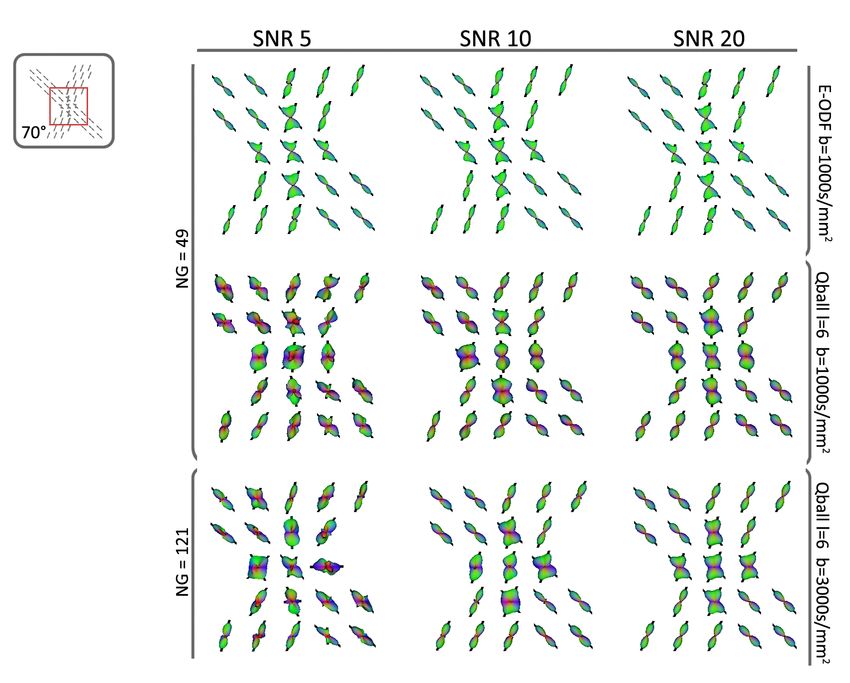
Fig. 2. E-ODFs and Qballs for different angles of crossing at fixed SN R = 20
for b = 1000s/mm2 , and SNR=10 for b = 3000s/mm2 . The Qballs at b =
3000s/mm2 are regularized with LB smoothing with λ = 0.006.
table 1. In the following paragraphs we relate them to some figures of interesting
parameter configurations and discuss the results. In figure 2, we present the
results of the performance of the proposed E-ODFs compared to the Qballs [15]
for different angles of crossings, and different simulation parameters: 49 gradient
directions, b-value 1000 s/mm2 and SNR 20, (figure 2 middle row) ; 121 gradient
directions, b-value 3000 s/mm2 , LB smoothing with λ = 0.006 [15] and SNR 10
(figure 2 third row).
We observe that for the angle of 50◦ , E-ODFs and not regularized Qballs
fail to find multiple maxima in the crossing areas. Only regularized Qball at
high b = 3000s/mm2 and high order l = 8, detects multiple maxima. For the(a) (b)
Fig. 3. Angular error and standard deviation for (a) E-ODFs at b = 1000s/mm2
and 49 gradient directions (b) Regularized Qball with λ = 0.006, b = 3000s/mm2
and 121 gradient directions.
angle of 60◦ the performance of E-ODFs is similar to the un-regularized Qball at
b = 1000s/mm2 and truncated at order of spherical harmonics l = 6. Regularized
Qballs at b = 3000s/mm2 outperform in this scenario. At an angle of 70◦ , the E-
ODFs outperform the best (un-regularized ) Qball scenario at order l = 8. Only
regularized Qball at l = 6 outperforms in this scenario (see table of figure 1).
The plots of figure 3.1 report the relation between the angular error and
change in SNR. We observe that the E-ODFs are more stable, regardless the
noise level, whereas the regularized Qballs improve significantly at higher SNRs.
However, it is important to note that in real data at high b-value ≈ 3000s/mm2
the SNR drops off to 5 (however, this might change depending on the type of
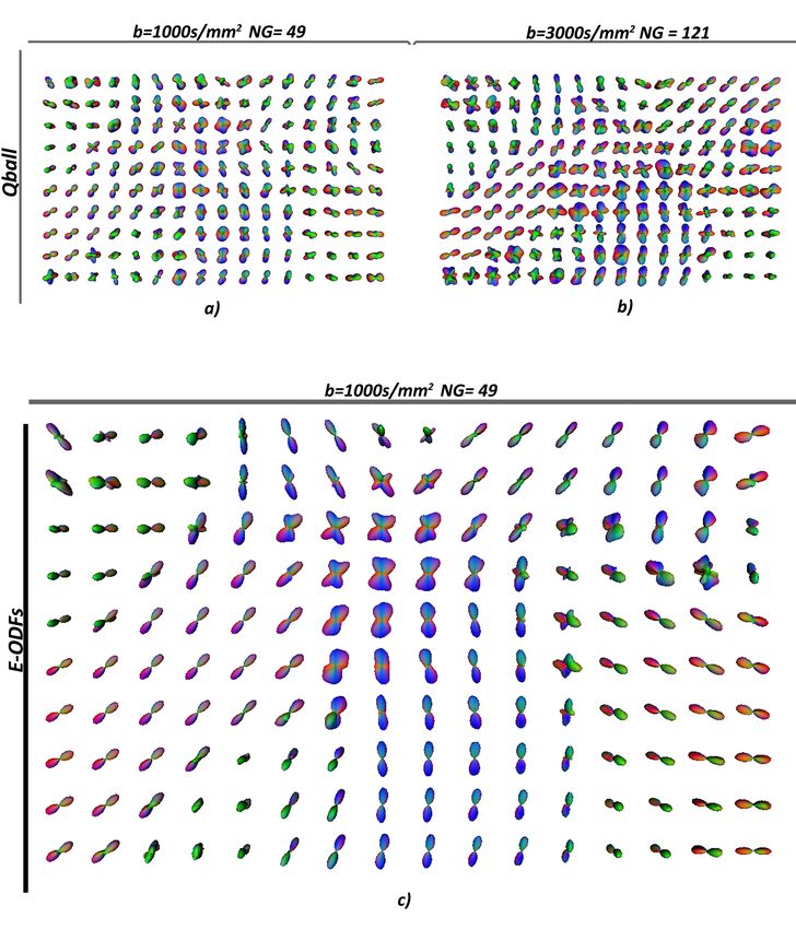
scanner and imaging parameters). Figure 4 illustrates the previous conclusions.
At higher order of truncation un-regularized Qball performs much worse, giving
many false positives in the linear areas where the SNR is low.
We observe that regardless the SNR, the E-ODFs preserve the coherence of
the linear and crossing regions, and preserve the angular error, to almost constant
(see figure 3(a)). We also compared the E-ODFs, to Qball’s best case scenario
with LB regularization [15]. Here, for SNR 5, Qball performs worse (angular
error of 14.9◦ and standard deviation 8.4◦ ) than the E-ODFs. As noise decreases,
E-ODFs’ performance is similar to the regularized Qballs at b = 3000s/mm2 (an-
gular error 9.8◦ and standard deviation 9.15◦ ). Regularized Qball outperforms
E-ODFs, for SNR 20, with an angular error of 5.15◦ and standard deviation of
3.2◦ . However, this SNR is not realistic given nowadays acquisition protocols
and machinery at b-values as high as 3000s/mm2 .Fig. 4. E-ODFs and Qballs for different SNRs, and different b-value, at fixed
angle of 70◦ .
3.2 Real data results
Even though crossing information is missing in the original DTI data, as well as
in the created ODFs (as can be seen in figure 5(a) and figure 5(b)), we observe
that after processing, crossing information is extrapolated (see figure 6(c)). The
obtained crossings are very much comparable to the Qball reconstructions of
l = 6, at b = 3000s/mm2 and 121 gradient directions and regularized with
LB smoothing of λ = 0.006 (figure 6(b)). The un-regularized Qballs at low b-
value of 1000s/mm2 and low gradient sampling of 49 gradient directions, present
less obvious structures of the CC and CR, and have more chaotically oriented
crossings, figure 6(a).
All computations were conducted in an AMD Athlon X2 Dual 2.41GHz,
with 3GB of RAM, taking 0.5 minutes per artificial tube dataset, and about 13
minutes for the real human brain dataset for estimating the E-ODFs.
4 Conclusions and Future Work
In this work we presented a method for extrapolating crossing information using
image processing of the coupled space of positions and orientations in DTI data.Fig. 5. The centrum semiovale. Left: the original DTI data, color coded by F A.
Right: the ODFs from the DTI data, RGB color coded by orientation and min-
max normalized.
We show that with typical acquisition schemes for DTI, the inferred fiber cross-
ings are similar to the crossings from 6th order un-regularized Qball estimated
from the same data. Furthermore we compare the E-ODFs to the best scenario
of Qball at typical HARDI acquisition schemes, and we conclude that the infor-
mation gain from the regularized Qball is similar at low SNR, but the Qballs
improve when increasing the SNR. However, in practice HARDI acquisitions at
high b-values result in very noisy datasets, and Qball reconstructions of poor
quality including LB regularization. The robustness to noise of the presented
method is significantly better than from the un-regularized Qballs reconstructed
from the same data, and comparable to the Qball’s best scenario. The main
contribution from this work lies on demonstrating similar quality of detected
crossings with modest acquisitions modeled by DTI, and with the use of con-
textual information as in the popular HARDI reconstruction techniques that
require more expensive acquisitions such as Qball. Future work addresses sim-
ilar comparison to spherical deconvolution [8] as well as tensor decomposition
techniques [21] which has proven to more reliably infer number and directions of
fibers. The chosen kernel sets an overall reasonable probabilistic model that gov-
erns how the context of a fiber fragment is taken into account. Consequently, our
framework lacks adaptivity. Future work will address more adaptive fiber con-
text models to the data, such that context is only included where it is required
by the data.
The method proposed has its limitations, it assumes that enough context is
available for a correct extrapolation. The possible implications of this limitations
for concrete brain structures should be studied. Future work should additionally
bear more extensive validation to assess the exact differences between HARDIFig. 6. Different profiles in the centrum semiovale a) un-regularized Qball of order 4 b) Regularized Qball with λ = 0.006 of order 6 from similar region as (a) c) E-ODFs of the same region as (a). models and E-ODFs concerning acquisition parameters and anatomical areas of the brain. This includes synthetic data experiments with fibers of different configurations (e.g. curved bundles) and multiple crossings. As a conclusion, contextual processing of DTI data allows overcoming one of the main drawbacks of the DT model. The crossing information can be recovered with an acquisition that typically takes 3-6 minutes and modest post-processing (13 minutes for 10
slices of a human brain on a standard PC). This gives future work potential for
applying more accurate stream-based tractography for DTI data.
References
 1. Basser, P.J., Mattiello, J., Lebihan, D.: MR diffusion tensor spectroscopy and
    imaging. Biophys. J. 66(1) (January 1994) 259–267
 2. Jones, D.K.: The effect of gradient sampling schemes on measures derived from
    diffusion tensor mri: a monte carlo study. MRM 51(4) (2004) 807–15
 3. Tuch, D.S.: Diffusion MRI of complex tissue structure. PhD thesis, Harvard (2002)
 4. Frank, L.R.: Characterization of anisotropy in high angular resolution diffusion-
    weighted MRI. MRM 47(6) (2002) 1083–99
 5. Alexander, D.C., Barker, G.J., Arridge, S.R.: Detection and modeling of non-
    gaussian apparent diffusion coefficient profiles in human brain data. MRM 48(2)
    (2002) 331–40
 6. Tuch, D.: Q-ball imaging. MRM 52 (2004) 1358–1372
 7. Özarslan, E., Shepherd, T.M., Vemuri, B.C., Blackband, S.J., Mareci, T.H.: Reso-
    lution of complex tissue microarchitecture using the diffusion orientation transform
    (DOT). NeuroImage 36(3) (July 2006) 1086–1103
 8. Tournier, J.D., Calamante, F., Connelly, A.: Robust determination of the fibre ori-
    entation distribution in diffusion MRI: non-negativity constrained super-resolved
    spherical deconvolution. NeuroImage 35(4) (2007) 1459–72
 9. Jian, B., Vemuri, B.C.: A unified computational framework for deconvolution to
    reconstruct multiple fibers from Diffusion Weighted MRI. IEEE Transactions on
    Medical Imaging 26(11) (2007) 1464–1471
10. Descoteaux, M.: High Angular Resolution Diffusion MRI: From Local Estima-
    tion to Segmentation and Tractography. PhD thesis, Universite de Nice - Sophia
    Antipolis (February 2008)
11. Liu, C., Bammer, R., Acar, B., Moseley, M.E.: Characterizing non-gaussian diffu-
    sion by using generalized diffusion tensors. MRM 51(5) (2004) 924–37
12. A. Barmpoutis, B. C. Vemuri, D.H., Forder, J.R.: Extracting tractosemas from
    a displacement probability field for tractography in DW-MRI. In LNCS 5241,
    MICCAI (6-10 September 2008) 9–16
13. Duits, R., Franken, E.: Left-invariant diffusions on R3 o S 2 and their application
    to crossing-preserving smoothing on HARDI-images. CASA report, TU/e, nr.18
14. Rodrigues, P.R., Duits, R., ter Haar Romeny, B., Vilanova, A.: Accelerated diffu-
    sion operators for enhancing DW-MRI. In: VCBM, Leipzig, Germany (2010)
15. Descoteaux, M., Angelino, E., Fitzgibbons, S., Deriche, R.: Regularized, fast and
    robust analytical Q-Ball imaging. MRM 58 (2007) 497–510
16. Basser, P.J., Mattiello, J., Lebihan, D.: Estimation of the effective self-diffusion
    tensor from the NMR spin echo. J. of Magn. Res. Series B 103 (1994) 247–254
17. Duits, R., Franken, E.: Left-invariant diffusions on the space of positions and orien-
    tations and their application to crossing-preserving smoothing of HARDI images.
    International Journal of Computer Vision 2010
18. Prčkovska, V., Roebroeck, A.F., Pullens, W., Vilanova, A., ter Haar Romeny, B.M.:
    Optimal acquisition schemes in high angular resolution diffusion weighted imaging.
    In: MICCAI. Volume 5242 of LNCS., Springer (2008) 9–17
19. Lagana, M., Rovaris, M., Ceccarelli, A., Venturelli, C., Marini, S., Baselli, G.:
    DTI parameter optimisation for acquisition at 1.5T: SNR analysis and clinical
    application. Comput Intell Neurosci NIL(NIL) (2010) 254032
20. Jones, D., Horsfield, M., Simmons, A.: Optimal strategies for measuring diffusion
    in anisotropic systems by magnetic resonance imaging. MRM 42 (1999) 515–525
21. Schultz, T., Seidel, H.P.: Estimating crossing fibers: A tensor decomposition ap-
    proach. IEEE Transactions on Visualization and Computer Graphics 14 (2008)
    1635–1642
You can also read