How to evaluate synthetic radar data? Lessons learned from finding driveable space in virtual environments - Uni-DAS
←
→
Page content transcription
If your browser does not render page correctly, please read the page content below
How to evaluate synthetic radar data? Lessons learned
 from finding driveable space in virtual environments
        Martin F. Holder∗ , Jan R. Thielmann† , Philipp Rosenberger∗ ,
                  Clemens Linnhoff∗ , and Hermann Winner‡

Abstract: Generating synthetic sensor readings at scale by means of virtual sensors is expected
to facilitate safety validation of autonomous driving functions. An absolute equality of real and
synthetic data is not to be expected. Instead, it has to be proven that synthetic sensor data
exhibits a comparable level of uncertainties as data from the real sensor, so that subsequent
algorithms draw the same conclusions from the respective input data. This paper addresses
this problem by comparing free space information inferred from real and synthetic radar data.
It is shown that comparable free space can be calculated from the sensor simulation, although
deviations between synthetic and real sensor data exist. The presented method to compare the
calculated free space from synthetic and real data serves as evaluation of the simulation model.
Keywords: Automotive Radar, Sensor Modeling, Environment Perception, Virtual Validation

1       Introduction
During development of sensor simulation models for virtual validation of autonomous
driving, it is of interest to identify the current performance level of the model. When
generating synthetic sensor data as available from an implementation of a sensor model
from a simulation environment such as IPG Carmaker, Vires Virtual Test Drive, CARLA
etc., differences to measured data are naturally expected as models are always only an
approximation to reality. Especially for the simulation of environmental sensors, the
achievable accuracy of the virtual representation is limited: Detailed modeling of reflection
properties of materials is an open research topic and modeling radar sensors is known to
be particular challenging [1]. Besides, once a sensor simulation model is implemented,
uncertainties in its parameterization remain. For example, uncertainty regarding main
radar performance parameters, such as measurement ranges, window functions, antenna
gains but also mounting position etc. is present and this uncertainty in the model is part
of the overall epistemic uncertainty. Next, the parameter space of the virtual environment,
in which the sensor model is executed, revolves around reflection properties of materials,
    ∗
     Martin Holder M. Sc., Philipp Rosenberger M. Sc., and Clemens Linnhoff M. Sc.              are
Research Associates at Institute of Automotive Engineering (FZD) at TU Darmstadt, E-Mail
(holder,rosenberger,linnhoff@fzd.tu-darmstadt.de).
   †
     Jan Thielmann M. Sc. conducted his Master’s Thesis at the Institute of Automotive Engineering
(FZD) at TU Darmstadt, E-Mail (janthielmann@gmx.de).
   ‡
     Prof. Dr. rer. nat. Hermann Winner is Head of Institute of Automotive Engineering (FZD) at TU
Darmstadt, E-Mail (winner@fzd.tu-darmstadt.de).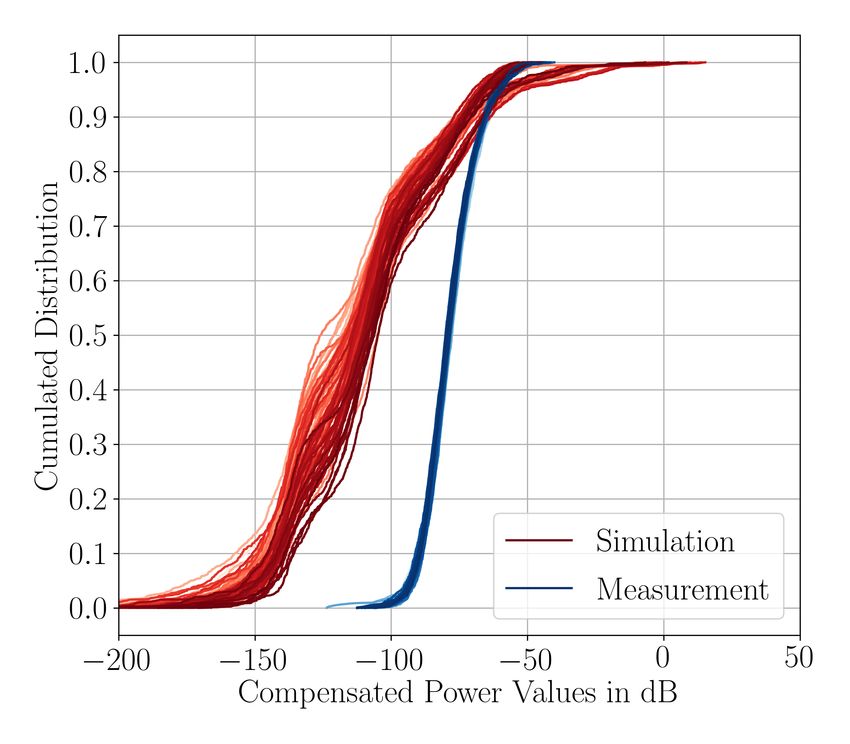
such as objects, vegetation, pavement, etc., but also includes the virtual scenery itself
with arbitrary level of complexity of the 3D models with respect to resolution and details.
Since absolute equality of simulated and real values is never to be expected, methods are
researched to evaluate a simulation model. An ad-hoc solution for model validation is to
stimulate subsequent algorithms in the sensor data processing pipeline with both real and
synthetic data and observe the amount of consensus, similar to the concept of runtime
verification [2], which is subject of this work.

2     Comparing Synthetic and Real Radar Sensor Data
Already during model development, tools are needed to check the correct implementation
(verification) and to make a statement about the degree of functional fulfillment of the
requirements of the model (validation). On the one hand, it has to be proven that
basic radar sensor parameters such as the measuring ranges in distance, azimuth and
relative speed are correctly modeled. On the other hand, a model is considered falsified
if the conclusions drawn by data processing algorithm from synthetic and real data are
contradictory. For example, synthetic radar data could be fed into an object tracking
algorithm and the results evaluated using specific metrics. In the sense of validating
a simulation model, it would be considered (sample-)valid if the score achieved for a
metric was within predefined limits [3]. However, this is difficult for many reasons: The
data processing algorithms usually comprise a large number of parameters whose optimal
choice must first be found. Second, it must be proven that these parameters can be
transferred into the simulation to guarantee the equivalence of the algorithm. Ultimately,
the comparison by means of (validated) metrics assumes that their calibration has already
been performed. To the best of the authors’ knowledge, no validity criteria are available
for radar sensor models using metric-based key figures. This makes an objective evaluation
of the quality of a sensor simulation more complicated and demands for new methods.

2.1    Grid Maps as Tool for Sensor Model Evaluation
The idea laid out in this paper is to initially allow for derivations between synthetic
and measured radar sensor readings and shift the task of judging about the validity and
meaningfulness of the synthetic data to subsequent data processing algorithms. The
methodological approach is to recreate a test drive that was conducted in real world,
in a virtual environment and then calculating the free space that is computed from the
occupancy grid map and is available for planning in the scenery. Free space determination
with Occupancy Grid Maps (OGM) based on Radar sensors has been extensively studied [4–
7] and promises to avoid the challenges mentioned above: In OGM the Inverse Sensor
Model (ISM) translates sensor readings into probabilities for occupancy of a specific grid
cell. By evaluating the cumulative distribution of the sensor readings, the ISM adjusts its
parameters accordingly. This facilitates comparison of synthetic to real data for evaluating
environment occupancy. Comparison of OGM can be done either with heuristics [8], but
this would again require calibrated metrics. In addition, a baseline offset is expected,
since a real scene can only be reproduced in a simulation environment with finite and
difficult to quantify accuracy. Instead, it should be checked whether essential information
about free space is also contained in the synthetic data and whether a comparable path
for a self-driving vehicle is available in the free space. In order to compare synthetic
and real data, this paper’s working hypothesis is stated as: Despite inaccuracies in the
modeling, the free space that can be detected by a radar sensor is similarly reproduced in
simulation. It can be falsified if no similar path through free space could be derived from
the OGM calculated from real or synthetic data. The hypothesis can also be understood
as a qualitative requirement for a sensor simulation that a model must meet in order to
be considered acceptable for simulation-based testing. Since the focus of this work is on
the comparison of real and synthetic radar data, the pipeline for calculating free space is
designed with fairly simple algorithmic components, see Figure 1.

  Conducted in real world                         From measurement
  experiment or simulation                           or simulation
                                                                                              OGM Algorithm
                              Apperance                                     Antenna gain
      Scenery and              to sensor            Sensor                  compensation      Inverse Sensor
        Scenario                                   Readings                                       Model
                                                                                Discretization to grid and
 Meaningful driveable path?
                                                                              cell occupancy probabilities
                         A∗ path finding in interval based representation

                                                  Free Space                                 Dempster-Shafer
       Planning
                               Driveable region   Estimation                Occupied cells     Grid Map

Figure 1: Road map for evaluation of synthetic sensor data: In both measurement and
simulation, a scenery is observed by a radar sensor and its measurements are fed into
an OGM algorithm. Free space and a driveable path are searched and their feasibility is
evaluated.

2.2     Radar Measurements and Simulation
Automotive radar often uses chirp sequence waveforms with a patch antenna array. Subse-
quent Fourier transformations over each chirp, the sequence of chirps, and the antennas
deliver a three dimensional spectrum, where each bin contains the spectral power for a
certain range, range-rate, and azimuth bin. This data type is also called radar cube and
can be seen as raw radar data where no thresholding has been applied. Basically, it is
available for all chirp sequence radars with digital beamforming and a modeling approach
that renders synthetic data on this interface has been proposed in earlier work by the
authors [9], which motivates its usage in this work.

2.3     From Occupancy Grid Mapping to Driveable Path from a
        Free Space Estimate
The ISM represents grid-based environment occupancy in the posterior probability for
occupancy of a grid cell Oj for a given power reading at cell j from the sensor PTx,j
and vehicle pose zj . Raw radar data is notoriously difficult to interpret because of
several pertinent artifacts, such as noise, ambiguities, and limited resolution. Aleatoric
uncertainties are inherently present in this kind of data, simply due to the physical
measurement principle of the radar: Due to multipath propagation and noise artifacts in
the radar, the area between the sensor and the obstacle cannot necessarily be considered
free based on the sensor readings, although there is no real obstacle. In the sensor
measurement, this is initially only reflected in areas with increased received power, for
which the occupancy is justified via the ISM. Although the radar shows a better penetration
of optical occlusions, it can be argued that a radar measurement can be better used to
determine the occupied areas than to infer free space. The ISM proposed by [10] is used in
this paper: It is parameterized from the empirical distribution of received power values. For
capturing pure measurement noise, the lower threshold, PTx,0.1 , is found as the upper limit
of the 10 % of the lowest observed values in the cumulative distribution power readings.
Actual obstacles like cars are expected to show high power readings and therefore the
upper threshold, while PTx,0.9 is the lower limit of 90 % of the largest observed values in
the current measurement frame. The intermediate region is assumed to consist of large
clutter targets as well as weak reflections from the terrain. In order to compensate for
the directional dependence of the received power, it is equalized with the antenna gain
characteristics. Consequently, the ISM requires a certain dynamic range between minimum
and maximum power values in order to determine occupancy probabilities. The ISM and
the cumulative distribution of the received power is illustrated in Figure 2.
1
0.9 1
0.7 0.8
0.6
0.5
0.4
0.3 0.2
0.1 0
0
-200 -150 -100 PTx, 0.1 PTx, 0.9 100 150
Figure 2: Schematic illustration of the proposed ISM based on the distribution of PTx .
The Dempster-Shafer Theory (DST) is a decision-making strategy that differentiates
lack of information from conflicting or uncertain information, which makes it attractive
for map building [11, 12]. In the OGM that is calculated from DST, the interval-based
method [13] is used for obtaining free space from an occupancy grid map. This method is
characterized by being computationally inexpensive and non-parametric: While it does not
guarantee an optimal solution for obtaining free space it is easier to implement compared
to parametric methods like B-splines [14]. The A∗ path-finding algorithm is used to search
a (driveable) path within the estimated free space that would be available for trajectory
planning. For a passable path a minimum width of 2 cells and a minimum clearance of
one cell from an obstacle is required.2.4 Evaluation Aspects of OGM for Sensor Modeling
Two aspects of sensor modeling are evaluated via the OGM and the calculation of the
free space: On the one hand, the dynamic range of the simulated sensor can be compared
to the measurement results in order to evaluate whether the ISM is able to correctly
calculate gradations in the probability of occupancy. On the other hand, the detailing of
the environment is evaluated: In the proposed scenarios the modeling of the road edge
is of interest, since the irregularity of the vegetation, as it exists in reality, can only be
represented with an unreasonable effort in the virtual image of the environment. For this
reason, a simple substitute modeling is used in the simulation model, which consists of a
homogeneous vegetation strip along the line. Due to this (intentional) modeling inaccuracy,
deviations in the free space are to be expected. An examination of the required faithfulness
of the vegetation rendering would be possible in order to make a statement about the
required degree of detailing.
3 Experiments
A far range radar with a measurement range of 200 m and approx. 25◦ in azimuth is used
in real-world experiments. The first 15 m in front of the radar are excluded since they are
assumed to contain only clutter reflections from the road. A respective simulation model
has been parametrized according to this sensor. The size of a grid cell balances between
the measurement accuracy of the sensor and the resulting total size of the grid. In order to
take into account the range of the long-range radar with the limited lateral measurement
range, a grid cell of 1 m was selected. Grid sizes of approx. 10 cm are common in lidar
applications [15] and a similar grid size could be achieved with higher resolution radar
sensors. With respect to the planning algorithm, it is expected to find a feasible trajectory
for a regular passenger car within the required width of two cells.
Ego Target
Ego
(a) Free runway (b) Occupied ego-lane
Figure 3: Illustration of the evaluation scenarios
Two experiments have been performed at the August Euler airfield in Griesheim, with
its runway having a width of approx. 20 m, which corresponds to a width of 20 grid cells,
see Figure 3. The first scenario involves a free runway and is used for evaluating the
general capability of the pipeline to infer free space and learn about the accuracy of the
environment simulation. Here, the ego vehicle drives straight ahead on the runway and
the free space is therefore only limited by the vegetation at the roadside. In the second
scenario, a target vehicle is located on the same lane as the ego vehicle. The target vehicle
moves (slowly) away from the ego vehicle but overtaking through the left lane would bepossible at any time. The purpose of the experiment is to determine at which point both
the simulation and the measurement, based on the free space recorded, would consider an
overtaking attempt as possible.
4 Results
4.1 Sensitivity of PTx
The core element of free space estimation is the inverse sensor model. As mentioned at
the beginning, this requires a certain dynamic range between minimum and maximum
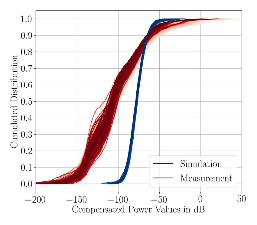
power which is examined for both scenarios. Figure 4 shows the cumulative distribution
of all received power values,PTx , during both scenarios.
(a) Free Runway (b) Occupied ego-lane
Figure 4: Cumulative Distribution of received power values for both scenarios. Individual
time-steps are marked by darker color. The temporal process is coded in the color intensity.
The darker, the more advanced the time.
As expected, the dynamic range in the measurement is increased due to the presence
of the target vehicle in the second scenario. Basically, the measurement shows a similar
course for both scenarios. Like the measurement, higher received power is sensed in the
second scenario due to the presence of the target vehicle. With the empirical distribution
the following aspects of the simulation can be falsified: The spread shows that the noise
behavior is much more significant in the simulation than in the measurement. A higher
dynamic range in the simulation shows that the simulated received power covers a higher
bandwidth. The deviation of the median value indicates that the received power of
weak targets such as vegetation is incorrectly simulated. Despite the differences, the
synthetic data shows sufficient dynamics so that the ISM can parameterize itself and assign
occupancy probabilities to the received power readings.4.2 Free Runway Scenario
Figure 5 shows a qualitative comparison of the received power PTx , the probability of
cell occupancy P (Oj ) and the free space derived from it along with the proposed path.
Simulated quantities are denoted with [ ˜ ].
Obviously, deviations between simulation and measurement can already be detected
in the comparison of the received power. Particularly noticeable in the synthetic data
is the increased visibility of the edge of the road even at larger distances. A narrower
width of the roadway is visible in the free space map because the lateral expansion of the
reflections from the edge of the roadway is more significant in the synthetic data. Despite
the deviations, in both cases it is possible to plan the (trivial) path, the straight route.
PTx P(Oj )
Azimuth 1
min max 200
200 max
0.8
175
150
150
0.6
125
Oy
100
100
0.4
75
50
50 0.2
25
0 0
0 min
−40 −20 0 20 40
Range in m Ox
(a) Received power from (b) Occupancy grid with (c) Freespace (green) and path
measurement measured data (blue) for measured data
P̃Tx
P̃(Oj )
min
Azimuth
max 200 1
200 max
175 0.8
150
150
0.6
125
Õ y
100
100
0.4
75
50
50 0.2
25
0 0
−40 −20 0 20 40
0 min
Range in m Õ x
(d) Received power from (e) Occupancy grid with (f) Freespace (green) and path
simulation synthetic data (blue) for synthetic data
Figure 5: Qualitative comparison of measurement (top) and simulation (bottom) results
for the free runway scenario.4.3 Occupied Ego-lane Scenario
The task in this scenario is to find a path around the vehicle in front, which can be done by
switching to the free left lane on the left. Through spectral windowing the vehicle smears
in azimuthal direction, so that some azimuth cells are marked as occupied. Therefore, the
sensor will only be able to capture the free space and plan a path around the vehicle after
a certain distance. By comparing the required minimum distance from simulation and
measurement, it is possible to evaluate the extent to which the window effects mentioned
are correctly implemented in the simulation model. The definition of passability is shown
in Figure 6. It should be noted that only the passability of the free space estimated by
the sensor is considered and the target’s backscattering is sufficiently high, see Figure 6c,
where overtaking is possible, but is intentionally prevented for illustrative purposes.
(a) No path for overtaking (b) Reasonable path for over- (c) Visibility of the target at
found taking found distance
Figure 6: Illustrative definition of a passable path
Figure 7 illustrates the distances at which sufficient space for overtaking is estimated
on the left lane. Both measurement and simulation show sporadic time steps up to a
distance of about 130 m, at which an overtaking path can be planned. At very close range,
overtaking is not considered possible due to the limited visibility of the radar. Although
the measurement still shows a few isolated time steps from 130 m upwards to which no
path can be found, these can be traced back to noise effects. Deviating from the simulation,
the measurement in the intermediate area shows a clearly more unsteady pattern with
regard to the overtaking possibility. Because of the slow speed of the target vehicle, this is
caused by interference patterns that cannot be found in the simulation in this form.
Yes
Passable Path?
No
Yes
Measurement
Simulation
No
0 25 50 75 100 125 150 175 200
Distance to Ego in m
Figure 7: Comparison of the distance of the target to the ego vehicle at which a path for
overtaking exists according to radar measurements.5 Implications for Radar Sensor Modeling Based on the results obtained, there are a number of implications for sensor modeling: First, the sensitivity analysis of the received power shows differences in dynamic range for synthetic data and reveals differences in noise behavior. The dynamics of real radar data is limited at the lower end by the noise level and at the upper end by the maximum level at the AD converter. The simulation model used in this paper shows no such dynamics limitation. In fact, this does not exist naturally for virtual sensors, since for example in raytracing based approaches, the signal strength of a ray can initially become arbitrarily small during propagation and reflection. For this application, this is of secondary importance due to the self-parameterization of the ISM to the cumulative power distribution. However, other applications, such as CFAR algorithms, make more restrictive assumptions about the signal-to-noise ratio, so that this must be taken into account in a simulation model. With regard to model parameters, the investigation shows the importance of correct modeling of azimuthal blurring as a consequence of spectral window effects in the azimuth direction. As the first experiment has shown, the free space in lateral direction at larger distances is incorrectly reproduced with the sensor model used in this work. Free space that can be detected by a sensor simulation model is closely linked to the accuracy of the environmental simulation. The results show that the design of the boundary area, i.e. the transition between the passable area and the vegetation, is of great importance. The simple vegetation model in the simulation already exhibits a well comparable shape of the OGM at the boundary area. This may serve as a first evidence for required detailing of such areas for radar sensor modeling. 6 Conclusion This paper presents a method for evaluating a radar sensor simulation model by comparing the driveable space: By feeding synthetic data into an algorithm developed for real data, the strengths and weaknesses of a sensor simulation model can be investigated. The initial situation was that deviations between measurement and simulation were initially allowed, but the consequences related to the planning of a passable path were examined in two scenarios. Despite differences in the absolute value of simulated data, it is possible to evaluate a sensor model using the method presented: The advantage of the presented method is that initially deviations between synthetic and real data are allowed, because only the dynamic range is relevant for the parameterization of the ISM which results in a robustness against statistical deviations in the input data. By comparing the cumulative distributions of received power, model assumptions can also be falsified. The developed method is an extension to the research for the validation of sensor models and serves as a tool for testing the sensor model and its implementation in virtual environments. 7 Acknowledgement This research is funded by the SET Level 4to5 research initiative, promoted by the Federal Ministry for Economic Affairs and Energy (BMWi). The authors would like to thank Albert Schotschneider for his support in the development and implementation of the algorithms.
References
 [1] M. Holder, P. Rosenberger, H. Winner, T. Dhondt, V. P. Makkapati, M. Maier, H.
     Schreiber, Z. Magosi, Z. Slavik, O. Bringmann, and W. Rosenstiel, “Measurements
     revealing Challenges in Radar Sensor Modeling for Virtual Validation of Autonomous
     Driving”, in 2018 21st International Conference on Intelligent Transportation Systems
     (ITSC), Nov. 2018.
 [2] E. Bartocci and Y. Falcone, Eds., Lectures on Runtime Verification. Springer Inter-
     national Publishing, 2018.
 [3] P. Rosenberger, J. T. Wendler, M. F. Holder, C. Linnhoff, M. Berghöfer, H. Winner,
     and M. Maurer, “Towards a Generally Accepted Validation Methodology for Sensor
     Models - Challenges, Metrics, and First Results”, in Grazer Symposium Virtuelles
     Fahrzeug, May 2019.
 [4] K. Werber, M. Rapp, J. Klappstein, M. Hahn, J. Dickmann, K. Dietmayer, and C.
     Waldschmidt, “Automotive radar gridmap representations”, in 2015 IEEE MTT-S
     International Conference on Microwaves for Intelligent Mobility (ICMIM), Apr.
     2015.
 [5] J. Lombacher, K. Laudt, M. Hahn, J. Dickmann, and C. Wohler, “Semantic radar
     grids”, in 2017 IEEE Intelligent Vehicles Symposium (IV), Jun. 2017.
 [6] R. Weston, S. Cen, P. Newman, and I. Posner, “Probably Unknown: Deep Inverse Sen-
     sor Modelling Radar”, in 2019 International Conference on Robotics and Automation
     (ICRA), May 2019.
 [7] M. Holder, S. Hellwig, and H. Winner, “Real-Time Pose Graph SLAM based on
     Radar”, in 2019 IEEE Intelligent Vehicles Symposium (IV), Jun. 2019.
 [8] T. Colleens, J. Colleens, and D. Ryan, “Occupancy grid mapping: An empirical
     evaluation”, in 2007 Mediterranean Conference on Control & Automation, Jun. 2007.
 [9] M. Holder, C. Linnhoff, P. Rosenberger, and H. Winner, “The Fourier Tracing
     Approach for Modeling Automotive Radar Sensors”, in 2019 20th International
     Radar Symposium (IRS), Jun. 2019.
[10] M. Li, Z. Feng, M. Stolz, M. Kunert, R. Henze, and F. Küçükay, “High Resolution
     Radar-based Occupancy Grid Mapping and Free Space Detection”, in VEHITS,
     2018.
[11] D. Pagac, E. Nebot, and H. Durrant-Whyte, “An evidential approach to map-building
     for autonomous vehicles”, IEEE Transactions on Robotics and Automation, vol. 14,
     no. 4, pp. 623–629, 1998.
[12] R. Murphy, “Dempster-Shafer theory for sensor fusion in autonomous mobile robots”,
     IEEE Transactions on Robotics and Automation, vol. 14, no. 2, pp. 197–206, Apr.
     1998.
[13] T. Weiherer, S. Bouzouraa, and U. Hofmann, “An interval based representation of
     occupancy information for driver assistance systems”, in 16th International IEEE
     Conference on Intelligent Transportation Systems (ITSC 2013), Oct. 2013.
[14] M. Schreier, V. Willert, and J. Adamy, “Compact Representation of Dynamic Driving
Environments for ADAS by Parametric Free Space and Dynamic Object Maps”,
IEEE Transactions on Intelligent Transportation Systems, vol. 17, no. 2, pp. 367–384,
Feb. 2016.
[15] J. Porebski, K. Kogut, P. Markiewicz, and P. Skruch, “Occupancy grid for static
environment perception in series automotive applications”, IFAC-PapersOnLine,
vol. 52, no. 8, pp. 148–153, 2019.You can also read