Finite element simulations of hybrid nano Carreau Yasuda fluid with hall and ion slip forces over rotating heated porous cone
←
→
Page content transcription
If your browser does not render page correctly, please read the page content below
www.nature.com/scientificreports
OPEN Finite element simulations
of hybrid nano‑Carreau Yasuda
fluid with hall and ion slip forces
over rotating heated porous cone
Umar Nazir1, Muhammad Sohail1*, Mahmoud M. Selim2,3, Hussam Alrabaiah4,5 &
Poom Kumam6,7*
Involvement of hybrid nanoparticles a vital role to improve the efficiency of thermal systems. This
report covers the utilization of different nanoparticles mixed in Carreau Yasuda material for the
improvement of thermal performance. The configuration of flow situation is considered over a rotating
porous cone by considering the Hall and Ion slip forces. Transport of momentum is considered to
be in a rotating cone under generalized ohm’s law and heat transfer is presented by considering
viscous dissipation, Joule heating and heat generation. Rheology of considered model is derived
by engaging the theory proposed by Prandtl. Modeled complex PDEs are reduced into ODEs under
similarity transformation. To study the physics behind this phenomenon, solution is essential. Here,
FEM (Finite Element Method) is adopted to compute the solution. Furthermore, the grid independent
study is reported with several graphs and tables which are prepared to note the influence of involved
parameters on thermal and velocity fields. It is worth mentioning that heat transport is controlled via
higher radiation parameter and it upsurges for Eckert number. Moreover, Hall and ion slip parameters
are considered significant parameters to produce the enhancement in motion of fluid particles but
speed of nano and hybrid nanoparticles becomes slow down versus large values of Forchheimer and
Weissenberg numbers. Additionally, an enhancement in production of heat energy is addressed via
large values of heat generation number and Eckert number while reduction in heat energy is occurred
due to positive values of thermal radiation and Hall and ion slip parameters.
Flow over a rotating geometries got considerable attention by the researchers due to their wider applications in
numerous technological developments instruments and appliances. Inclusion/mixing of hybrid nanoparticles
is highly recommended by the engineers to improve the thermal performance. Many rheological relations have
been proposed by the researchers to study transport phenomenon. An important relation of Carreau-Yasuda
model1–5 is
n−1
d
ηCY (γ̇ ) = µ∞ + (µ0 − µ∞ ) 1 + (ϒ γ̇ )d .
For ϒ = 0 or n = 1, Newtonian model is recovered. Due to diverse applications, this model got the remark-
able attention and attraction by different researchers. For instance, Mahmood et al.1 presented the finite element
based computational analysis on Carreau-Yasuda model in a cavity with obstacle. They plotted the behavior of
influential fluid parameters and analyzed the tabular results for comparison purpose. They noted the depreciation
1
Department of Applied Mathematics and Statistics, Institute of Space Technology, P.O. Box 2750,
Islamabad 44000, Pakistan. 2Department of Mathematics, Al‑Aflaj College of Science and Humanities Studies,
Prince Sattam Bin Abdulaziz University, Al‑Aflaj 710‑11912, Saudi Arabia. 3Department of Mathematics, Suez
Faculty of Science, Suez University, Suez 34891, Egypt. 4College of Engineering, Al Ain University, Al Ain,
UAE. 5Department of Mathematics, Tafila Technical University Tafila, At‑Tafilah, Jordan. 6Center of Excellence
in Theoretical and Computational Science (TaCS‑CoE) and KMUTT Fixed Point Research Laboratory, Room SCL
802 Fixed Point Laboratory, Science Laboratory Building, Departments of Mathematics, Faculty of Science,
King Mongkut’s University of Technology Thonburi (KMUTT), 126 Pracha‑Uthit Road, Bang Mod, Thung Khru,
Bangkok 10140, Thailand. 7Department of Medical Research, China Medical University Hospital, China Medical
University, Taichung 40402, Taiwan. *email: muhammad_sohail111@yahoo.com; poom.kum@kmutt.ac.th
Scientific Reports | (2021) 11:19604 | https://doi.org/10.1038/s41598-021-99116-z 1
Vol.:(0123456789)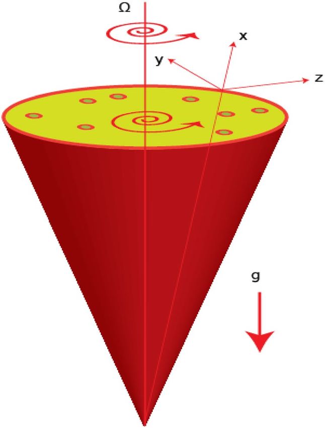
www.nature.com/scientificreports/
in viscosity of Carreau-Yasuda material by improving the relaxation time. Steady and oscillatory flow behavior
of Carreau-Yasuda material via Lattice Boltzmann procedure (LBP) was reported by Boyd and B uick2. They
discovered the different behavior in flow of Carreau-Yasuda material under different situations and assumptions.
Coclite et al.3 analyzed different impacts of Carreau-Yasuda material in a lid-driven cavity. Stability analysis
for Carreau-Yasuda material obeying poiseulle flow phenomenon via Chebyshev polynomial tool (CPT) was
explored by Pinarbasi and L iakopoulos4. Bio-convection phenomenon in radiated chemically reactive magnet-
ized slip of Carreau-Yasuda material was examined by Waqas et al.5. They engaged BVP4C package (MATLAB
COMPUTATIONAL PACKAGE) to compute solution of transformed modeled problem. Several important flow
features have been captured against numerous influential parameters. Results have been compared as a limiting
case current inspection with the published ones. They observed the decline in fluid velocity against Rayleigh
number and it escalates for Weissenberg parameter. Also, augmentation in thermal field is recorded against slip
parameter.
Thermal stability and mechanism of heat transportation is essential to study the thermal performance of
nanoparticles. Researchers have presented several models for the thermpophysical features of nanoparticles
and recorded their advantages and disadvantages. Inclusion of nanoparticles is a hot topic of research because
of their vast applications. One cannot avoid the use of nanoparticles. These coated particles are used in different
appliances and medical instruments for the treatment of patients suffering in different diseases. Several research-
ers paid attention on this direction. For instance, Darcy-Forchheimer flow of convective carbon water based
nanofluid immersed in a stretching cylinder with viscous dissipation, radiation, variable thermal conductivity
and obeying slip constraints was analyzed by Hayat et al.6 by engaging the model of thermophysical features
proposed by Xue. Solution to the governing modeled expressions has been approximated by shooting procedure.
They recorded the dual behavior of velocity and temperature fields against curvature parameter. Moreover, heat
transportation rate escalates against radiation parameter, whereas depreciation in skin friction is noted for grow-
ing Eckert number. Electrically conducting radiative stretched flow of convective incompressible nanofluid with
variable magnetic field was studied by Nayak et al.7 via shooting procedure. They presented the validation of
obtained solution by comparing the results. They recorded the diminution in thermal field for higher convection
parameter. Hady et al.8 presented the comparative analysis for convective nonlinear flow saturated in permeable
surface via numerically procedure. They displayed several results against numerous influential parameters. They
found the decrease in heat transportation rate for higher porosity parameter and an increase in skin friction.
Nonlinear chemically reactive flow of Maxwell nanofluid past over a rotating stretched surface with activation
energy was explored by Shafique et al.9. They used shooting method to obtain the solution of boundary layer
transformed ODEs. They observed the influence of several emerging parameters through graphs and tabular
data. They noted the enhancement in mass transfer rate for Schmidt number and depreciation in concentration
field. Utilization of SWCNTs and MWCNTs to improve the thermal performance of engine oil and water based
rotating viscous liquid with internal heating was examined by Rehman et al.10. They solved the resulting equa-
tions numerically and flow behavior is monitored through graphs and tabular data. They analyzed the higher
skin friction and heat transfer rate for engine oil based mixture as compared with water based mixture for both
MWCNTs and SWCNTs. Moreover, significant escalation in velocity field is recorded for higher volume fraction.
Seth et al.11 worked on nonlinear mixed convective flow of viscous liquid past over a nonlinear stretched surface
via FEM and OHAM. They considered velocity slip and performed regression analysis. They noticed the increase
in velocity for stagnation parameter and decrease in thermal profile. Kandasamy et al.12 developed alumunia
and copper based model to notice the thermal performance of mixed convective chemically reactive flow. They
used the thermophysical model proposed by Magyari and Mamut. They noticed the several important features
through plots. They monitored the rise in velocity for velocity slip parameter and opposite trend in concentra-
tion field. McCash et al.13 studied characteristics of viscous fluid inside two tubes using exact solution approach.
Zidan et al.14 discussed the thermal aspects of blood flow in multiple stenosis. They used exact approach to know
behavior of blood flow and entropy generation. Saleem et al.15 performed bio-mathematical scheme to know
behavior of blood flow in artery (non-symmetric and symmetric stenosed) including Joule heating. McCash
et al.16 modeled flow behavior of Peristaltic liquid inserting hybrid nanoparticles in an Elliptic Duct along with
advancing boundaries. Rehman et al.17 highlighted thermal aspects in pseudoplastic liquid inserting nanoparti-
cles over Riga heated surface considering thermophoresis diffusion and Brownian motion. They estimated surface
force, flow and heat energy using various physical parameters and numerically solved by numerical scheme.
Akhtar et al.18 discussed features of heat energy in non-Newtonian fluid including carbon nanotubes towards.
They used exact solution scheme to know aspects of pressure gradient, heat energy and flow phenomena inside
melting a vertical duct. Rizwana et al.19 scrutinized formulation of thermal aspects under the action of magnetic
field over oscillating melting plate inserting nanoparticles along with convective boundary conditions. Yasin
et al.20 discussed laminar flow in heated rods via finite element method approach. Ahmad et al.21 formulated
micropolar liquid suspending hybrid nanoparticles using non-Fourier’s theory considering triple stratification.
Yasin et al.22 used finite element approach to know aspects of Lorentz forces along with convective flow in adi-
abatic (enclosure). Hussain et al.23 formulated heat transfer in Carreau–yasuda liquid inserting nanoparticles
towards melting surface. Nazir et al.24 simulated comparative results of hybrid nanoparticles in Williamson
among nanoparticles and hybrid nanoparticles towards a meeting sheet using non-Fourier’s theory. In another
survey, Nazir et al.25 discussed comparison analysis in Carreau liquid among variable and constant viscosity via
non-Fourier’s theory numerically solved by FEA (finite element approach). Important studies contributing the
modeling of several phenomena under different flow conditions are reported i n26–31.
Available literature has no reported study by considering the inclusion of hybrid nanoparticles in Carreau-
Yasuda model with dissipation effect and engagement of Hall and ion slip forces in rotating porous cone. This
report will be used as a base for the researchers working further on Carreau-Yasuda model by engaging differ-
ent physical effects. This draft is organized as: comprehensive literature survey is included in Sect. 1, modeling
Scientific Reports | (2021) 11:19604 | https://doi.org/10.1038/s41598-021-99116-z 2
Vol:.(1234567890)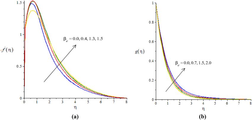
www.nature.com/scientificreports/
is mentioned in Sect. 2 along with important physical quantities, Sect. 3 contains the explanation of solution
scheme, graphical and tabular results are reported in Sect. 4 and important results have been listed in Sect. 5.
In future endeavors this work will be extended by considering following important effects.
• Slip effects, variable viscosity (space dependent/shear rate dependent/concentration dependent/temperature
dependent) and variable magnetic field;
• Mixed convection;
• Modified heat flux and radiation effect;
• Variable thermal conductivity;
• Space dependent heat source;
• Variable diffusion coefficient;
• Utilization of ternary hybrid nanoparticles mixture;
• Linear, nonlinear stretching sheets with and without porosity;
• CPU analysis of iteration of different schemes and comparative study.
Nomenclature
Symbols/units Used for Symbols/units Used for
z, x, y[m] Space coordinates Ec[no unit] Eckert number
u, v, w[ms−1] Velocity components Re[no unit] Reynolds number
G[Newton] Gravitational force nf Nano-fluid
Uw[ms−1] Wall velocity We[no unit] Weissenberg number
T [kelvin] Temperature field Hs Heat generation number
T∞ , Tw[kelvin] Ambient and wall temperatures Nu Nusselt number
B0[Oersted Ampere/meter] Magnetic field strength SiO2 Silicon dioxide
Cf , C g Skin friction coefficients T0[kelvin] Reference temperature
k[(W/(m⋅K))] Thermal conductivity Greek symbols
hnf , bf Hybrid nanofluid and base fluid α[radian] Semi vehicle angle
Cp[J kg−1 K−1] Specific heat capacity βi, βe Ion slip and Hall forces
g, f Velocity components φ, φ2 , φ1 Volume fractions
M2 Magnetic field θ Temperature
Pr[no unit] Prandtl number η Independent variable
l [m] Characteristic length τxz Wall shear stress
Mixed convection param-
n Power law index number
eter
d Carreau Yasuda fluid number Radial velocity
Fs Inertia cofficient ν m2 s−1 Kinematic viscosity
Fr Forchheimer number ρ[kg m−3] Fluid density
Nr Thermal radiation number µ[kg m−1 s−1] Viscosity
C2 H6 O2 Ethylene glycol σ [Sm−1] Electrical conductivity
MoS2 Molybdenum dioxide Ŵ Time constant
PDEs Partial differential equations ǫ porosity number
Formulation of heat transport model
The simulations of transport of heat energy involving the dispersion of MoS2 and SiO2 called hybrid nanofluid
in Carreau Yasuda liquid past a porous rotating cone with variable wall temperate are performed. Physically, the
rotation in flow of hybrid nanoparticles is occurred due to rotating of a cone
while Hall and ion-slip currents are
taken into account. The heated cone is designed as space coordinates x, y, z are taken along u, v and w whereas
x-axis is known as tangential direction, azimuthal and normal directions are called y- and z-axis. The bouncy
forces are appeared due to gravitational force. Moreover, the impacts of Darcy’s porous medium, Joule heating,
viscous dissipation, thermal radiation and heat generation are modeled. The composition of MoS2 and SiO2
is called hybrid nanoparticles while MoS2 is named as nanoparticles in base liquid (ethylene glycol). Physical
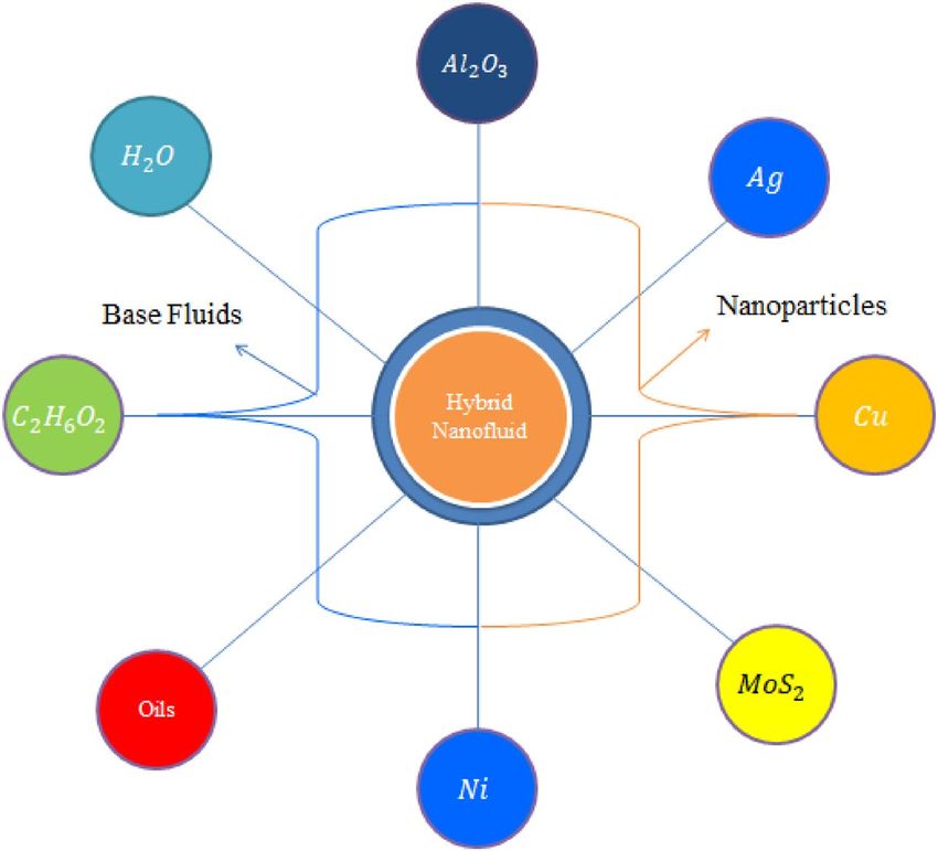
flow transport phenomena are illustrated by Fig. 1. The sketching view of hybrid nanoparticles is considered
by Fig. 2. Thermal properties of hybrid nanoparticles is mentioned in table 1. The non-linear PDEs32,33 are
developed using BLAs (boundary layer approximations) and present flow phenomena in mathematical mode
is established as
∂(xu) ∂(xv)
+ = 0, (1)
∂x ∂z
Scientific Reports | (2021) 11:19604 | https://doi.org/10.1038/s41598-021-99116-z 3
Vol.:(0123456789)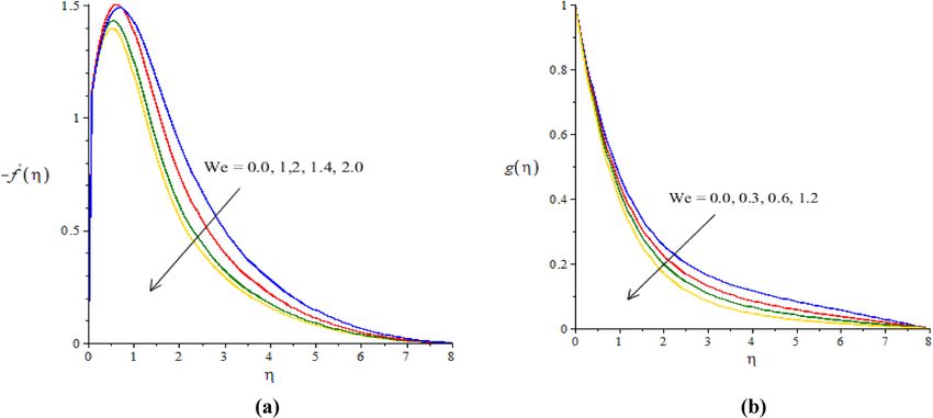
www.nature.com/scientificreports/

                                            Figure 1.  Flow behavior of hybrid nanoparticles.

                                             MoS2 /SiO2                   C2 H6 O2                 MoS2
                                             ρMoS2 /SiO2 = 5060          ρC2 H6 O2 = 1113.5        ρMoS2 = 2650

                                              Cp MoS /SiO = 397.746       Cp C H O = 2430           Cp MoS = 730
                                                     2    2                    2   6   2                  2
                                             kMoS2 /SiO2 = 34.5           kC2 H6 O2 = 0.253        kMoS2 = 1.5
                                             σMoS2 /SiO2 = 1 × 10⁻¹⁸      σC2 H6 O2 = 4.3 × 10⁻⁵   σMoS2 = 0.0005

                                            Table 1.  Thermal properties of hybrid nanoparticles with base fluid.

                                            Figure 2.  The sketching behavior of hybrid nanoparticles.

          Scientific Reports |   (2021) 11:19604 |                     https://doi.org/10.1038/s41598-021-99116-z   4

Vol:.(1234567890)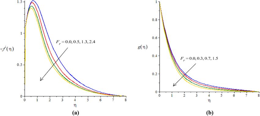
www.nature.com/scientificreports/
v2
�
∂2u
� n−1 � 2 � ∂u �d �
u ∂u ∂u
∂x + w ∂z = x + νhnf ∂z 2
+ Ŵd d (d + 1) ∂∂zu2 ∂z + Gβ(T − T∞ )cosα
B02 σhnf νhnf Fs
, (2)
+ρ 2 2 [vβe − (1 + βe βi )u] − k∗ Fs u − u2
hnf [(1+βe βi ) +βe ] (k∗ )1/2
uv
�
∂2v
� n−1 � 2 � ∂v �d �
∂v
u ∂x + w ∂v
∂z = x + νhnf ∂z 2
+ Ŵd d (d + 1) ∂∂zv2 ∂z
B02 σhnf νhnf Fs (3)
−ρ [uβe + (1 + βe βi )v] − k∗ Fs v − v2
hnf [(1+βe βi )2 +βe2 ] (k∗ )1/2
khnf 3
σ ∗ 16T∞ B02 σhnf
� 2 �
∂ T ∂2T
u ∂T ∂T
� 2 2
�
∂x + w ∂z = + +
(ρcp )hnf ∂z 2 � 3k∗ ∂z 2 ��ρhnf [(1+βe βi )2 +βe2�] u + v
µ
� �
∂u d d ∂u 2 2 (4)
+ (ρChnf) 1 + (Ŵ)d n−1 + ∂v + ∂v
� � � � � � � � � �
d ∂z ∂z ∂z ∂z + Q0 (T − T∞ )
p hnf
The BCs (boundary conditions)32 are simulated using concept of no-slip theory
u = 0, v = �xsinα, T = Tw , w = 0 at z = 0
u → 0, v → 0, T → T∞ at z → ∞
. (5)
The change of variables are constructed as
�1
u = − �xsinα ′ , v = �xsinαg, w = �ν sinα 2 f
�
2 f f
�
x(T0 −T∞ ) . (6)
θ = TT−T
w −T
∞
∞
, η = z �sinα
ν f
, Tw = T∞ + l
The correlations of thermo-physical properties in nano and hybrid nanoparticles are
� � ��
ρnf = (1 − φ)ρf + φρs , ρhnf = (1 − φ2 ) (1 − φ1 )ρ�f + φ1 ρs1� + φ2 ρs2
� � � � � � � � � � � � ��
ρCp nf = (1 − φ) ρCp f + φ ρCp s , ρCp hnf = (1 − φ2 ) (1 − φ1 ) ρCp f + φ1 ρCp s ,
� � 1
+φ1 ρCp s
2
(7)
� � ��
µf µf knf ks +(n+1)kf −(n−1)φ kf −ks
µnf = , µnf = (1−φ )2.5 (1−φ )2.5 , kf =
(1−φ)2.5
� �
ks +(n−1)kf +φ kf −ks
2 1
� � ��
khnf ks2 +(n−1)kbf −(n−1)φ2 kbf −ks2
� �
σhnf 3(σ −1)φ
kbf = �
k +(n−1)kbf −φ2 kbf −ks2
� , σ = 1 + (σ +2)−(σ −1)φ (8)
� s2 � �� � f � ��
σhnf σs2 +2σf −2φ2 σbf −σs2 σbf σs1 +2σf −2φ1 σf −σs1
= � , =
� � �
σf σs2 +2σf +φ2 σbf −σs2 σf σs1 +2σf +φ1 σf −σs1
Equations (1–5) are transformed into dimensionless Eqs. (7–9) using Eq. (6)
2 2.5 2.5 �
� � � �
ν 2 �
f ′′′ + νhnff 21 f ′ − ff ′′ − 2g 2 − 2 θ − M (1−φ 1 ) (1−φ2 )
(1+βe βi )2 +βe2
2βe g + (1 + βe βi )f ′
+(We)d (n−1)(d+1) f ′′′ ff ′′ d + ǫf ′ − H F f ′ 2 = 0,
� � � � (9)
d 1 r
f (0) = f ′ (0) = 0, f ′ (∞) = 0,
νf � ′ � M 2 (1−φ1 )2.5 (1−φ2 )2.5 � 1 �
g ′′ +
νhnf gf − fg −
′
(1+βe βi )2 +βe2
− 2 βe f ′ + (1 + βe βi )g
+(We)d (n−1)(d+1)
d
g ′′ g ′ − ǫg − H1 Fr g = 0,
� � � � 2 (10)
d
+g(0) = 1, θ (∞) = 0,
�
4
� ′′ (ρcp )hnf � 1 ′
kf ′ + kf
� (1−φ1 )−2.5 PrEcM 2
� � �
1 ′ 2
� �2 �
1+ 3Nr θ + khnf Pr f θ − f θ 2.5 2
khnf (1−φ2 ) [(1+βe βi ) +βe ] 4 f + g
� (ρcp )f
2 2
kf (11)
� � � ��� � � �
PrEc n−1 d 1 ′′ d
� ′
� d 1 ′′ 2
� ′
� 2 kf
khnf (1−φ1 )2.5 (1−φ2 )2.5
1 + d (We) 4 f + g 4 f + g + khnf Hs Prθ = 0,
θ(0) = 1, θ (∞) = 0
Physical quantities. The dimensionless parameters of present problem are defined as
xl(�sinα)2 g(T0 − Tw )lβcosα B2 σhnf
Ec =
, =
2 , M2 = 0 ,
Cp f (T0 − Tw ) �sinα νf ρf �sinα
µf Cp f Q0 Fs x νf Fs k∗ kf
Pr = , Hs =
, Fr = , ǫ = , Nr = .
(k∗ )1/2 4σ ∗ (T∞ )3
kf sinα� ρCp f �sinα
Shear stresses in view of y- and x-directions are expressed as
Scientific Reports | (2021) 11:19604 | https://doi.org/10.1038/s41598-021-99116-z 5
Vol.:(0123456789)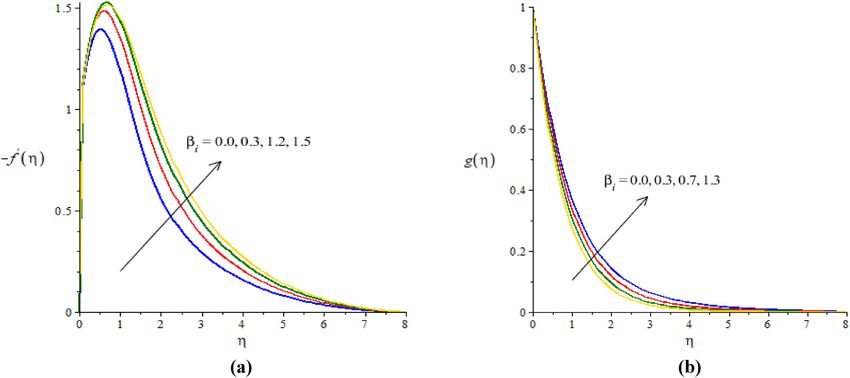
www.nature.com/scientificreports/
2τxz |z=0 2τyz |z=0
Cf = , Cg = ,
ρf (�xsinα)2 ρf (�xsinα)2
1/2 −1 n − 1
′′
d ′′
(Re) Cf = 1+ Wef (0) f (0),
(1 − φ1 )2.5 (1 − φ2 )2.5 d
−1 n − 1
d ′
(Re)1/2 Cg = 1 + Weg ′
(0) g (0).
(1 − φ1 )2.5 (1 − φ2 )2.5 d
The Nusselt number is constructed as
xQw ∂T
Nu = , Qw = −khnf ,
kf (T − T∞ ) ∂z
−khnf ′
(Re)−1/2 Nu = θ (0).
kf
x 2 �sinα
The local Reynolds number is Re = νf .
Numerical method for solution
Weighted
′
residual Galerkin approach (WRGA) is implemented to simulate numerical values of Eqs. (9–11).
Here, f = F is considered to formulate the required residuals. The following description is discussed below.
Division of problem domain. The domain of the problem is broken into 300 elements whereas weak
forms are developed using the weighted residual integrals. Linear polynomial is made over each 300 elements
of domain. Weights functions are multiplied along with residuals and integration is taken. The approximation
computations of f , θ and F are defined below. So the weighted residuals described in24,25,30,31,34 are
ηe+1
′
We f − F dη = 0,
ηe
� �
νf 1 2 ′ 2
F ′′ +
νhnf 2 (F) − fF − 2g − 2 θ
� ηe+1 2 2.5
M (1−φ1 ) (1−φ2 ) 2.5
w1 dη = 0,
� �
− (1+βe βi )2 +βe2 2βe g + (1 + βe βi )F
ηe � �d
+(We)d (n−1)(d+1)
d F ′′ F ′ + ǫF − H1 Fr (F)2
� � � �d
νf′ ′ + (We)d (n−1)(d+1) g ′′ g ′
� ηe+1 g ′′ + gf
νhnf − fg d − ǫg
w2 � ′ �2 dη = 0,
ηe M 2 (1−φ1 )2.5 (1−φ2 )2.5 � 1 ′
�
− (1+β β )2 +β 2 − 2 βe f + (1 + βe βi )g − H1 Fr f
e i e
� ′ � � �d
νf ′ g ′ + (We)d (n−1)(d+1) g ′′ g ′
ηe+1 g ′′ + gf − f − ǫg
�
ν hnf d
w3 dη = 0,
M 2 (1−φ1 )2.5 (1−φ2 )2.5 � 1
− 2 βe F + (1 + βe βi )g − H1 Fr (F)2
�
ηe − (1+β β )2 +β 2
e i e
kf(ρcp )hnf � 1 ′
�
k
(1 + ǫθ)θ ′′ + khnf Pr
(ρcp )f � 2 Fθ − f θ + khnff Hs Prθ
ηe+1
� �
� ′ �2
k
w4 PrEcM 2 1 2 dη = 0,
+ khnff (1+β 2 2 4 (F) + g
e βi ) +βe
ηe
kf
� � � � � �
PrEc 1
F ′ 2 + g ′′ 2
2.5
khnf (1−φ ) (1−φ ) 2.5 4
1 2
Here, w1 , w2 , w3 and w4 are weight functions. The unknown variables f , F, g and θ are considered as
2
2
2
2
f = fi ψj , F = Fi ψj , θ = θi ψj , g = gi ψj ,
j=1 j=1 j=1 j=1
Assembly development. Assembly procedure plays a vital role for development of boundary vector,
source vector and stiffness matrix. Further, it is used to generate the global stiffness matrix while Picard lineari-
zation approach makes linearization in non-linear equations. Hence, local stiffness elements are
ηe+1
ηe+1
dψj
Kij11 = dη, Kij12 = − ψi ψj dη, Kij13 = 0, Kij14 = 0, bi1 = 0,
ψi
ηe dη ηe
Scientific Reports | (2021) 11:19604 | https://doi.org/10.1038/s41598-021-99116-z 6
Vol:.(1234567890)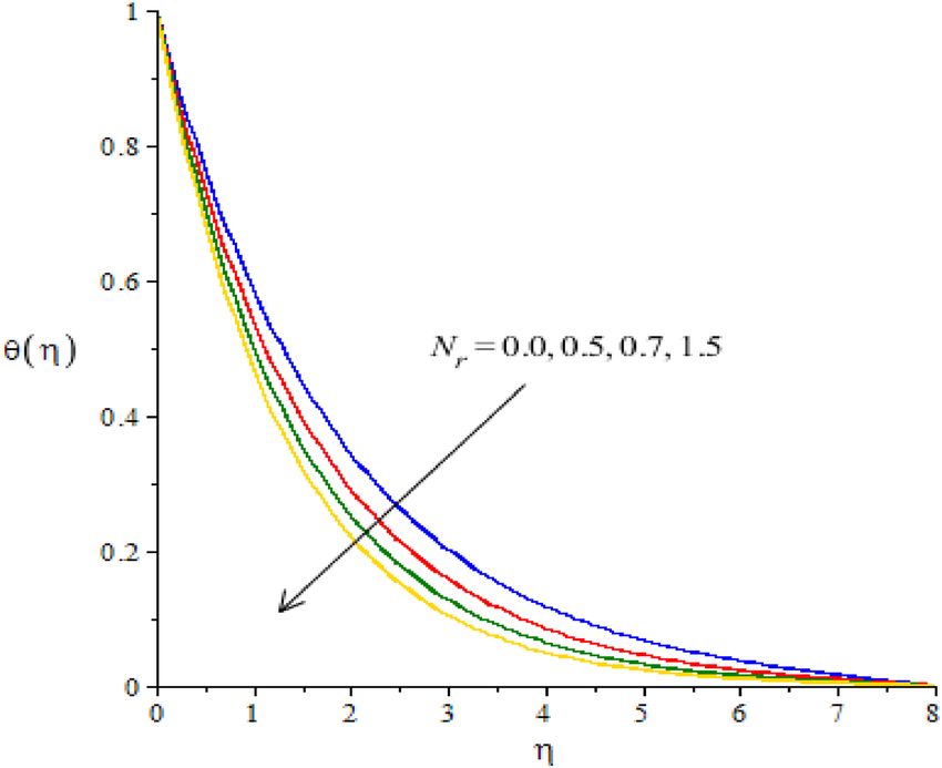
www.nature.com/scientificreports/
ηe+1
M 2 (1 − φ1 )2.5 (1 − φ2 )2.5
Kij21 = 0, Kij23 =
ψj ψi 2g + 2βe ψ i ψ j dη,
ηe (1 + βe βi )2 + βe2
� � �d �
d (n−1)(d+1) ′ dψi dψj
� ηe+1 − 1 + +(We) d F dη dη
Kij22 2 (1−φ )2.5 (1−φ )2.5 �
= M 1 2
� dη,
− (1+β β )2 +β 2 (1 + βe βi )ψj ψi
ηe e i e � �
νf 1 dψj
+ǫψj ψi − H1 Fr Hψj ψi + νhnf 2 Hψj ψi − f ψi dη
ηe+1
νf
Kij24 = 2 ψj ψi dη, bi2 = 0, Kij32 = 0, Kij34 = 0,
−
ηe νhnf
� � �
dψj d dψi dψj
�
d (n−1)(d+1)
� ηe+1 − 1 + (We) d ψ i dη dη dη
Kij33 =− dη, bi3 = 0,
M 2 (1−φ1 )2.5 (1−φ2 )2.5
ηe − 2
(1+βe βi ) +βe2
[(1 + β e βi )]ψ j ψ i − ǫψ j ψ i
−H 1 Fr gψj ψi
ηe+1
M 2 (1 − φ 2.5 2.5
1
1 ) (1 − φ2 )
Kij31 = − 2
βe ψj ψi dη, bi4 = 0,
ηe (1 + βe βi ) + βe2 2
�
dψi j dψ kf (ρcp )hnf � 1 dψj
� ηe+1
−(1 + ǫθ) dη dη + khnf (ρcp )f Pr 2 Fψ j ψ i − f ψ i dη
Kij44 = − dη,
k
ηe + khnff Hs Prψj ψi
ηe+1
kf PrEcM 2 kf −
1 PrEc dψj
Kij41 = − Fψ ψ
j i + F ′
ψ i dη,
ηe khnf (1 + βe βi )2 + βe2 4 khnf (1 − φ1 )2.5 (1 − φ2 )2.5 dη
kf
PrEcM 2 1 ′ dψj
2 g ψj dη
� ηe+1 2
k e βi ) +βe 4
Kij43 =− hnf
k
(1+β
dψi dψj
dη, Kij41 = 0,
PrEc
ηe − khnff (1−φ )2.5 (1−φ2 )2.5 dη dη
1
System of non-linear (algebraic equations) is modeled with help of assembly procedure.
′
f
Mt f , f , θ = Ḟ ,
θ
f
Ḟ (force vector), Mt (global stiffness matrix) and force vector ( Ḟ ) and unknown nodal values .
θ
Convergence analysis. The error is established as
Eer = |χ i − χ i−1 |
and range of convergence is noticed as
Max χ i − χ i−1 < 10−8 .
It is mentioned that system of linear equations is simulated iteratively according computational tolerance
(10−8).
Grid independent investigation. FEM code is designed in Maple 18 while [0, 8] is called computational
domain. Table 2 is performed as grid independent analysis for 300 elements and solution becomes converge at
mid of each 300 elements.
Validation of results. It is noticed that results of present problem is verified with published study by
Malik et al.32 considering Hs = 0, M = 0.002, Fr = 0, ǫ = 0, Ec = 0, Pr = 0.7, βe = 0, βi = 0, φ1 = 0, φ2 = 0.
(Table 3)
Scientific Reports | (2021) 11:19604 | https://doi.org/10.1038/s41598-021-99116-z 7
Vol.:(0123456789)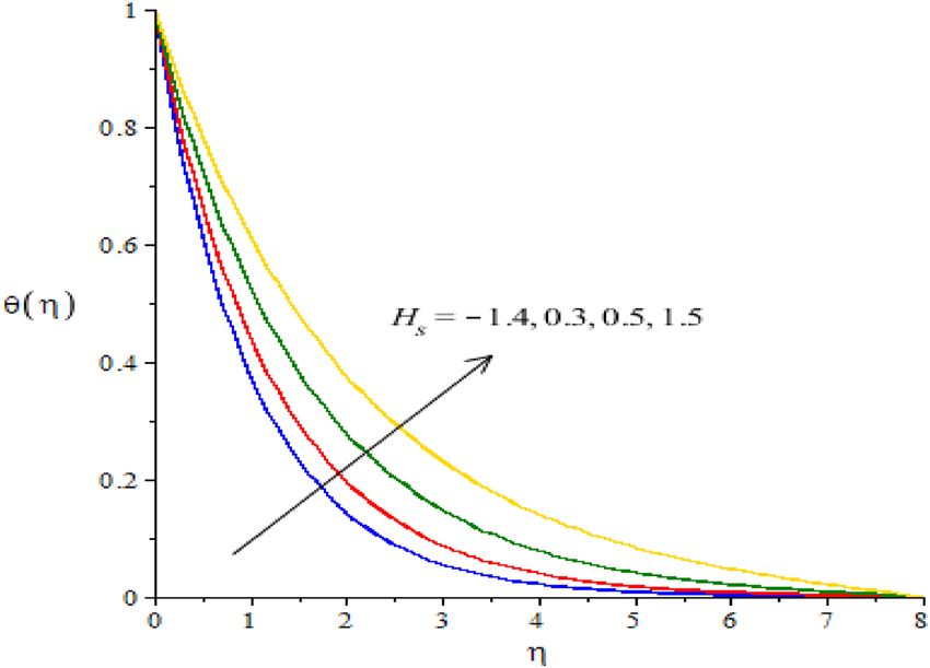
www.nature.com/scientificreports/
Number of elements
η∞
η∞
η∞
f′ 2 g 2 θ 2
30 0.2397335394 0.05453547774 0.1933024653
60 0.2232020794 0.05200805054 0.1819254898
90 0.2177959068 0.05117858942 0.1782491777
120 0.2151131380 0.05076561105 0.1764321953
150 0.2135099778 0.05051829239 0.1753486293
180 0.2124439114 0.05035356891 0.1746289887
210 0.1875839826 0.04551373254 0.1595173162
240 0.2111142682 0.05014775377 0.1737326708
270 0.2106720780 0.05007924754 0.1734348231
300 0.2103180036 0.05002488541 0.1731961042
Table 2. Mesh-free simulations of velocities and temperature via 300 e lements34.
Malik et al.32 present numerical values
(Re)1/2 Cf (Re)1/2 Cg (Re)−1/2 Nu (Re)1/2 Cf (Re)1/2 Cg (Re)−1/2 Nu
0.0 1.0253 0.6153 0.4295 1.0248 0.6149 0.4291
1 2.2007 0.8492 0.6121 2.2003 0.8381 0.6130
10 8.5041 1.3990 1.0097 8.5039 1.3973 1.0088
Table 3. Validation of present results for skin friction coefficients and temperature gradient.
Figure 3. (a, b) The graphical view of velocities versus We.
Results and discussion
In this section, the characterizations of heat transport phenomena in Carreau Yasuda liquid carrying nanopar-
ticles and hybrid nanoparticles over a porous heated cone. The transport of heat energy takes place in terms
of thermal radiation and viscous dissipation under the action of ion slip and Hall forces. The strong technique
is used to capture the results in terms of tables and graphs. The detail study of current model is addressed as:
Graphical simulations of fluid motion. The flow situation is verified against the variation of We (Weis-
senberg number), ion slip and Hall parameters (βi , βe ) and Forchheimer number (Fr ) by Figs. 3a,b, 4a,b, 5a,b,
6a,b. The role of We on the fluid motion is visualized by Fig. 3a,b. The decreasing function is investigated
between the relation of We and motion of fluid particles. This decreasing function is plotted using the concept
of Weissenberg number carrying the study of nanoparticles and hybrid nanoparticles. Physically, Weissenberg
number has direct relation versus elastic force whereas Weissenberg number has inverse relation against vis-
cous force. An increment in Weissenberg number creates more viscosity in fluid particles. More viscous fluid
Scientific Reports | (2021) 11:19604 | https://doi.org/10.1038/s41598-021-99116-z 8
Vol:.(1234567890)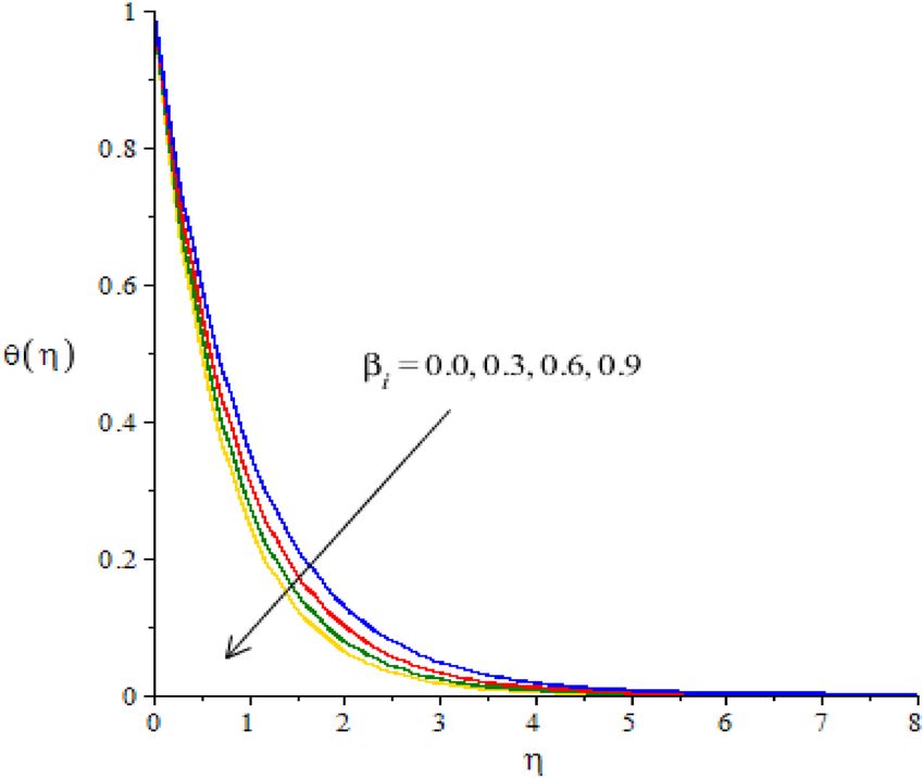
www.nature.com/scientificreports/

                                  Figure 4.  (a,b) The graphical view of velocities versus βi .

                                  Figure 5.  (a,b)The graphical view of velocities versus βe .

                                  is occurred against large values of Weissenberg number. Therefore, reduction in motion of nanoparticles and
                                  hybrid nanoparticles is captured. Figure 4a,b visualize the flow behavior versus the change in ion-slip number. It
                                  is noticed that βi appears in momentum equations reveals the direct relation versus the motion of fluid particles.
                                  An increase in βi results more enhancement in motion of fluid particles is occurred. So, ionization of particles
                                  is useful to develop speed in fluid particles. The concept of ion-slip parameter is formulated using generalized
                                  ohm’s law. The collision due to ions into fluid particles is enhanced when ion-slip number is inclined. Further,
                                  ion-slip number has inverse relation with respect to Lorentz force. So, higher values of ion-slip number create
                                  reduction in Lorentz force. Reduction in Lorentz force makes an increment in motion of fluid particles. Hence,
                                  βi is favorable number to obtain the maximum speed in motion of fluid particles. βe is called Hall parameter and
                                  physical situation is taken out on the flow considering by Fig. 5a,b. Same situation is captured for the case of Hall
                                  parameter towards the motion in fluid particles. In physical point of view, Hall parameter has significant role on
                                  the motion of fluid particles. The fluid motion accelerates versus the impact of βe . It is noticed that inverse rela-
                                  tion is investigated among frictional magnetic force and Hall force. Lorentz force is also reduced versus higher
                                  values of Hall force. Such kinds of happenings are made reason for reduction into fluid motion. The distribution
                                  of Fr on the flow in view of vertical and horizontal directions is addressed by Fig. 6a,b. The primary and second-
                                  ary flows are declined versus the change in Fr . Fr is modeled due to concept of Forchheimer porous media into

Scientific Reports |   (2021) 11:19604 |               https://doi.org/10.1038/s41598-021-99116-z                                                     9

                                                                                                                                                 Vol.:(0123456789)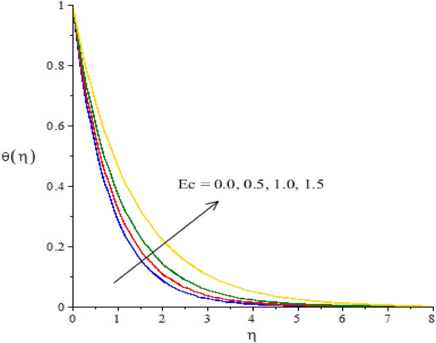
www.nature.com/scientificreports/

                                            Figure 6.  (a,b) The graphical view of velocities versus Fr .

                                            Figure 7.  The graphical view of temperature versus Nr .

                                            fluid particles. Fr is known as non-linear function versus the motion into fluid particles. The retardation force is
                                            formulated against the impact of Fr . This reduction is produced due to porous surface inserting the parameter
                                            Fr . Hence, decreasing trend is captured into the motion of fluid particles.

                                            Graphical simulations of fluid temperature. The phenomenon of fluid temperature is addressed
                                            against the variation of Nr , Hs , βe , βi and Ec. The graphical role of fluid temperature inserting nanoparticles
                                            and hybrid nanoparticles is measured by Figs. 7, 8, 9, 10 and 11. Figure 7 illustrates the behavior of Nr on the
                                            fluid temperature. In this plotting graph, the reduction is simulated in view of thermal energy. This reduction
                                            is created due to large values of thermal radiation number. Physically, heat energy moves away from the sur-
                                            face of cone in form of electromagnetic waves. By this impact, the reduction is occurred into heat energy of
                                            fluid particles. Moreover, inverse relation is modeled among thermal radiation and heat energy. Large values of
                                            thermal radiation number make reduction in heat energy of hybrid nanoparticles. The character of Hs versus
                                            the temperature profile is considered by Fig. 8. The large values of heat energy make the more production in
                                            heat energy while large amount of heat energy is made due to external heat source. Hence, external heat source
                                            makes the reason for obtaining the maximum production of heat energy. It is noticed that negative values of Hs

          Scientific Reports |   (2021) 11:19604 |               https://doi.org/10.1038/s41598-021-99116-z                                                  10

Vol:.(1234567890)
www.nature.com/scientificreports/
Figure 8. The graphical view of temperature versus Hs .
Figure 9. The graphical view of temperature versus βi .
are taken due to heat absorption while positive values for Hs are indicated as concept of heat generation. More
heat energy generates using the concept of external heat source. Figures 9 and 10 reveal the relation between
fluid temperature and ion slip and Hall numbers. The production of heat energy is decreased via enlargement
in ion slip and Hall numbers. It is estimated that ion slip and Hall numbers are appeared in energy equation.
Moreover, the inverse relation is captured versus the existence of ion slip and Hall numbers. An increment in
ion slip and Hall numbers brings the reduction in heat energy. It is mentioned that ion slip and Hall currents
are formulated due to concept of Joule heating phenomena (in the attendance of generalized ohm’s theory).
Joule heating phenomena indicates inverse relation against ion slip and Hall currents. Hence, Joule heating is
inclined using higher values of ion slip and Hall currents. MBLT (thickness of momentum boundary layers)
are adjusted by varying values of ion slip and Hall currents. The motion of ions makes reduction in heat energy
due to large values of ion slip and Hall numbers. The characterization of Ec is considered as an essential role for
maximum achievement of thermal energy while this behavior is captured by Fig. 11. From mathematical view,
Scientific Reports | (2021) 11:19604 | https://doi.org/10.1038/s41598-021-99116-z 11
Vol.:(0123456789)www.nature.com/scientificreports/
Figure 10. The graphical view of temperature versus βe .
Figure 11. The graphical view of temperature versus Ec.
Ec is appeared in energy equation (dimensionless). Hence, direct relation is investigated versus thermal energy.
Physically, Ec is modeled due to viscous dissipation in energy equation. More viscous dissipation is developed
inserting the role of Ec . Heat energy dissipates when viscous nature is occurred into fluid particles. Maximum
heat energy is produced because of additional retarding force. Meanwhile, Ec is visualized as a useful parameter
for developing more thermal energy.
Numerical treatment of surface force and Nusselt number. The surface force, temperature gradient
and Sherwood number are visualized near the surface of cone. The numerical simulations of surface force, Nus-
selt number and rate of solute against change in We, Fr , βe , βi and Hs are simulated. These numerical simulations
are taken out by Table 4. The surface force is decreased via enlargement of heat generation, ion slip and Hall
numbers but surface force called the skin friction coefficient is significantly enhanced considering variation of
Fr . The production of rate of heat energy is increased versus the enhancement of Forchheimer, ion slip and Hall
numbers. Therefore, Forchheimer, ion slip and Hall numbers play a vital impact for the enhancement of tem-
Scientific Reports | (2021) 11:19604 | https://doi.org/10.1038/s41598-021-99116-z 12
Vol:.(1234567890)www.nature.com/scientificreports/
−(Re)1/2 Cf −(Re)1/2 Cg −(Re)−1/2 Nu
0.0 0.4998714299 0.6029282911 0.7104807445
We 0.3 0.8581100631 0.8821689645 0.7114238688
0.5 2.698548989 0.9686090229 0.7121467218
0.0 0.2864470301 0.7360866944 0.7111316028
Fr 0.7 0.2704802904 0.8166854253 0.7098459854
1.3 0.2277144057 0.8787076034 0.7080141595
0.0 0.2713783769 0.1613967311 0.7119591618
βe 0.3 0.2680990013 0.13730063316 0.8132986239
0.7 0.2398120967 0.02406085455 0.9137297415
0.0 0.2753085726 0.2499991558 0.7122827047
0.4 0.1787392657 0.1207572825 0.8099581562
βi
0.8 0.0824121081 0.0860598593 0.9398457277
− 1.3 0.2826682046 0.7000830123 0.17668466241
0.0 0.1839467002 0.5539122359 0.36947614874
Hs
1.2 0.00849283892 0.3058238772 0.71907271478
Table 4. Numerical values of gradient temperature and skin friction coefficients versus various parameters.
perature gradient. In case of heat generation number gradient temperature is reduced due to inserting the large
values of heat generation number.
Key consequences of current model
The porous and rotating cone is used to visualize the impacts of ion slip and Hall forces in thermal energy
mechanism considering Carreau Yasuda liquid. The phenomenon of heat transport is occurred in the presence
of heat generation, nanoparticles, hybrid nanoparticles and thermal radiation. The numerical scheme (FEM) is
used to simulate the numerical results. The prime consequences discussed below.
• Hall and ion slip parameters are considered significant parameters to produce the enhancement in motion of
fluid particles but speed of nano and hybrid nanoparticles becomes slow down versus large values of Forch-
heimer and Weissenberg numbers;
• An enhancement in production of heat energy is addressed via large values of heat generation number and
Eckert number while reduction in heat energy is occurred due to positive values of thermal radiation and
Hall and ion slip parameters;
• The convergence analysis is simulated via 300 elements;
• The temperature gradient is enhanced against the enhancement in Forchheimer, ion slip and Hall parameters
but reverse behavior in noticed for the case of heat generation number;
• Surface force is improved neat wall of cone with respect to variation in Forchheimer number. Surface force
is declined via higher values of heat generation and ion slip and Hall parameters;
• Dimensionless stresses and heat transfer coefficient varies directly against Weissenberg parameter.
Data availability
The datasets generated/produced during and/or analyzed during the current study/research are available from
the corresponding author on reasonable request.
Received: 30 June 2021; Accepted: 13 September 2021
References
1. Mahmood, R. et al. A comprehensive finite element examination of Carreau Yasuda fluid model in a lid driven cavity and channel
with obstacle by way of kinetic energy and drag and lift coefficient measurements. J. Market. Res. 9(2), 1785–1800 (2020).
2. Boyd, J., Buick, J. M. & Green, S. Analysis of the Casson and Carreau-Yasuda non-Newtonian blood models in steady and oscil-
latory flows using the lattice Boltzmann method. Phys. Fluids 19(9), 103 (2007).
3. Coclite, A., Coclite, G. M. & De Tommasi, D. Capsules rheology in Carreau-Yasuda Fluids. Nanomaterials 10(11), 2190 (2020).
4. Pinarbasi, A. H. M. E. T. & Liakopoulos, A. Stability of two-layer poiseuille flow of Carreau-Yasuda and Bingham-like fluids. J.
Nonnewton. Fluid Mech. 57(2–3), 227–241 (1995).
5. Waqas, H., Khan, S. U., Bhatti, M. M. & Imran, M. Significance of bioconvection in chemical reactive flow of magnetized Carreau-
Yasuda nanofluid with thermal radiation and second-order slip. J. Therm. Anal. Calorim. 140(3), 1293–1306 (2020).
6. Hayat, T., Ullah, S., Khan, M. I. & Alsaedi, A. On framing potential features of SWCNTs and MWCNTs in mixed convective flow.
Results Phys. 8, 357–364 (2018).
7. Nayak, M. K., Shaw, S. & Chamkha, A. J. 3D MHD free convective stretched flow of a radiative nanofluid inspired by variable
magnetic field. Arab. J. Sci. Eng. 44(2), 1269–1282 (2019).
8. Hady, F. M., Eid, M. R. & Ahmed, M. A. A nanofluid flow in a non-linear stretching surface saturated in a porous medium with
yield stress effect. Appl Math Inf Sci Lett 2(2), 43–51 (2014).
Scientific Reports | (2021) 11:19604 | https://doi.org/10.1038/s41598-021-99116-z 13
Vol.:(0123456789)www.nature.com/scientificreports/
9. Shafique, Z., Mustafa, M. & Mushtaq, A. Boundary layer flow of Maxwell fluid in rotating frame with binary chemical reaction
and activation energy. Results Phys. 6, 627–633 (2016).
10. Rehman, A. U., Mehmood, R., Nadeem, S., Akbar, N. S. & Motsa, S. S. Effects of single and multi-walled carbon nano tubes on
water and engine oil based rotating fluids with internal heating. Adv. Powder Technol. 28(9), 1991–2002 (2017).
11. Seth, G. S., Mishra, M. K. & Tripathi, R. Modeling and analysis of mixed convection stagnation point flow of nanofluid towards a
stretching surface: OHAM and FEM approach. Comput. Appl. Math. 37(4), 4081–4103 (2018).
12. Kandasamy, R., Mohamad, R. & Ismoen, M. Impact of chemical reaction on Cu, A l2O3 and SWCNTs–nanofluid flow under slip
conditions. Eng. Sci. Technol. Int. J. 19(2), 700–709 (2016).
13. McCash, L. B., Akhtar, S., Nadeem, S., Saleem, S. & Issakhov, A. Viscous flow between two sinusoidally deforming curved concentric
tubes: advances in endoscopy. Sci. Rep. 11(1), 1–8 (2021).
14. Zidan, A. M. et al. Entropy generation for the blood flow in an artery with multiple stenosis having a catheter. Alex. Eng. J. 60(6),
5741–5748 (2021).
15. Saleem, A., Akhtar, S., & Nadeem, S. Bio-mathematical analysis of electro-osmotically modulated hemodynamic blood flow inside
a symmetric and nonsymmetric stenosed artery with joule heating. Int. J. Biomath. 2150071 (2021)
16. McCash, L. B., Akhtar, S., Nadeem, S. & Saleem, S. Entropy analysis of the peristaltic flow of hybrid nanofluid inside an elliptic
duct with sinusoidally advancing boundaries. Entropy 23(6), 732 (2021).
17. Rehman, A., Hussain, A. & Nadeem, S. Assisting and opposing stagnation point pseudoplastic nano liquid flow towards a flexible
Riga sheet: a computational approach. Math. Probl. Eng. 2021, 6610332. https://doi.org/10.1155/2021/6610332 (2021).
18. Akhtar, S., McCash, L. B., Nadeem, S., Saleem, S. & Issakhov, A. Convective heat transfer for peristaltic flow of SWCNT inside a
sinusoidal elliptic duct. Sci. Prog. 104(2), 00368504211023683 (2021).
19. Rizwana, R., Hussain, A. & Nadeem, S. Mix convection non-boundary layer flow of unsteady MHD oblique stagnation point flow
of nanofluid. Int. Commun. Heat Mass Transf. 124, 105285 (2021).
20. Yasin, A., Ullah, N., Saleem, S., Nadeem, S. & Al-Zubaidi, A. Impact of uniform and non-uniform heated rods on free convective
flow inside a porous enclosure: finite element analysis. Phys. Scr. 96(8), 085203 (2021).
21. Ahmad, S., Nadeem, S. & Khan, M. N. Mixed convection hybridized micropolar nanofluid with triple stratification and Cattaneo-
Christov heat flux model. Phys. Scr. 96(7), 075205 (2021).
22. Yasin, A., Ullah, N., Nadeem, S. & Saleem, S. Finite element simulation for free convective flow in an adiabatic enclosure: Study
of Lorentz forces and partially thermal walls. Case Studies in Thermal Engineering, 25, p.100981 (2021).
23. Hussain, A. et al. A combined convection carreau–yasuda nanofluid model over a convective heated surface near a stagnation
point: a numerical study. Math. Probl. Eng. 2021, 6665743. https://doi.org/10.1155/2021/6665743 (2021).
24. Nazir, U., Sadiq, M. A. & Nawaz, M. Non-Fourier thermal and mass transport in hybridnano-Williamson fluid under chemical
reaction in Forchheimer porous medium. Int. Commun. Heat Mass Transf. (2021).
25. Nazir, U., Saleem, S., Nawaz, M. & Alderremy, A. A. Three-dimensional heat transfer in nonlinear flow: a FEM computational
approach. J. Therm. Anal. Calorim. 140(5), 2519–2528 (2020).
26. Abdelsalam, S. I. & Sohail, M. Numerical approach of variable thermophysical features of dissipated viscous nanofluid comprising
gyrotactic micro-organisms. Pramana: J. Phys. 94(1), 1–12 (2020).
27. Sohail, M. et al. Computational exploration for radiative flow of Sutterby nanofluid with variable temperature-dependent thermal
conductivity and diffusion coefficient. Open Physics 18(1), 1073–1083 (2020).
28. Bilal, S., Sohail, M. & Naz, R. Heat transport in the convective Casson fluid flow with homogeneous-heterogeneous reactions in
Darcy-Forchheimer medium. Multidiscip. Model. Mater. Struct. 15(6), 1170–1189 (2019).
29. Sohail, M. et al. Utilization of updated version of heat flux model for the radiative flow of a non-Newtonian material under Joule
heating: OHAM application. Open Phys. 19(1), 100–110 (2021).
30. Nazir, U., Saleem, S., Nawaz, M., Sadiq, M. A. & Alderremy, A. A. Study of transport phenomenon in Carreau fluid using Cattaneo-
Christov heat flux model with temperature dependent diffusion coefficients. Phys. A: Stat. Mech. Appl. 554, 1239921 (2020).
31. Abdelmalek, Z., Nazir, U., Nawaz, M., Alebraheem, J. & Elmoasry, A. Double diffusion in Carreau liquid suspended with hybrid
nanoparticles in the presence of heat generation and chemical reaction. Int. Commun. Heat Mass Transf. 119, 104932 (2020).
32. Malik, M. Y. et al. Mixed convection dissipative viscous fluid flow over a rotating cone by way of variable viscosity and thermal
conductivity. Results in physics 6, 1126–1135 (2016).
33. Saleem, S. & Nadeem, S. Theoretical analysis of slip flow on a rotating cone with viscous dissipation effects. J. Hydrodyn. Ser. B
27(4), 616–623 (2015).
34. Nazir, U., Nawaz, M. & Alharbi, S. O. Thermal performance of magnetohydrodynamic complex fluid using nano and hybrid
nanoparticles. Phys. A Stat. Mech. Appl. 553, 124 (2020).
Acknowledgements
The authors acknowledge the financial support provided by the Center of Excellence in Theoretical and Com-
putational Science (TaCS-CoE), KMUTT.
Author contributions
(1) U.N. and M.S. developed the model and write up the modelling section. (2) Solution methodology section
is updated by U.N. (3) U.N. and M.M.S. draw the graphs. (4) Introduction section is updated by M.M.S., H.A.
and P.K. in the revised draft. (5) H.A. and P.K. confirms the modelling and helped in the literature survey. (6)
Results and discussion section is improved by M.S., M.M.S. and H.A. (7) M.M.S. and P.K. wrote the discussion
section of the revised article. (8) Conclusion section is updated by M.S., H.A. and P.K.
Competing interests
The authors declare no competing interests.
Additional information
Correspondence and requests for materials should be addressed to M.S. or P.K.
Reprints and permissions information is available at www.nature.com/reprints.
Publisher’s note Springer Nature remains neutral with regard to jurisdictional claims in published maps and
institutional affiliations.
Scientific Reports | (2021) 11:19604 | https://doi.org/10.1038/s41598-021-99116-z 14
Vol:.(1234567890)www.nature.com/scientificreports/
Open Access This article is licensed under a Creative Commons Attribution 4.0 International
License, which permits use, sharing, adaptation, distribution and reproduction in any medium or
format, as long as you give appropriate credit to the original author(s) and the source, provide a link to the
Creative Commons licence, and indicate if changes were made. The images or other third party material in this
article are included in the article’s Creative Commons licence, unless indicated otherwise in a credit line to the
material. If material is not included in the article’s Creative Commons licence and your intended use is not
permitted by statutory regulation or exceeds the permitted use, you will need to obtain permission directly from
the copyright holder. To view a copy of this licence, visit http://creativecommons.org/licenses/by/4.0/.
© The Author(s) 2021
Scientific Reports | (2021) 11:19604 | https://doi.org/10.1038/s41598-021-99116-z 15
Vol.:(0123456789)You can also read