Application of Vector Sensor for Underwater Acoustic Communications
←
→
Page content transcription
If your browser does not render page correctly, please read the page content below
Application of Vector Sensor for Underwater
arXiv:1804.06666v1 [eess.SP] 18 Apr 2018

                                                    Acoustic Communications
                                              Farheen Fauziya1 , Brejesh Lall1,2 and Monika Agrawal1,3
                                                   1#
                                                      Bharti School of Telecomm. Techn. and Mgmt.
                                                         2#
                                                            Department of Electrical Engineering
                                                      3#
                                                         Centre for Applied Research in Electronics
                                                          Indian Institute of Technology – Delhi
                                                                 New Delhi, India 110016
                                           Emails: bsz148360@dbst.iitd.ac.in, brejesh@ee.iitd.ac.in, maggarwal@care.iitd.ac.in
                                                                         April 19, 2018

                                                                              Abstract
                                                   The use of vector sensors as receivers for Underwater Acoustic
                                               Communications systems is gaining popularity. It has become impor-
                                               tant to obtain performance measures for such communication systems
                                               to quantify their efficacy. The fundamental advantage of using a vector
                                               sensor as a receiver is that a single sensor is able to provide diversity
                                               gains offered by MIMO systems. In a recent work novel framework
                                               for evaluating capacity of underwater channel was proposed. The ap-
                                               proach is based on modeling the channel as a set of paths along which
                                               the signal arrives at the receiver with different Angles of Arrival. In
                                               this work, we build on that framework to provide a bound on the
                                               achievable capacity of such a system. The analytical bounds have
                                               been compared against simulation results for a vector sensor based
                                               SIMO underwater communications system. The channel parameters
                                               are modeled by analysing the statistics generated with Bellhop simu-
                                               lation tool. This representation of the channel is flexible and allows
                                               for characterizing channels at different geographical locations and at
                                               different time instances. This characterization in terms of channel pa-

                                                                                  1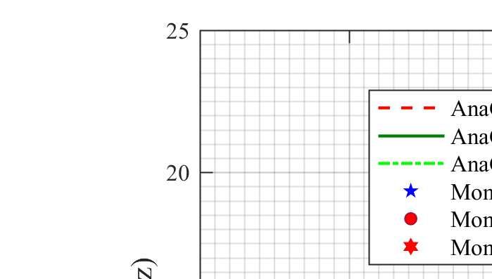
rameters enables the computing of the performance measure (channel
     capacity bound) for different geographical locations.

1    Introduction
With the development of vector sensors for underwater acoustic communi-
cations there has arisen a need to obtain performance measures for such
communications systems. The ability of a single vector sensor to provide
diversity gains has been demonstrated in some recent works [2, 18]. But how
effective is the diversity that a single vector sensor can provide? Researchers
have made some attempts to answer this question by estimating the capacity
of these communications system. This is however an arduous task since the
underwater channel is very complex and difficult to model [4, 25]. A large
volume of research with multicarrier transmission in the form of OFDM is
done to overcome the inter-symbol interference resulting from the frequency
selectivity of underwater acoustic communication channel [3, 21]. In [3], or-
thogonal frequency division multiplexing (OFDM) is taken into account with
cooperative transmission to improve the performance and to take advantage
from the spatial diversity. Besides, the channel is very topography specific
i.e. has strong dependence on the location. A recent attempt has been made
to develop an AoA based framework for representing the shallow underwater
channel [8]. This framework is simple and intuitive and can easily be adapted
to represent different channel behaviors. In this work, we use that framework
to obtain an upper bound on capacity of the underwater channel. A tight
upper bound has been obtained in this work.
     Work on capacity computation of MIMO channels in underwater com-
munications has been reported in [6, 12]. However, all these work consider
MIMO implemented using an array of scalar sensors. Radosevic et.al. [22] use
probe signals to estimate the statistical properties of the time varying chan-
nel. They show that Rician fading is a good match for experimental data.
This model is used to evaluate the channel capacity for both the Single Input
Single Output (SISO) and MIMO systems. In another work [14], the authors
obtain a lower bound on achievable information rate for MIMO communica-
tions over underwater acoustics channels. They evaluate the ergodic capacity
for partial channel state information (CSI) at the transmitter and no CSI at
the transmitter scenarios. That work also uses an array of scalar sensors
to achieve MIMO capability in underwater acoustic communication systems.

                                      2
Little work is available on channel capacity computation for vector sensor
based underwater MIMO communications. One work that does attempt this
is by Abdi el.at. [9, 10]. That work assumes that the number of transmit-
ters is large. This is not a realistic assumption when one is attempting to
compute the MIMO capacity of communications system, which consists of a
single scalar transmitter and a single vector receiver. Besides, in that work
different capacity expressions have been obtained for low SNR and high SNR
scenarios. Finally, the normalization performed on the correlation matrix for
the vector sensor case is not entirely justified. However, the work provides a
first approach for computing the maximum data rates of the particle velocity
channels. In [8], the authors present an AoA framework for computing the
underwater channel capacity. We exploit that framework to obtain capacity
bounds that are not restricted by the simplifying assumptions used in that
work.
It is well known that acoustic shallow water channel is very complex
and location specific. Numerous efforts have been made to come up with
good propagation models which can be used for generating simulated data
for different underwater acoustic channel scenarios. Some of the models are
based on Ray theory, while others use model expansions and wave number
techniques. Models are classified as either being range dependent or range
independent. In a range dependent model, the environmental parameters
like water depth, sound speed etc are kept fixed with range whereas in range
independent models, the parameters are allowed to vary with distance. Ray
theory is based on simplification applied to the wave equation and can be
viewed as a high frequency approximation of the same. The method is how-
ever reasonably accurate for communication over short and medium range.
In models based on Ray theory, trajectories of rays from source are com-
puted. Ray tracing method have the advantage of being fast, amenable to
incorporating directionality and of being accurate. A very popular Ray the-
ory based model is Bellhop [7, 13], which is used in this work. Beam tracing
is a variant of ray tracing [?]; it applies information about beam width asso-
ciated with each ray to determine amplitude of the pressure, thus overcoming
the shadow zone problems associated with the ray tracing methods. Bellhop
predicts acoustic pressure fields in ocean environments and uses ray theory
to provide an accurate deterministic picture of underwater acoustic channel
for a given geometry and signal frequency. Bellhop provides the flexibility of
simulating different environmental conditions and accept the corresponding
information via the configuration file. The simulation parameter uses in this
3work are shown in Table 2.
To derive the capacity, the following model of the channel has been as-
sumed [8]: The path gains are usually modeled as Rayleigh distributed [17,29]
and we use the same model for path gain. The other aspect of shallow wa-
ter channel is that the path gain is a function of the AoA. This dependence
is analyzed using the Bellhop simulation tool and is incorporated into the
channel model. A tight upper bound is computed based on this model of
underwater channel. The specific contributions of this paper are listed as
follows,
(i) AoA based framework for channel characterization.
(ii) The channel parameters models are obtained.
(iii) Channel capacity bound is obtained.
(iv) The bound is compared to SISO channel capacity. This paper is orga-
nized as follows: This section is the introduction. Sections 2 presents brief
introduction of the acoustic vector sensor, section 3 contains description of
the system model. In section 4 we derive the capacity of vector sensor based
SIMO system. Mathematical description and closed form expression for the
capacity are presented. Section 5 contains the numerical results, and the
conclusions are given in section 6. For enhancing readability of the paper,
the list of symbols is given in Table 1.
Table 1: List of main symbols
s Transmitted Signal
r Scalar component of the received acoustic pressure signal
ry Pressure equivalent velocity component along range
rz Pressure equivalent velocity component along depth
n Ambient noise pressure
ny Pressure equivalent ambient noise velocity component along range
nz Pressure equivalent ambient noise velocity component along range
h Channel impulse response of scalar component of vector sensor
hy Channel impulse response of particle velocity component along range
hz Channel impulse response of particle velocity component along depth
γ, γib , γis Angle of arrival of reflected rays, ith rays reflected from the bottom and ith rays reflected from the surface
hLoS , hib , his Path gain of LoS path, ith path from bottom and ith path from surface
τLoS , τib , τis Path delay of LoS path, ith path from surface and ith path from bottom
Λ, ξ, ς Scaling parameter, Mean value and Spreading factor of scaled Gaussian function
θib , θis , βib , βis Parameters of the AoA pdf
Nc Noise covariance matrix at receiver
E[.] ∗ δ(.) Expectation operator, Convolution operator and Dirac delta function respectively
(.)T & (.)† Transpose and Hermitian operators respectively
42 Acoustic Vector Sensor
Before describing the system model, we present a brief discription of acoustic
vector sensor. An acoustic vector sensor is different from a scalar acoustic
sensor, in that it measures both the acoustic pressure and the acoustic veloc-
ity. This information can be used to estimate the acoustic intensity vector,
which is a measure of the acoustic energy flow rate per unit area in the direc-
tion perpendicular to the flow. Mathematically acoustic intensity vector can
be represented a product of acoustic pressure and acoustic particle velocity.
Vector sensors are usually designed in one of the following two ways: (i)
Pressure-velocity based method resulting in a class of vector sensors called
inertial sensors and (ii) Pressure-pressure based method leading to a class of
vector sensors categorized as gradient sensors.
Inertial sensors work directly on the particle velocity. The particle veloc-
ity can be obtained either by time integration of the accelerometer measure-
ments or by direct measurement of velocity e.g. using a Microflown. Inertial
sensors offer the advantage of broad dynamic range, however, packaging of
the sensor without affecting its response to the motion is a challenge. Also,
such sensors do not distinguish between acoustic waves and non-acoustic
motion (e.g. support structure vibrations) and must, therefore, be properly
shielded from such disturbances.
In gradient sensors, finite difference approximation of the spatial deriva-
tive of the sound-field is used to compute the particle velocity. Such sen-
sor require that the separation d between the two microphones should be
much smaller than the acoustical wavelength, λ. An increase in separation
(for a fixed frequency) leads to an increase in error in the pressure-gradient
estimate. Also, such sensors are sensitive to sensor noise, microphone mis-
match, reflection and diffraction of the source radiated signal, placement of
the microphones, the structure that holds the microphones and the polar
pattern characteristics of each microphone. A typical gradient sensor has
closely spaced omni-directional and/or gradient-microphones that measure
the pressure and pressure-gradients in the three orthogonal directions which
are, in turn, used for particle velocity estimation. In summary, gradient
sensors can be manufactured in smaller sizes and thus are more suitable for
high frequency applications. However, the finite-difference approximation
limits their operating dynamic range. Given their individual advantages and
disadvantages, the choice of type of vector sensor depends on the application.
The output of an AVS consists of four channels, namely, the acoustic
5Range
Sea Surface
Tx Depth
Rx Depth
n
h r
Tx n y
hy
Water Depth
hz ry
Velocity component along range
Rx nz
Velocity component along depth
rz
Sea Bottom
Figure 1: Acoustic vector sensor receiver in underwater communications system.
pressure and the three Cartesian components of the particle velocity. In this
paper the vector sensor considered gives a measure of three components, the
acoustic pressure and two Cartesian components of particle velocity (those
along range and depth).
3 System Model
In this paper, we consider an underwater communications system with a
scalar transmitter and a vector sensor receiver. The system model is shown
in Fig. 1. The received signal consists of a scalar component and two vector
components [1]. To aid in understanding the representation proposed for
the pressure equivalent velocity component along range and depth, a brief
description of the mathematical model for acoustic flow is now presented.
The relation between pressure and particle velocity can be represented as,
∂~v
▽h = ρ (~v .▽)~v + , (1)
∂t
where, ~v is the particle velocity, h is the pressure and ▽ is the Laplace
operator. Using the linearized momentum align the relation between acoustic
6particle velocity and pressure is given as, [16],
∂~v
▽h = −ρ (2)
∂t
Using Eqn. (2), the velocity component along y & z at frequency f can
be represented as follows,
1 ∂h z 1 ∂h
vy = − , v =− (3)
jρω ∂y jρω ∂z
where, ρ is the fluid density, ω = 2πf and j 2 = −1. From Eqn. (3), it is
clear that velocity in a certain direction is directly proportional to the spatial
pressure gradient in that direction. The acoustic pressure channel represents
the scalar channel h and the two particle velocity components represent the
pressure equivalent velocity channels along range and depth denoted by hy
and hz respectively. The pressure equivalent velocity component along range
and depth can be obtained by multiplying velocity channel v y & v z with
the negative of acoustic impedance (−ρc), where c is the speed of sound.
Incorporating the wave number k = ω/c = 2π/λ into the sound, the final
expression for pressure equivalent velocity channel can be written as [1],
1 ∂h z 1 ∂h
hy = −ρcv y = , h = −ρcv z = , (4)
jk ∂y jk ∂z
The received signal components can be viewed as convolution of the trans-
mitted signal with the three channel impulse responses. The pressure com-
ponent of the received signal can be represented as follows,
r = s ∗ h + n. (5)
Similarly received signal components along range and depth can be written
as
r y = s ∗ hy + ny , r z = s ∗ hz + nz , (6)
where, r and s represent received and transmitted signals respectively, hy
is the pressure equivalent velocity component along the range and hz is the
pressure equivalent velocity component along the depth. r y is received signal
component along the y direction (range), r z is received signal component
along z direction (depth), n, ny and nz are the ambient noise pressure and
7Range
Sea Surface
Tx Depth
Rx Depth
Water Depth
Tx
ᶿLoSᶿ1S ᶿ2S
ᶿ1b Rx
ᶿ2b
Sea Bottom
Figure 2: System model based on vector sensor receiver
pressure equivalent ambient noise velocities along range and depth respec-
tively. This communication systems can be represented as a 1 × 3 SIMO.
The channel matrix H is given as follows.
h
H = hy
(7)
hz
Given this system model, we now present brief a description of the statis-
tical properties of the channel and how they have been incorporated in the
channel model. In this work, it has been assumed that the ray will scatter
only from the surface and bottom of the sea. The path gain has been as-
sumed to be Rayliegh distributed and the sacale parameter of the density
function depends on the AoA.
α α2
ph|γ (α|γ) = 2 exp − 2 ; h≥0 (8)
σ (γ) 2σ (γ)
where, γ is the AoA and σ is the scale parameter. At the receiver side,
amplitude will be maximum if the ray comes along the direct path (i.e. with
AoA θLoS ) and as one moves away from LoS the amplitude in either direction
will decrease till it reaches zero at angles ±π/2. To account for this variation
8Figure 3: Dependence of path gain on the Angle of Arrival of the path
in amplitude as a function of AoA, the scale parameter of Rayleigh distribu-
tion σ 2 is modeled as a (scaled Gaussian) function of AoA with maximum
amplitude at θLoS . No studies exist on the distribution of path gain as a
function of AoA. However, studies on distribution of path gain as a function
of time of arrival show the dependence as Gaussian [19, 20]. Drawing inspi-
ration from those works and by performing statistical analysis using data
generated using Bellhop [7], we found that the best fit for the dependence
of path gain on AoA is scaled Gaussian. Given that, the energy correspond-
ing to a Rayliegh distribution is directly proportional to σ 2 we choose the
map between AoA and Rayleigh distribution parameter to be scaled Gaus-
sian. The analysis reveals that the best fit for the path gain statistics (as a
function of AoA) is scaled Gaussian,
γ−ξ 2
σ 2 (γ) = Λe−( ς ) (9)
where, Λ, ξ, & ς corresponds to scale, mean and spreading factor of the
fitted distribution. To illustrate the correctness of the fit, the comparison
between the simulation statistics and the scaled Gaussian curve used to fit
9those statistics is shown in Fig. 3. The figure clearly shows that scaled
Gaussian is a very good approximation of the path loss statistics as a function
of AoA. The goodness of fit has been tested using some popular measures
and the resutls reveal a good fit [19]. The values for SSE, R-square and
RMSE respectively are 8.08e−08 , 0.9334 and 7.215e−05 . These results are for
a fit with 95% confidence bound, which clearly show that the fit is good [19].
Another point to note is that this model for dependence of path gain on
AoA implictly incorporates the effect of bottom reflection coefficients. The
bottom reflection coefficients are a function of the grazing angle [11, 23].
Smaller angles result in higher attenuation and larger angles lead to lower
attenuation. The paths that arrive with high AoA constitute rays that have
grazed the bottom at lower angles and hence have suffered from greater
attenuation. This is reflected in the relatively steep reduction in path gain
as a function of AoA. If this dependence had been ignored the path gain would
have been proportional to the cosine of the AoA, however by including the
effect of bottom reflection coefficients the appropriate fit for the path gain is
scaled Gaussian and not a cosine map. This is borne out by the curve fitting
analysis.
Figure 4: Probabilty density function characterizing the AoA distribution of
the ith path.
The other characteristic of the channel that one needs to model is the
10probability distribution of the AoA, γ of the received path. In our work, the
probability density function is represented using the following equations,
(1
2 (θi + βi − γi ) ; θi < γi < θi + βi
pγi (γi ) = β1i (10)
β2
(γi − θi + βi ) ; θi − βi < γi < θi ,
i
where, γi is the AoA of rays, θi , is the parameters of the probability density
function characterizing the AoA of the ith path. βi is the spread of AoA
about θi . In literature the AoA distributions have been variously modeled.
In their work Abdi et.al. [1] use Gaussian with very small variance to model
the AoA distribution. However, no work categorically assigns a distribution
to the AoA. In wireless communications, researchers have proposed Laplacian
as a distribution of choice [26]. There is however consensus on the fact that
the distribution of the AoA for a path is of a small variance [1, 2]. Further,
it can be shown that Gaussian (as also Laplacian) with small variance can
be modeled using triangular distribtution function [30]. For this reason and
for aiding mathematical tractability we approximate the density funtion of
the AoA as triangular [30].
Given these models for the channel characteristics, we continue our de-
scription of the underwater acoustic communications system. The channel
response can be represented in terms of individual path gains and AoA’s as
follows:
XN
h= hi δ(γ − γi )δ(τ − τi )δ(γ), (11)
i=1
where N is the total number of paths, and as shown in Fig. 2, hi is the path
loss along path i and γi is the AoA of the ith path. Using the framework
introduced in this section,
N
X
hyi = hi cos[γi ]δ(γ)δ(τ − τi ), (12)
i=1
represents the path gain along the range. Similarly path gain along depth
can be represented as
N
X
hzi = hi sin[γi ]δ(γ − π/2)δ(τ − τi ), (13)
i=1
11where, N is the number of paths reaching the receiver after no/single/multiple
reflection/s from the surface and the bottom. For this framework, the prob-
ability density function of the AoA is represented as triangular and the path
loss is modeled using a family of Rayleigh pdfs [23]. The variance of Rayleigh
pdfs is a function of AoA of that path. This dependence is modeled using
a scaled Gaussian function with the max value at θLoS (the angle that LoS
path makes with respect to range). Simulation parameters for Bellhop used
in this analysis are listed in Table 2.
3.1 AoA Representation
The propagation speed varies with water depth and hence in deep water the
acoustic rays bend towards the layer with small propagation speed. However,
in shallow water environment, the propagation occurs with constant speed.
Therefore, the shallow water environment is considered to be an isovelocity
medium (i.e. no refractions only reflections) and acoustic rays travel along
straight lines. However, due to severe multipath effect caused by surface
and bottom reflections, the transmitted signal propagates over large number
of paths in shallow water. The two dimensional channel model for shallow
water environment is bounded by oceans surface and bottom as shown in
Fig. 2.
The received signal in a typical shallow underwater acoustic communica-
tions scenario consist of multiple paths arriving at different time instances.
Given the relatively small speed of an acoustic wave in water and relatively
large range the arrival times are typically displaced by several symbol dura-
tions. Accordingly, the channel response can be represented as Eqn.(11). In
the shallow water scenario, the multiple paths can be attributed to reflec-
tions from the surface or bottom or from both. These reflections imply that
unique AoA is associated with every individual path.
3.2 Channel Modeling
Given the channel representation in Eqn. (11), Eqn. (12) & Eqn. (13) we
now need to apply the model for AoA, γ, and compute the corresponding
path gain, h, to fully characterize the channel. In literature, the path gain
in UWAC systems has been modeled as Rayleigh distributed [12]. However,
in UWAC systems the individual paths arrive along multiple angles and at
multiple time instances. Since the path gain depends on number of reflections
12Figure 5: Impulse response as a function of (a) Delay and (b) AoA for
different ranges
and hence the AoA, this dependence can be incorporated into the distribution
13as follows,
α α2
phi (α) = exp(− ) α≥0 (14)
σi2 (γi ) 2σi2 (γi )
As mentioned earlier, the dependence of scale parameter on the AoA, has
been obtained using statistical analysis of the path gain. Bellhop has been
used to generate path gain and corresponding AoA data. The analysis reveals
that the best map for representing the dependence of the scale parameter on
AoA is scaled Gaussian.
γ−ξ 2
σ 2 (γ) = Λe−( ς ) (15)
The value of Λ, ξ & ς can be heuristically estimated for the particular
shallow water channel where the model is applied. The values used in this
work are given in the Table 2.
The other characteristic of the channel that has been modeled is the
probability density function of the AoA. In literature [24], the AoA has been
variously modeled. Some popular representations include, Von Mises, Lapla-
cian and even Gaussian distribution.
( −(γ−µ)2 /2σ2
Ae √ − π/2 + µ ≤ γ ≤ π/2 + µ,
pγ (γ; µ, σ) = σ 2π (16)
0 otherwise,
√
2|γ−µ|2 /σ
(
Ae− √ − π/2 + µ ≤ γ ≤ π/2 + µ,
pγ (γ; µ, σ) = σ 2 (17)
0 otherwise,
where, Eqn. (16) represents the pdf of Gaussian distribution and Eqn. (17)
represents the Laplacian distribution. The parameter σ controls the spread
of the functions, while the constant A is set such that area under the curve
is one. For shallow water UWAC systems and for typical ranges the AoA
are small and their spread about the mean value is smaller still. This ob-
servation allows us to use simplified pdf to make the performance analysis
mathematically tractable. The approximation given in Eqn. (10) results in
negligible error, however it makes the analysis mathematically tractable [15].
Given this channel characterization, we now derive the channel capacity
in the following sub-section.
144 Channel Capacity
In the previous section, we have described the channel and proposed an AoA
based model for it. In this section, we compute the channel capacity using
the proposed channel characterization. Channel capacity can be computed
in terms of the mutual information between the transmitted and received
signal. The mutual information between the transmitted and received signals
is defined as,
XX p(s, r)
I(S; R) = p(s, r) log (18)
sǫA rǫB
p(s)p(r)
and formally the capacity is defined as,
C = sup I(s; r)
pS (s)
where, sup is supremum.
For the SIMO case with L received antennas, the received signal at the
th
i antenna is,
r (i) (n) = h(i) (n) ∗ s(n) + η (i) (n) for i = 1 to L (19)
where, h(i) (n) is the impulse response corresponding to the ith subchannel.
Here, s(n) is the transmitted signal and η (i) (n) is the noise at the ith receive
antenna.
For the current setting L = 3, corresponding to the scalar sensor and the
two components of the vector sensor, the corresponding signals are,
r = h(n) ∗ s(n) + η(n)
r (y) = hy (n) ∗ s(n) + η y (n) (20)
r (z) = hz (n) ∗ s(n) + η z (n)
From [1], we know that the noise energy corresponding to the three diverse
receive paths is ΩN , Ω2N and Ω2N respectively. Where, ΩN is the variance of
the additive Gaussian noise η. Also these noise components are independent
of each other. The impulse responses h(n) can be represented in the terms
of a vector h, with each entry corresponding to the gain associated with the
different paths of the sub-channels.
15The channel capacity will now be computed by applying the channel
model characterization to Eqn.(20) The ergodic capacity of MIMO commu-
nications system is given as follows [6, 27]:
ρ †
C = E log2 det(I + H H) bits/s/Hz, (21)
Nt
where, I is Nt × Nt identity matrix, ρ is the SNR at the receiver and H is
the Nr × Nt channel matrix. Nt is the number of transmitters and Nr is the
number of receivers. For the SIMO case, the ergodic capacity reduces to the
following forms,
" L
!#
X
(i)
C = E log2 det(I + ρ |h | bits/s/Hz, (22)
i=1
For the vector sensor based SIMO system under consideration the ergodic
capacity is given as follows,
C = E log2 1 + ρE |h|2 + 2|hy |2 + 2|hz |2 ,
(23)
were, h, hy & hz components are multiplied by two because the noise along
these components is half of the noise along the corresponding scalar compo-
nents. Also, as mentioned previously the three noise components are uncor-
related [1]. Obtaining closed form for Eqn. (22) is non trivial [5]. In this
paper, we obtain a bound on capacity and show how the bound compares to
the simulated capacity.
4.1 Bound on Capacity :
As discussed above obtaining closed form expression for capacity is an ardu-
ous task. So in this subsection we obtain an upper bound on capacity. Given
the system representation, we now derive the channel capacity for this SIMO
system.
To overcome the difficulties in obtaining a closed form for the above
equation, we use Jensen’s inequality to obtain the upper bound on capacity.
Jensen’s inequality [28] states that given a random variable x and a convex
function φ,
E {φ(x)} ≤ φE {x} .
16Noting that log2 [. ] is a convex function, the channel capacity bound can be
represented as follows,
C =E log2 1 + ρ(|h|2 + 2 |hy |2 + 2 |hz |2 )
(24)
≤ log2 E 1 + ρ(|h|2 + 2 |hy |2 + 2 |hz |2 ) .
therefore,
2 2 2
CU B = log2 1 + ρE(|h| + 2 |hy | + 2 |hz | ) ]. (25)
The bound has been computed using system model shown in Fig. 2. Here h,
hy and hz can be correlated. To handle this correlation, note that,
N
X N
X
y
h= hi δ(γ − γi )δ(τ − τi ), h = hi cos(γi )δ(γ)δ(τ − τi ),
i=1 i=1
N
X
hz = hi sin(γi )δ(γ − π/2)δ(τ − τi )
i=1
Now,
PN PN
|h|2 = hh† = i=1 |hi |2 , |hy |2 = hy (hy )† = 2 2
i=1 |hi | cos (γi ) and
|hz |2 = hz (hz )† = N 2 2
P
i=1 |hi | sin (γi )
Incorporating this in Eqn.(25), we obtain
" N
!#
X
|hi |2 1 + 2 cos2 (γi ) + 2 sin2 (γi )
CU B = log2 1 + ρEh,γ
i=1
" N
!#
X
2
= log2 1 + 3ρEh,γ |hi |
i=1
" Z Z N
#
X
= log2 1 + 3ρ |hi |2 ph|γ (h)pγ (γ)dhdγ
i=1
" N Z
Z X #
= log2 1 + 3ρ |hi |2 ph|γ (h)dh pγ (γ)dγ (26)
i=1
17Given the ph|γ (h) is Rayleigh distributed,
" Z XN
#
CU B = log2 1 + 3ρ σi2 (γ)pγ (γ)dγ
i=1
" " N Z ##
X
= log2 1 + 3ρ σi2 (γ)pγi (γ)dγ (27)
i=1
we know that σi2 (γ) is scaled Gaussian and pγi (γ) is the triangular distribu-
tion characterizing the AoA of the ith path. Substituting these values and
simplifing we obtain the following form for the upper bound.
N
"
1
2 2 √
− (βi + θi + ξ) − (βi − θi + ξ) θi − ξ
X
2
CU B = log2 1 + 3ρ Λς e + e + π 2(ξ − θ i )erf
i=1 i
β2 ς2 ς2 ς
β i + θi − ξ β i − θi + ξ
+(βi + θi − ξ)erf + (βi − θi + ξ)erf (28)
ς ς
In the next section, we present simulation results for different parameter
values. We also compare the upper bound to the simulated capacity of vector
sensor based UWAC system.
Table 2: Simulation Parameters
Parameters Symbols Value
Range (km) R 1,5,9
Water depth (m) dw 250
Transmitter depth (m) dt 150
Receiver depth (m) dr 130
Sound speed (m/s) c 1520
Frequency (kHz) f 5,12,22
No. of beams Nbeams 9000
3
Water density (kg/m ) ρo 1027
Beam take off angle - -90 to 90
Surface type - Vaccum
Speed at bottom (m/s) cp 1550
Bottom density (g/cm3 ) - 1.8
Bottom attenuation (dB/λ) - 0.6
Ambient Noise power - 1.3 ×10⁻⁸
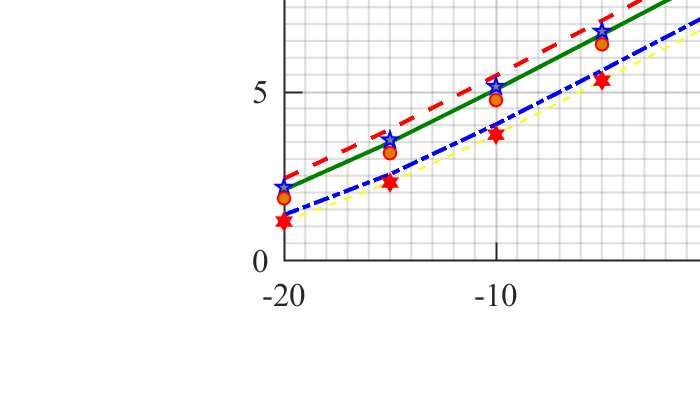
185 Numerical Results and Simulation
In this section, we present the simulation results. The bound on the capacity
obtained in the previous section is now analyzed to see how effective it is as a
measure of performance. We simulate the capacity for vector sensor receiver
case.
The simulation results show that the computed bound is tight and a good
measure of performance of vector sensor based underwater communications
system. We analyze the capacity of such system under different channel
conditions. This study is important because as already stated earlier the
capacity of underwater channel is very location specific. We vary the model
parameters to simulate different channel scenarios and analyze how the ca-
pacity changes as a functions of these parameters.
Analytical capacity for different ranges with different frequency are shown
in Fig. 6. This plot provides a summary of how capacity varies as a function of
these three variables viz, SNR, operating frequency and range. The capacity
as a function of SNR (for a fixed frequency of operation and varying values
of range) is plotted in Fig. 7. The bound on capacity and simulated vector
sensor capacity are plotted. As can be observed, the bound obtained is very
tight. The experiment is repeated to obtain capacity as a function of SNR
range for a fixed frequency and varying values of range refer to Fig. 8. Again
the tightness of the bound can be easily observed.
Further experiments were performed to obtain the capacity as a function
of range and that of the number of scatterers. Fig. 9, clearly shows that
capacity decreases with an increase in frequency of operation. Fig. 12 shows
that as the number of scatterers increases (number of rays impinging on the
receivers increases) the capacity increases and then flattens out. In Fig. 13,
we plot the capacity as a function of frequency (for fixed values of SNR
and number of paths). As the range increases the plots move downwards
indicating a reduction in capacity. For a fixed range the capacity decreases
as a function of frequency and the decrease becomes sharper as the frequency
becomes higher. Finally the plot in Fig. 14 shows that capacity of the SISO
underwater communications system is higher than that of a SISO UWAC
system for all values of SNR.
19Combined Analytical Capacity for NRay=15
30
Analytical Capacity (Range=1km,Freq=5 KHz)
Analytical Capacity (Range=5km,Freq=5 KHz)
Analytical Capacity (Range=9km,Freq=5 KHz)
Analytical Capacity (Range=1km,Freq=12 KHz)
25 Analytical Capacity (Range=5km,Freq=12 KHz)
Analytical Capacity (Range=9km,Freq=12 KHz)
Analytical Capacity (Range=1km,Freq=22 KHz)
Analytical Capacity (Range=5km,Freq=22 KHz)
Analytical Capacity (Range=9km,Freq=22 KHz)
20
Capacity(bits/sec/Hz)
15
10
5
0
-20 -10 0 10 20 30 40 50 60
SNR(dB)
Figure 6: Analytical capacity as a function of SNR for different ranges and
different frequencies
6 Conclusions
In this paper, we derive a tight upper bound on the capacity of a vector
sensor based underwater communications system. An AoA based channel
representation is used to derive the results. First the AoA based framework
is used to derive the density function of path gain. The same is then used
to obtain a closed form expressions for the upper bound of channel capac-
ity. The parameters of the channel have been modeled using the statistics
generated using the Bellhop simulation tool. Extensive experimentation is
performed and the results analyzed to check the efficacy and applicability
of the proposed measure. The capacity under different channel conditions
is obtained and a measure of the efficacy of vector sensor based underwa-
ter communications system is provided. The results derived are expressed
in terms of parameters that represent the specific location of the channel.
20Figure 7: Capacity variation as a function of range for fixed number of rays
(NRay=15) and frequency (f=5kHz)
Thus, the result can easily be tailored for different shallow underwater chan-
nels that one encounters at different geographical locations and at different
temporal instances.
References
[1] A. Abdi and H. Guo. A new compact multichannel receiver for underwa-
ter wireless communication networks. IEEE Transactions on Wireless
Communications, 8(7):3326–3329, July 2009.
[2] A. Abdi and H. Guo. Signal correlation modeling in acoustic vector
sensor arrays. IEEE Transactions on Signal Processing, 57(3):892–903,
March 2009.
[3] Suhail Al-Dharrab. Performance of multicarrier cooperative communica-
tion systems over underwater acoustic channels. IET Communications,
11:1941–1951(10), August 2017.
[4] Johann F. Bhme. Underwater communication with vertical receiver ar-
rays.
21[5] H. Bolcskei, D. Gesbert, and A. J. Paulraj. On the capacity of ofdm-
based spatial multiplexing systems. IEEE Transactions on Communi-
cations, 50(2):225–234, Feb 2002.
[6] P. J. Bouvet and A. Loussert. Capacity analysis of underwater acoustic
mimo communications. In OCEANS 2010 IEEE - Sydney, pages 1–8,
May 2010.
[7] Michael B.Porter. General description of the bellhop ray tracing pro-
gram. 1.0, June 2008.
[8] F. Fauziya, M. Agrawal, and B. Lall. Channel capacity of a vector
sensor based underwater communications system. In OCEANS 2016
MTS/IEEE Monterey, pages 1–5, Sept 2016.
[9] H. Guo and A. Abdi. On the capacity of underwater acoustic particle
velocity communication channels. In 2012 Oceans, pages 1–4, Oct 2012.
[10] Huaihai Guo, Chen Chen, Ali Abdi, Aijun Song, Mohsen Badiey, and
Paul Hursky. Capacity and statistics of measured underwater acoustic
particle velocity channels. Proceedings of Meetings on Acoustics, 14(1),
2012.
[11] M. Hawkes and A. Nehorai. Wideband source localization using a dis-
tributed acoustic vector-sensor array. IEEE Transactions on Signal Pro-
cessing, 51(6):1479–1491, June 2003.
[12] R. Hicheri, M. Ptzold, B. Talha, and N. Youssef. A study on the distri-
bution of the envelope and the capacity of underwater acoustic channels.
In Communication Systems (ICCS), 2014 IEEE International Confer-
ence on, pages 394–399, Nov 2014.
[13] Finn B. Jensen, William A. Kuperman, and Michael B. Porter andHen-
rik Schmidt. Modeling the statistical time and angle of arrival charac-
teristics of an indoor multipath channel. Modern Acoustics and Signal
Processing, Springer, 18, March 2011.
[14] S. Jin, X. Gao, and X. You. On the ergodic capacity of rank-1 ricean-
fading mimo channels. IEEE Transactions on Information Theory,
53(2):502–517, Feb 2007.
22[15] Jerome Spanier Keith Oldham, Jan Myland. An Atlas of Functions:
with Equator, the Atlas Function Calculator. Springer, second edition,
January 2008.
[16] Alan B. Coppens Lawrence E. Kinsler, Austin R. Frey and James V.
Sanders. Fundamentals of Acoustics. John Wiley and Sons, second
edition, July 1962.
[17] Chitre M. A high-frequency warm shallow water acoustic communica-
tions channel model and measurements. In JASA, volume 122, pages
1–8, January January 2008.
[18] Arye Nehorai and Eytan Paldi. Acoustic vector-sensor array processing.
Signal Processing, IEEE Transactions on, 42(9):2481–2491, 1994.
[19] P. Qarabaqi and M. Stojanovic. Statistical characterization and compu-
tationally efficient modeling of a class of underwater acoustic communi-
cation channels. IEEE Journal of Oceanic Engineering, 38(4):701–717,
Oct 2013.
[20] Parastoo Qarabaqi and Milica Stojanovic. Statistical modeling of a
shallow water acoustic communication channel. 2009.
[21] Bai Qianqian. Research on anti-interference method of underwater
acoustic communication based on ofdm. IET Conference Proceedings,
pages 388–392(4), January 2013.
[22] A. Radosevic, D. Fertonani, T. M. Duman, J. G. Proakis, and M. Sto-
janovic. Capacity of mimo systems in shallow water acoustic channels.
In 2010 Conference Record of the Forty Fourth Asilomar Conference on
Signals, Systems and Computers, pages 2164–2168, Nov 2010.
[23] A. Radosevic, J. G. Proakis, and M. Stojanovic. Statistical character-
ization and capacity of shallow water acoustic channels. In OCEANS
2009-EUROPE, pages 1–8, May 2009.
[24] Nessrine Ben Rejeb, Inès Bousnina, Mohamed Bassem Ben Salah, and
Abdelaziz Samet. Joint mean angle of arrival, angular and doppler
spreads estimation in macrocell environments. EURASIP Journal on
Advances in Signal Processing, 2014(1):133, 2014.
23[25] M. Stojanovic and J. Preisig. Underwater acoustic communication chan-
nels: Propagation models and statistical characterization. IEEE Com-
munications Magazine, 47(1):84–89, January 2009.
[26] H. A. Suraweera, J. T. Y. Ho, T. Sivahumaran, and J. Armstrong. An
approximated gaussian analysis and results on the capacity distribu-
tion for mimo-ofdm. In 2005 IEEE 16th International Symposium on
Personal, Indoor and Mobile Radio Communications, volume 1, pages
211–215, Sept 2005.
[27] I. Emre Telatar. Capacity of multi-antenna gaussian channels. EU-
ROPEAN TRANSACTIONS ON TELECOMMUNICATIONS, 10:585–
595, 1999.
[28] Mai Vu and Arogyaswami Paulraj. Characterizing the capacity for mimo
wireless channels with non-zero mean and transmit covariance. In Proc.
Forty-Third Allerton Conf. on Comm., Control, and Comp. Citeseer,
2005.
[29] T. C. Yang Wen-Bin Yanga. High-frequency channel characterization for
m-ary frequency-shift-keying underwater acoustic communications. In
The Journal of the Acoustical Society of America, volume 120, October
2006.
[30] John (Juyang) Weng, Narendra Ahuja, and Thomas S. Huang. Learn-
ing recognition and segmentation using the cresceptron. International
Journal of Computer Vision, 25(2):109–143, Nov 1997.
24Capacity for NRay=15,Freq=12 KHz
30
AnaCap(Range=1 km)
AnaCap(Range=5 km)
25
AnaCap(Range=9 km)
MonteCarloSimCap(Range=1 km)
Capacity(bits/sec/Hz)
20
MonteCarloSimCap(Range=5 km)
MonteCarloSimCap(Range=9 km)
15
10
5
0
-20 -10 0 10 20 30 40 50 60
SNR(dB)
Figure 8: Capacity variation as a function of range for fixed number of rays
(NRay=15) and frequency (f=12kHz)
Figure 9: Capacity variation as a function of fequency for fixed number of
rays (NRay=15) and range (Range=1km)
25Figure 10: Capacity variation as a function of fequency for fixed number of
rays (NRay=15) and range (Range=5km)
26Capacity for NRay=15,Freq=12 KHz
30
Analytical Capacity (SNR=0dB)
Analytical Capacity (SNR=20dB)
Analytical Capacity (SNR=40dB)
25 Analytical Capacity (SNR=60dB)
20
Capacity(bits/sec/Hz)
15
10
5
0
1 2 3 4 5 6 7 8 9
Range (Km)
Figure 11: Capacity as a function of range at different SNR values and fixed
frequency
27Capacity for SNR=30 dB,Freq=12 KHz
20
18
AnaCap(Range=1 km)
AnaCap(Range=5 km)
AnaCap(Range=9 km)
16
Capacity(bits/sec/Hz)
14
12
10
8
6
4 6 8 10 12 14 16 18
NRay
Figure 12: Capacity as a function of no. of rays at different ranges for fixed
values of SNR and frequency.
28Capacity for SNR=30 dB,NRay=15
20
AnaCap(Range=1 km)
AnaCap(Range=5 km)
18 AnaCap(Range=9 km)
16
14
Capacity(bits/sec/Hz)
12
10
8
6
4
2
0
6 8 10 12 14 16 18 20 22
Freq
Figure 13: Capacity as a function of frequency at different ranges for fixed
values of SNR and no. of rays.
Figure 14: Upper bound on ergodic capacity for fixed number of rays
(NRay=18) and range (Range=5km).
29You can also read