DESIGNBUILDER CFD THIS SECTION DESCRIBES THE VARIOUS PROCESSES INVOLVED IN CONDUCTING CALCULATIONS USING THE DESIGNBUILDER CFD MODULE.

DesignBuilder CFD
This section describes the various processes involved in conducting calculations using
the DesignBuilder CFD module.

What is CFD?

Computational Fluid Dynamics (CFD) is the term used to describe a family of
numerical methods used to calculate the temperature, velocity and various other fluid
properties throughout a region of space.

CFD when applied to buildings can provide the designer with information on probable
air velocities, pressures and temperatures that will occur at any point throughout a
predefined air volume in and around building spaces with specified boundary
conditions which may include the effects of climate, internal heat gains and HVAC
systems.

DesignBuilder CFD can be used for both external and internal analyses. External
analyses provide the distribution of air velocity and pressure around building
structures due to wind effect and this information can be used to assess pedestrian
comfort, determine local pressures for positioning HVAC intakes/exhausts and to
calculate more accurate pressure coefficients for EnergyPlus calculated natural
ventilation simulations. Internal analyses provide the distribution of air velocity,
pressure and temperature throughout the inside of building spaces and this
information can be used to assess the effectiveness of various HVAC system designs
and to evaluate interior comfort conditions.

CFD Calculations and Convergence

The numerical method used by DesignBuilder CFD is known as a primitive variable
method, which involves the solution of a set of equations that describe the
conservation of heat, mass and momentum. The equation set includes the three
velocity component momentum equations (known as the Navier-Stokes equations),
the temperature equation and where the k-ε turbulence model is used, equations for
turbulence kinetic energy and the dissipation rate of turbulence kinetic energy. The
equations comprise a set of coupled non-linear second-order partial differential
equations having the following general form, in which φ represents the dependent
variables:

                         ∂
                            (ρφ) + div(ρuφ) =div(Γ grad φ)+S
                         ∂t

    ∂
The    (ρφ) term represents the rate of change, the div(ρuφ) term represents
    ∂t
convection, the div(Γ grad φ) term represents diffusion and S is a source term.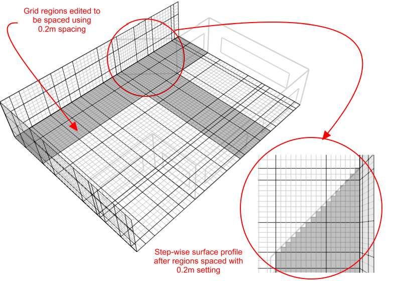

Due to the non-linearity, the equation set cannot be solved using analytical
techniques, which necessitates the requirement for a numerical method. The
numerical method employed by DesignBuilder involves re-casting the differential
equations into the form of a set of finite difference equations by sub-dividing the
required building space (or calculation domain) into a set of non-overlapping
adjoining rectilinear volumes or cells, which is collectively known as a finite volume
grid. The equation set is then expressed in the form of a set of linear algebraic
equations for each cell within the grid and the overall set of equations is solved using
an iterative scheme. The non-linearity of the equation set is accounted for by the use
of a nested iterative scheme whereby each dependent variable equation set (velocity
components, temperature, etc.) are themselves solved iteratively within an overall
outer iterative loop and at the termination of each outer iteration, the most recent
values of the dependent variables are fed back into the dependent variable
coefficients. The outer iterative loop is repeated until the finite difference equations
for all cells are satisfied by the current values of the appropriate dependent variables,
at which point the scheme is said to have ‘converged’. An appreciation of the
requirement for convergence and the nested iterative procedure used to achieve it will
help in understanding the meaning of the various calculation options that are
described in the ‘Conducting CFD Calculations’ section.

The Iterative Nature of the Procedure

The calculation procedure has been developed to ensure that the iterative solution of
the equation set would be guaranteed to converge if the equation coefficients were
constant. However, the equation set is non-linear and the coefficients actually contain
the dependent variables themselves, and consequently convergence cannot be
guaranteed in all cases. Although in the majority of cases, as long as the dependent
variables and particularly the velocities only change slowly, a converged solution is
normally achieved.

The main mechanism to ensure that the variables change slowly is that of false time
steps. The finite difference equation set is formulated in the form of a transient
equation set although the calculations are steady state, i.e. essentially a ‘snap-shot’ in
time. The reason for this formulation is that the transient term behaves as a very
effective relaxation method, which can slow the change in dependent variables in
order to arrive at a more stable solution. The false time step is the time step used in
the pseudo-transient term of the dependent variable equation.

Creating Model Geometry for CFD

If you have already created a model for the purpose of an additional analysis (e.g.
thermal simulation or SBEM calculation), you can use exactly the same model for
CFD, although you should read the next section on the finite volume grid and
geometric considerations. On the other hand, if you intend to conduct a CFD analysis
from scratch, you should refer to the ‘Building Models’ section of the DesignBuilder
Help for information on creating models.

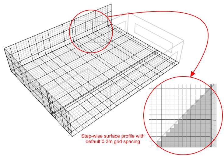
The Finite Volume Grid and Geometric Modelling Considerations

The calculation method requires that the geometric space across which the
calculations are to be conducted is first divided into a number of non-overlapping
adjoining cells which are collectively known as the finite volume grid.

When a CFD project is created, a grid is automatically generated for the required
model domain by identifying all contained model object vertices and then generating
key coordinates from these vertices along the major grid axes. These key coordinates,
extended from the X, Y and Z-axes across the width, depth and height of the domain
respectively are known as ‘grid lines’. The distance between grid lines along each axis
is known as a grid ‘region’ and these regions are initially spaced employing user-
defined default grid spacing in order to complete the grid generation. The grid used by
DesignBuilder CFD is a non-uniform rectilinear Cartesian grid, which means that the
grid lines are parallel with the major axes and the spacing between the grid lines
enables non-uniformity.

For example, looking at a simple building block with a single component assembly
representing a table:

The resulting grid, generated with 0.3m default grid spacing would be as follows:

By default, grid regions are spaced uniformly using a spacing that is calculated to be
as close to the user-defined default grid spacing as possible. Notice the narrow regions
created between key coordinates associated with the tabletop and table legs. In this
case, the distance between these key coordinates is of an acceptable value. However,
very narrow regions resulting in long narrow grid cells or cells having a high aspect
ratio should be avoided, as they tend to result in unstable solutions that can fail to
converge. Highly detailed component assemblies can result in very large numbers of
closely spaced key coordinates resulting in cells having high aspect ratios. Large
numbers of key coordinates can also lead to overly complex grids and
correspondingly high calculation run times and excessive memory usage which can be
avoided by replacing very detailed assemblies with cruder representations for the
purpose of the CFD calculation. However, where very narrow grid regions are
unavoidable, adjacent grid lines formed from key coordinates can be merged together
using the merge tolerance setting which is accessed through the new CFD analysis
dialogues (see the ‘Setting Up a New External CFD Analysis’ and ‘Setting Up a New
Internal CFD Analysis’ sections). For instance, in the above example, if the table
assembly had been located closer to the edge of the adjacent window, this could result
in unacceptably close grid lines:

These closely spaced grid lines can be merged by creating a new analysis and
increasing the grid line merge tolerance setting to say 0.025m:

Due to the strict rectilinear nature of the grid, grid cells that lie in regions outside of
the domain required for calculation are ‘blocked-off’ in order to cater for irregular
geometries. It is important to take this into account when creating a model in order to
maximise the efficiency of grid generation and/or to ensure that surface CFD
boundaries will lie in the plane of a major grid axis to achieve accuracy of boundary
representation. In some cases, the model may be rotated in order to ensure that most
of the wall surfaces are orthogonal with respect to the grid axes. To take an extreme
example, if a simple rectangular space has been drawn at a 45° angle to the Z-axis:

The resulting grid, generated using 0.3m default grid spacing, contains a great deal of
redundancy in the form of blocked-off regions and inaccuracy of surface
representation:

If the block is first rotated, to be aligned with the X-axis:

The resulting grid exhibits no redundancy and there is no inaccuracy in surface
representation:

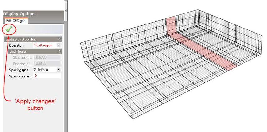
The accuracy of the representation of non-orthogonal surfaces can be improved by
using smaller default grid spacing and in some cases specific grid regions can be
modified to increase accuracy in a more localised fashion as illustrated by the
following example:

Grid generated using default 0.3m grid spacing:

Using the ‘Edit CFD Grid’ tool, the grid spacing within just the regions spanning the
angled section is reduced to 0.2m to improve the representation:

Grid regions between key coordinates can also be spaced using non-uniform spacing
options and additional key coordinate regions can be added. Further information is
provided on grid modification in the ‘Editing the CFD Grid’ section.

Building Levels and CFD Analyses

Internal CFD analyses can be conducted at zone, building block and building levels.
Calculations can also be conducted for single zones that span several blocks by
connecting them with holes and using the ‘merge zones connected by holes’ model
option setting. External analyses can only be conducted at the site level.

CFD Boundary Conditions

An important initial concept for CFD analyses is that of boundary conditions. Each of
the dependent variable equations requires meaningful values at the boundary of the
calculation domain in order for the calculations to generate meaningful values
throughout the domain. These values are known as boundary conditions and can be
specified in a number of ways. The specification of boundary conditions for external
analyses is relatively straightforward and just requires setting the building exposure,
wind velocity and wind direction and this is done using a single dialogue box.
However, internal analysis boundary conditions tend to be a bit more involved and

can require the addition of zone surface boundaries such as supply diffusers, extract
grilles, temperature and heat flux patches and also the incorporation of model
assemblies representing occupants, radiators, fan-coil units, etc. DesignBuilder
provides default wall and window boundary temperatures automatically but it is
important that you check that these defaults are appropriate ones and that you
correctly specify any additional boundary conditions required for your project.

Boundary Conditions for Internal CFD Analyses

Internal boundary conditions can be defined in three ways:

   1. Default wall and window temperatures can be defined for all zone surfaces.
   2. Zone surface boundary conditions including supply diffusers, extract grilles,
      temperatures and heat fluxes can be added in the form of surface patches using
      a similar method to that used for adding windows and doors.
   3. Component blocks and component assemblies can be defined as temperature
      or heat flux boundaries.

Default Wall and Window Temperatures

All zone surfaces within a model have default wall and window boundary
temperatures. These boundary temperatures are inherited from the building level
down to the zone surface level and may be set at any intermediate level. This
mechanism provides a convenient method for defining wall and window temperature
boundary conditions throughout a building model in the absence of imported
EnergyPlus boundary data (see ‘Importing EnergyPlus Output Data’).

Default wall and window boundary temperatures can be accessed under the ‘CFD
Boundary’ header on the ‘Construction’ tab:

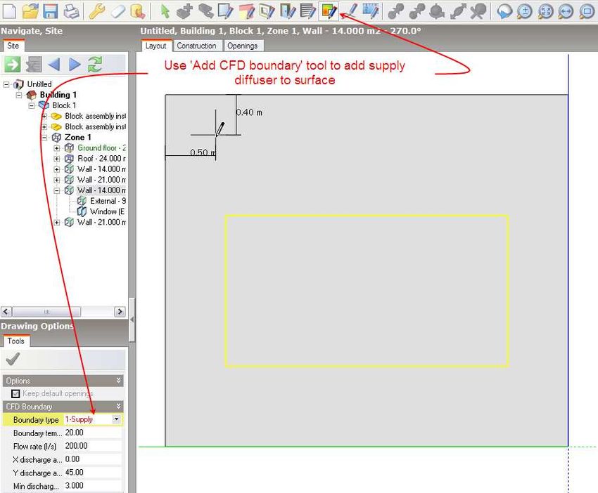
Zone Surface Boundaries

Supply diffusers, extract grilles, temperature and heat flux patches can be added to
zone surfaces using the ‘Add CFD boundary’ tool.

To add a surface boundary, move down to the surface on which you want to locate the
boundary, either by selecting it from the model navigator or by navigating to it in the
Edit screen. At the surface level, you can then select the ‘Add CFD boundary’ tool
from the toolbar:

You can draw a CFD boundary on to the surface in exactly the same way that you
would draw a window. Please refer to the ‘Add window’ Help section for details of
drawing windows.

After selecting the ‘Add CFD boundary’ tool, the boundary settings are displayed on
the ‘Drawing Options’ data panel. You can select the required boundary type from the
‘Boundary type’ drop list. The following boundary types are available for surfaces of
all orientations:

1 – Supply (general purpose HVAC supply diffuser)
4 – Extract (HVAC extract grille)
5 – Temperature (surface temperature patch)
6 – Flux (surface heat flux patch)

The following additional boundary types for multi-directional diffusers will appear for
ceiling surfaces only:

2 – Four-way (four-way supply diffuser)
3 – Two-way (two-way supply diffuser)

Various settings are available depending on the boundary type:

1 - Supply:

     Boundary temperature (°C):

     Enter the required temperature of the air entering the space.

     Flow rate (l/s):

     Enter the supply volume flow rate.

     X-discharge angle (°):

     This setting allows you to define the discharge angle between the local surface
     X-axis and an inward facing normal to the surface. At the surface level, taking a
     normal view from the inside of the zone to the surface, the X-axis discharge
     angle is positive between the normal and the positive X-axis (i.e. the axis
     pointing towards the right) and negative between the normal and the negative X-
     axis (i.e. the axis pointing towards the left). For example to define a discharge
     angle of 45° pointing towards the left of the centre of a diffuser, looking at it
     from the inside of the zone, you would enter –45. On the other hand, to define a
     discharge angle of 45° pointing towards the right of the centre, you would enter
     45:

Y-discharge angle (°):

    This setting allows you to define the discharge angle between the local surface
    Y-axis and an inward facing normal to the surface. At the surface level, taking a
    normal view from the inside of the zone to the surface, the Y-axis discharge
    angle is positive between the normal and the positive Y-axis (i.e. the axis
    pointing upwards) and negative between the normal and the negative Y-axis (i.e.
    the axis pointing downwards). For example to define a discharge angle of 45°
    pointing downwards from the centre of a diffuser, looking at it from the inside
    of the zone, you would enter –45. On the other hand, to define a discharge angle
    of 45°, pointing upwards from the centre, you would enter 45:

    Minimum discharge velocity (m/s):

    The minimum discharge velocity is the minimum required velocity at the face of
    the diffuser. Supply diffusers are created using a number of elements, the areas
    of which are determined by combining the specified volume flow rate together
    with the minimum discharge velocity. The maximum linear dimension of each
    component element is currently 'hard-set' at 0.2m.

2 – Four-way

    Boundary temperature (°C):

Enter the required temperature of the air entering the space.

    Flow rate (l/s):

    Enter the supply flow rate.

    Multi-way diffuser discharge angle (°):

    Enter the discharge angle, which is the angle between the downward pointing
    normal and the diffuser jet:

    Minimum discharge velocity (m/s):

    The minimum discharge velocity is the minimum required velocity at the face of
    the diffuser. Four-way diffusers are created using four separate elements, one
    located at each edge of the diffuser, the area of each being determined by
    combining the specified volume flow rate together with the minimum discharge
    velocity.

3 – Two-way

    Boundary temperature (°C):

    Enter the required temperature of the air entering the space.

    Flow rate (l/s):

Enter the supply flow rate.

     Multi-way diffuser discharge angle (°):

     Enter the discharge angle, which is the angle between the downward pointing
     normal and the diffuser jet (see illustration in ‘Four-way’ section).

     2-way diffuser discharge direction:

     Enter the local surface axis along which the diffuser is to discharge:

     Minimum discharge velocity (m/s):

     The minimum discharge velocity is the minimum required velocity at the face of
     the diffuser. Two-way diffusers are created using two separate elements, one on
     either side of the diffuser along the discharge axis, the area of each being
     determined by combining the specified volume flow rate together with the
     minimum discharge velocity.

2 – Extract

     Flow rate (l/s):

     Enter the extract flow rate.

3 – Temperature

     Boundary temperature (°C):

     Enter the required temperature for the patch.

4 – Flux

     Heat flux (Wm-2):

     Enter the required heat flux for the patch.

Using Component Blocks and Component Assemblies as CFD Boundaries

Component blocks and assemblies can be used for CFD analyses to simply allow for
the effect of obstructions on the airflow. However, they also allow the definition of
CFD boundary attributes to enable them to act as constant temperature surfaces or
heat flux sources and can also be modified to behave as non-solids to allow air to pass
through them.

Component Blocks

CFD attributes for component blocks are inherited down from the building level to
component blocks located at both building and building block levels. CFD attributes
for component blocks are accessed under the ‘Component block’ header on the
‘Construction’ tab:

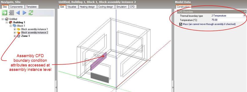
Assemblies

The CFD assembly library that is provided with DesignBuilder contains a number of
pre-defined assemblies that can be used to add items such as occupants, radiators and

furniture. Some of these pre-defined assemblies already have CFD boundary
attributes associated with them, e.g. occupant assemblies have a defined heat flux of
90W. You can also define your own assemblies for use in CFD analyses and you will
find details of how to do this in the ‘Assemblies’ Help section.

CFD attributes for component assemblies are inherited from the parent assembly to
instances of the assembly at the building and building block levels. CFD attributes for
assemblies are accessed from the ‘Construction’ tab after moving down to an
assembly instance level by clicking on it in the navigator or double-clicking on it in
the Edit screen. It is important to understand that if you change an attribute for a
specific instance of an assembly, the attributes will be changed for all other instances
of the same assembly.

The following CFD boundary settings are available for both component blocks and
component assemblies:

Thermal boundary type:

The thermal boundary type can be set to one of the following:

1 – None:

Component block does not act as a CFD boundary condition.

2 – Temperature:

Component block acts as a fixed temperature CFD boundary condition.

3 – Flux:

Component block supplies a fixed heat flux to the surroundings.

Temperature (°C):

If the thermal boundary type has been set to ‘Temperature’, enter the temperature of
the block.

Flux (W):

If the thermal boundary type has been set to ‘Flux’, enter the heat emission of the
block.

Mass:

This setting determines whether or not the block will act as a physical obstruction to
the surrounding flow. In some cases, it may be desirable to fix the temperature or flux
of the component but allow air to pass through the block, e.g. to represent an
occupancy flux throughout a large volume without needing to locate individual
occupants.

Setting Up a New External CFD Analysis

To create a new external CFD analysis, first make sure that you have selected the Site
object in the model navigator and then click on the CFD tab:

The ‘New CFD Analysis Data’ dialogue is displayed which allows you to name the
analysis, define grid generation variables, wind data and the extents of the domain to
be included in the analysis:

Default Grid Spacing

On entry to the CFD screen after completing and closing the new CFD analysis
dialogue, the CFD grid is automatically generated throughout the overall external
domain extents. The grid is created by first determining key points obtained from
constituent model blocks along the major axes, the distance between each of these key
points being known as regions. Each CFD grid region along each major axis is
automatically spaced using the ‘default grid spacing’ dimension.

Grid Line Merge Tolerance

A potential problem when generating the grid is the creation of cells with a high
aspect ratio that can lead to instability in the equation solver. In order to avoid such
cells, grid lines that are very close together can be merged. The ‘grid line merge
tolerance’ is the maximum dimension that will be used in determining whether or not
to automatically merge grid lines.

Wind Velocity

Enter the required free stream wind velocity in m/s (measured at 10m above ground).

Wind Direction

The wind direction is defined clockwise from North. The default direction is 270°, i.e.
Westerly.

Wind Exposure
The free stream wind velocity is corrected for height above ground and surrounding
terrain using an empirical relationship recommended by ASHRAE:

d am h a
                                 v =v    
                                   *     m
                                     1h        d
                                        m  

                               Boundary layer height d (m)          Flow exponent a
Open country                            270.00                           0.14
Suburban                                370.00                           0.22
Urban                                   460.00                           0.33

Site Domain Factors
The length, width and height site domain factors are multipliers that are applied to the
overall dimensions of the building model in order to arrive at an external volume or
domain across which the analysis is carried out. The default factors are 3.0 applied to
the length and width and a factor of 2.0 that is applied to the model height.

After clicking on the OK button, the CFD screen is displayed showing the model in
conjunction with the site domain object:

Setting Up a New Internal CFD Analysis

To create a new external CFD analysis, first make sure that you have selected the
appropriate level object (building, building block or zone) in the model navigator and
then click on the CFD tab:

The ‘New CFD Analysis Data’ dialogue is displayed which allows you to name the
analysis and define grid generation variables:

Default Grid Spacing

On entry to the CFD screen after completing and closing the new CFD analysis
dialogue, the CFD grid is automatically generated throughout the overall external
domain extents. The grid is created by first determining key points obtained from
constituent model blocks along the major axes, the distance between each of these key
points being known as regions. Each CFD grid region along each major axis is
automatically spaced using the ‘default grid spacing’ dimension.

Grid Line Merge Tolerance

A potential problem when generating the grid is the creation of cells with a high
aspect ratio that can lead to instability in the equation solver. In order to avoid such
cells, grid lines that are very close together can be merged. The ‘grid line merge

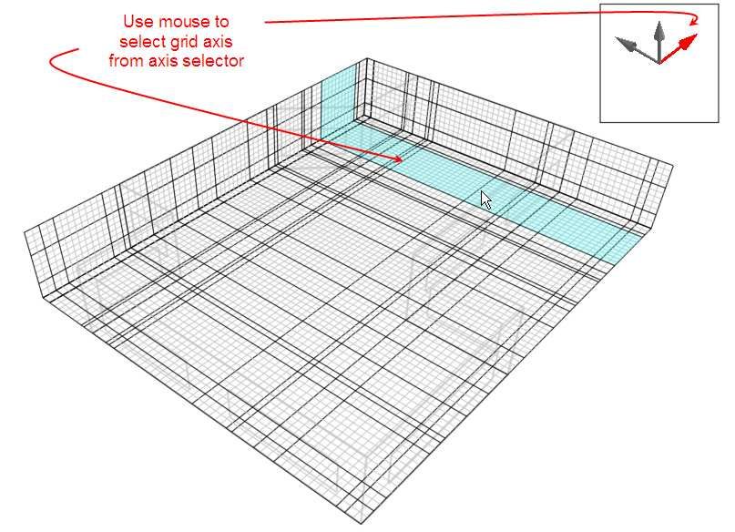
tolerance’ is the maximum dimension that will be used in determining whether or not
to automatically merge grid lines.

Editing the CFD Grid

As soon as a new analysis data set has been created, a default CFD grid is generated
using the default grid spacing defined as part of the data set. The default grid may be
edited using the ‘Edit CFD Grid’ tool which allows you to change the spacing used
for default regions, insert additional regions or remove previously inserted regions.

When you select the ‘Edit CFD Grid’ tool, the grid is displayed with the building
outline overlaid as a ghosted wire frame. Grid regions are displayed along the major
axes bounded by dark grey lines, the auto-generated grid region spacing lines being
displayed in a lighter grey. The currently selected grid region is selected in cyan or
yellow if the region is a non-default inserted region. To select regions on one of the
other major axes, you can change the axis by clicking on the required axis of the axis
selector displayed at the top right of the screen:

To edit a grid region, move the mouse cursor across the grid to the required region
that will highlight to indicate that it has been selected and then click the mouse button.

The selected region will then highlight in red and the ‘Edit CFD Grid’ data panel will
be displayed at the bottom left of the screen:

The following settings are available on the ‘Edit CFD Grid’ data panel:

Operation:

1 – Edit Region:

Change the spacing of the currently selected region.

2 – Insert Region

Insert a new custom key coordinate at a defined point in the current region to form an
additional region.

3 – Remove Region

This option is only available if the current region has been previously inserted and
allows you to remove it.

New coordinate (m):

If the ‘Insert Region’ operation has been selected, this setting is displayed allowing
you to define a custom coordinate within the current region. Note that the coordinate
must lie in the range defined by the displayed start and end coordinates.

Spacing Type:

The spacing type can be set to one of the following:

1 – None:

The region is not sub-divided.

2 – Uniform:

The region is sub-divided into a number of equal sub-divisions, the dimension of
which is calculated to be as close to the specified ‘Spacing dimension’ as possible.

3 – Increasing power-law:

The location of each sub-division grid line within the region increases as the power of
the spacing number, which starts at the beginning of the region. So that if i represents
the index number of the grid line counted from the start of the region, the coordinate
of the ith sub-division grid line is calculated using the following relationship:
xi=(region dimension)(i/n)power+xs

4 – Decreasing power-law:

The location of each sub-division grid line within the region decreases as the power of
the spacing number, which starts at the end of the region. So that if i represents the
index number of the grid line counted from the start of the region, the coordinate of
the ith sub-division grid line is calculated using the following relationship: xi=(region
dimension)[1-(i/n)power]+xs

5 – Symmetric power-law:

The coordinate of the ith sub-division grid line is calculated using both increasing and
decreasing power-law relationships that meet at the middle of the region:

For i = n/2: xi=[(region dimension)/2][2-(2i/n))power]+xs

Spacing dimension (m):

If the uniform spacing type has been selected, this setting is displayed and allows you
to enter the dimension used for sub-dividing the region.

Spacing power:

If the Increasing/Decreasing/Symmetric power law spacing type has been selected,
this setting is displayed and allows you to enter the power used in the associated
power-law spacing relationship.

Number of divisions:

If the Increasing/Decreasing/Symmetric power law spacing type has been selected,
this setting is displayed and allows you to enter the number of divisions used in the
associated power-law spacing relationship.

After selecting an operation and adjusting the required settings, you then need to click
on the ‘Apply changes’ button to update the selected grid region with the current
settings.

Setting Up CFD Cell Monitor Points

The CFD calculation process is iterative and is considered to have completed once
‘convergence’ has been achieved (see ‘CFD Calculations and Convergence’ section).
The main indicator for convergence is the point at which the finite difference
equations for all cells are satisfied by the current values of the appropriate dependent
variables. However, it can be very useful in many cases to monitor the variation of the
dependent variables at specific locations throughout the calculation domain in order to
observe the point at which they stabilise. It may be acceptable, in many cases, to
terminate a calculation as soon as the dependent variables have achieved adequate
stability but before the residuals have arrived at their defined termination values.
When a project is first created, a default central cell monitor point is automatically
added to the domain. The ‘Define CFD monitor points’ tool enables you to identify up
to ten cells throughout the calculation domain at which you want to monitor the
variation of the calculated variables. After selecting the ‘Define CFD monitor points’
tool, the cell monitor screen is displayed which includes the model view together with
a cell selection frame, perpendicular to the currently selected axis. You can select a
plane along the current axis by moving the mouse cursor across the model in the
direction of the axis. To change the axis, click on the required axis on the axis selector
tool, which is located at the top right of the screen:

After selecting the required axis, move the cell selection frame along the axis, and
then click the mouse button to select a plane at the required distance along the axis. A
cell selection grid is then displayed in the selected plane allowing you to move the
mouse cursor to the required cell in that plane:

After moving the mouse cursor to the required cell, click the mouse button to display
the cell monitor data panel at the bottom left of the screen.

The following settings are available on the cell monitor data panel:

Operation:

This control is only active if you have selected a cell for which a monitor point has
already been defined. The following options are available:

1 – Update cell

Add a monitor point or edit the name of a previously defined point.

2 – Remove cell

Remove a previously defined monitor point.

Monitor location name:

Enter name for monitor point.

After changing the required settings, click on the ‘Apply changes’ button to update
the selected cell. You can quit out of the ‘Define CFD monitor points’ tool by
pressing the ESC key or selecting another tool.

CFD Grid Information

Information about the CFD grid can be obtained using the ‘Show CFD grid statistics’
tool, which displays the CFD grid statistics dialogue:

If the maximum cell aspect ratio exceeds the allowable limit of 50 or the required
memory exceeds the physical memory available, the ‘Check’ will indicate a failure:

Conducting CFD Calculations

Please refer to the ‘CFD Calculations and Convergence’ section for an overview of
the calculation methodology that will help in understanding the concepts used to
initialise, control and monitor the calculations.

To conduct the calculations, click on the ‘Update calculated data’ tool. If a problem is
found with the grid generation, the CFD Grid Statistics dialogue is displayed showing
the error. There are three possible error conditions:

Maximum cell aspect ratio exceeds the limit - you will need to delete the existing
project and create a new one either reducing the default grid spacing dimension or
increasing the grid line merge tolerance by a suitable amount (see the ‘CFD Results
Manager’ section).

Required memory exceeds the available memory - you will need to delete the existing
project and create a new project with larger default grid spacing or consider
simplifying the problem definition in terms of complexity of assemblies, etc.

Flow imbalance – The total flow rate specified for supply diffusers does not balance
with the total flow rate specified for extract grilles. You will need to add supply
diffusers or extract grilles or edit the existing flow rates to establish the correct
balance

 If no problem is encountered in creating the grid, the ‘Edit Calculation Options’
dialogue will be displayed:

The ‘Edit Calculation Options’ dialogue is divided into two main sections, the
Residuals and Cell Monitor graphs and the Calculation Options Data panel. There are
also a group of buttons at the bottom of the dialogue, which allow you to control the
calculations:

Start

Start, or if the calculations have been paused, re-start the calculations.

Pause

Interrupt or pause the calculations. Once the calculations have been paused, the
calculation dialogue can be temporarily closed in order to review the results.

Reset

After pausing the calculations, the calculations may then be re-initialised to start from
scratch. If the solution is found to diverge and you pause the calculations to decrease
the velocity false time steps, you will then need to reset the calculations before re-
starting.

Calculation Options Data

The calculation settings panel incorporates the following settings:

Turbulence Model:

The following turbulence models are available:

1 – k-ε

This model is one of the most widely used and tested of all turbulence models,
belonging to the so-called RANS (Reynolds Averaged Navier-Stokes) family of
models. These models involve replacing the instantaneous velocity in the Navier-
Stokes and energy equations with a mean and fluctuating component. The resulting
equations give rise to additional terms known as Reynolds stresses and turbulent heat
flux components. Reynolds stresses are replaced with terms involving instantaneous
velocities where molecular viscosities are substituted for effective viscosities and a
similar substitution is conducted for the energy equation. The effective viscosity is the
sum of the molecular viscosity and a turbulent viscosity, which is derived from the
turbulence kinetic energy and the dissipation rate of turbulence kinetic energy:

            k2
µt = Cµ ρ
            ε

where k= turbulence kinetic energy and ε = dissipation rate of turbulence kinetic
energy

k and ε are both derived from partial differential equations which are in turn derived
from a manipulation of the Navier-Stokes equations.

2 – Constant effective viscosity

The constant effective viscosity model is a much simpler approach and involves the
replacement of the molecular viscosity in the Navier-Stokes equations with a constant
effective viscosity (typically in the order of 100-1000). Although this model is
incapable of modelling local turbulence or the transport of turbulence, it is
computationally much less expensive than the k-ε model and can be numerically
much more stable.

Discretisation scheme

The calculation process involves replacing the defining set of partial differential
equations with a set of finite difference equations. The conventional approach to this
is to use a Taylor’s series formulation, which leads to a set of central difference
equations. However, although this approach is physically realistic for diffusion, it is
not found to be realistic for convection because of the one-way nature of convection,
i.e. upwind conditions affect downwind conditions but not the reverse.

The following discretisation schemes are available:

1 - Upwind

The upwind scheme allows the convective term to be calculated assuming that the
value of the dependent variable at a cell interface is equal to the value at the cell on
the upwind side of the interface.

2 – Hybrid

The hybrid scheme combines a strict central difference treatment (-2

Isothermal:

Temperature is assumed to be constant throughout the calculation domain and the
energy equation is removed from the calculations.

Surface heat transfer:

The following surface heat transfer options are available:

1 – Calculated

Surface heat transfer coefficients are calculated using wall functions if the k-ε
turbulence model has been selected.

2 – User-defined

Surface heat transfer coefficients can be define for ceilings, wall and floors.

Initial conditions:

In some cases, a faster solution can be achieved by setting the initial conditions closer
to the final expected conditions.

Cell monitor:

Select any defined cell monitor point and associated dependent variable to be
displayed on the cell monitor (see ‘Setting Up CFD Cell Monitor Points’ section).

Residual Display

Select the dependent variables and/or mass for which residuals are to be displayed in
the residuals monitor. The mass residual is similar to the dependent variable residuals
but is extracted from a continuity equation mass balance for each cell.

Dependent Variable Control Settings:

The calculations involve a nested iterative scheme whereby dependent variable
equations are solved iteratively within an overall outer iterative loop (see ‘CFD
Calculations and Convergence’ section). The dependent variable control settings
enable control inner iterative dependent variable calculations.

     Inner Iterations:

     The number of iterations used for the calculation of the dependent variable.

     False Time Step:

     The finite difference equation set is formulated in the form of a transient
     equation set although the calculations are essentially a ‘snap-shot’ in time. The
     reason for this formulation is that the transient term behaves as a very effective

relaxation method, which can slow the change in dependent variables in order to
     arrive at a more stable solution. The false time step is the time step used in the
     pseudo-transient term of the dependent variable equation. For forced convection
     flows, a ‘best-guess’ optimal false time step is automatically calculated for
     velocities, however for buoyancy driven flows, a default value of 0.2 is used.
     Reducing the false time step has the effect of slowing down the change in the
     dependent variable and can be a helpful remedy for unstable solutions.

     Relaxation Factor:

     This is the ‘text book’ relaxation method, which can be used to allow only a
     proportion of the calculated value of the current iteration dependent variable to
     be assigned to the variable. However, the false time step is normally the
     preferred method of achieving under-relaxation.

     Termination Residual

     The outer iterative calculation loop is repeated until the finite difference
     equations for all cells are satisfied by the current values of the appropriate
     dependent variables, at which point the scheme is said to have ‘converged’. The
     dependent variable residual is the maximum residual quantity for the equation
     balance across all cells in the domain. The solution is deemed to have converged
     for each dependent variable when the residual is less than the termination
     residual.

Residuals and Cell Monitor Graphs

The value of each dependent variable residual together with the mass residual is
plotted on the residuals graph, at the end of each outer iteration of the calculation.
You can use the residuals plot to monitor the overall convergence of the solution and
to determine whether or not any remedial action is required.

When considering the residual plots, you should bear in mind that the residuals can
fluctuate quite markedly throughout the period of the calculations and in some cases
rise appreciably before falling and so you need to get an idea of the overall trend after
several hundred iterations. The following screenshot shows a plot of residuals and a
default centrally located monitor cell plot for the internal analysis illustrated in the
next ‘Displaying Results’ section. Notice that the monitored velocity has reached a
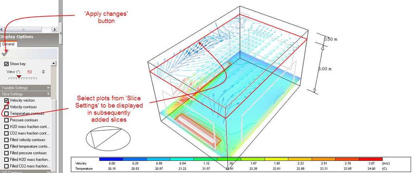
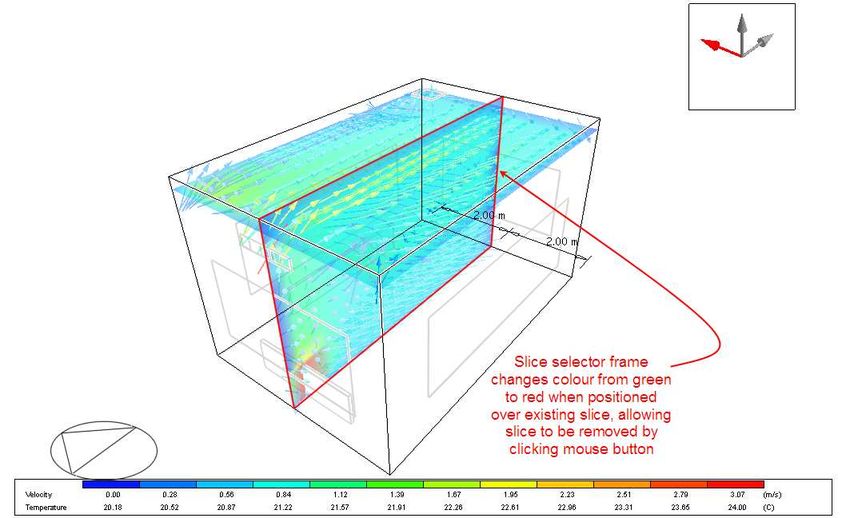
steady final value.

If you notice that the residuals are fluctuating wildly or steadily increasing over
several hundred iterations, you should pause the calculations and take remedial action
(see ‘Convergence Difficulties and Troubleshooting’ section).

The cell monitor graph displays the variation in the selected dependent variable for
the currently selected monitor cell (see ‘Setting Up CFD Cell Monitor Points’ section
and ‘Cell Monitor’ setting in the ‘Calculation Options Data’ section above). The
variation of monitored cell point variables provides a good indication of solution
convergence, i.e. when the variation of the variable stabilises.

Convergence Difficulties and Troubleshooting

If the plotted residuals are found to diverge or fluctuate significantly, in many cases
you will find that the situation can be improved by reducing the false time steps for
the velocity components. The recommended procedure is to continuously half the
time steps until a more stable solution is found.

Displaying Results

After completing or pausing the calculations, the CFD ‘Display Options’ data panel
and the ‘Select CFD slice’ tool become active.

The main mechanism for displaying results is the slice tool that allows you to select a
slice, along one of the main grid axes and perpendicular to it, within which can be
displayed any of the selected results display plots. After selecting the ‘Select CFD
slice’ tool, the CFD results screen is displayed which includes the model view
together with a slice selection frame, perpendicular to the currently selected axis. You

can select a slice along the current axis by moving the mouse cursor across the model
in the direction of the axis. To change the axis, click on the required axis on the axis
selector tool, which is located at the top right of the screen:

After selecting the required axis and moving the slice selector frame to the required
position along the axis, click the mouse button to add the slice to the display. Notice
that as you move the slice selection frame to a slice that was previously added to the
display, the frame colour changes from green to red and if you click the mouse button,
the slice is removed from the display:

Slice variable plots are selected under the ‘Slice Settings’ header on the ‘Display
Options’ data panel and controlled under the ‘Variable Settings’ header:

Note that any modifications made to items on the ‘Display Options’ data panel will
only come into effect after clicking on the ‘Apply changes’ button.

The ‘Variable Settings’ group contains groups of variable banding data for velocity,
temperature and pressure variables. Also, under the variable settings ‘Velocity’
header, there are two velocity vector settings, ‘Maximum vector length’ and ‘Velocity
scale factor’. Velocity vectors are displayed as arrows, the length of which
corresponds to the magnitude of the velocity and with the default vector scale factor
of 1.0, a length of 1.0m corresponds to a magnitude of 1.0m/s. The maximum vector
length is the maximum length of a vector that will be displayed to prevent the display
from becoming cluttered with excessively large vectors. Any vector, which has a
magnitude greater than this maximum, will be displayed translucently to distinguish it
from vectors with lengths that do represent magnitude.

The variable banding data comprises the defined band range, followed by twelve
contour band values within the defined range. The band range defines the minimum
and maximum variable values between which data will be displayed and the band
values are the actual values within that range that are displayed in the form of
contours or in the case of velocity vectors, vector colours. The default minimum and
maximum variable display values are extracted from the calculated values and this
range is then divided into twelve equal increments in order to arrive at the dependent
variable contour bands. Each contour band can be edited or switched off altogether.
When the band range values are modified, the individual band values are
automatically re-calculated.

The ‘Slice Settings’ group is used to select the plots required to be included in
subsequently added slices.

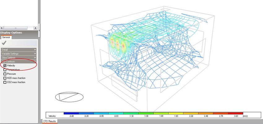
The last item on the ‘Display Options’ data panel is the 3-D contours group that
allows you to select any of the available variables for which a 3-D contour plot is
required:

The ‘Display Options’ data panel also includes a ‘Detail’ group that allows you to
modify general model render settings (see ‘Visualisation’ section), together with
specific CFD model display options:

CFD view type:

The following view types are available:

1 – Rendered

This is the conventional visualisation rendered view (see ‘Visualisation’ section).

2 – Wire-frame

The wire frame displays the model fabric in wire frame and all component blocks,
assemblies, partitions and slabs are displayed as 3D objects with hidden-line removal.
This option can be used to provide a clearer view of the results.

Antialiasing

See ‘Visualisation’ section.

Show shadows

This setting is only available if the ‘Rendered’ CFD view type has been selected. See
‘Visualisation’ section for details on shadow rendering.

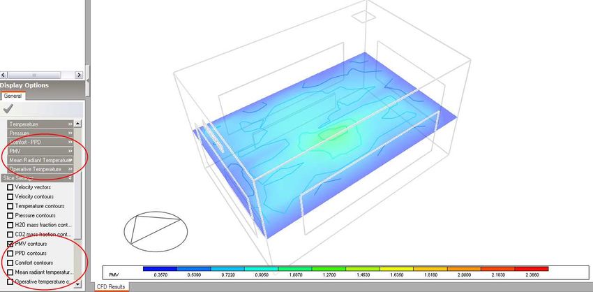
Display partitions

This setting is only available if the ‘Wire-frame’ CFD view type has been selected.
The ‘Display partitions’ setting allows you to switch off the display of internal
partitions to obtain an unobstructed view of results.

Display floors and roofs

This setting is only available if the ‘Wire-frame’ CFD view type has been selected.
The ‘Display floors and roofs’ setting allows you to switch off the display of floor and
roof slabs to obtain an unobstructed view of results.

Show North arrow

See ‘Visualisation’ section

Show key

Toggles the display of the variable contour key

View

See ‘Visualisation’ section

Conducting CFD Comfort Calculations

After completing or pausing the CFD calculations (see ‘Conducting CFD
Calculations’ section), the ‘Update CFD comfort’ tool will become enabled. After
selecting the ‘Update CFD comfort’ tool, a progress bar will be displayed indicating
that mean radiant temperature (MRT) calculations are in progress, followed by
another progress bar for the comfort calculations themselves. Either of these processes
can be cancelled at any time by clicking on the ‘Cancel’ button.

Comfort calculation metabolic rates and clothing levels are obtained from the data
entered under the ‘Metabolic’ header on the ‘Activity’ tab of the model data panel.

After completing the calculations, various additional comfort display variables are
available on the ‘Display Options’ data panel:

PMV
PPD
Comfort Indices
Mean Radiant Temperature
Operative Temperature

CFD Results Manager

The ‘CFD results manager’ tool allows you to create new CFD projects, open existing
projects or remove existing projects. For example, considering the internal analysis
example illustrated in the ‘Displaying Results’ section, you may want to conduct
another analysis after moving the position of a radiator in order to look at the effect on
air distribution. You would first go to the Edit screen and modify the radiator layout:

After returning to the CFD screen, you can then click on the ‘CFD results manager’
tool to open the ‘CFD Results Manager’ dialogue:

The CFD Results Manger dialogue incorporates a list of all available projects together
with buttons that allow you to create a new project, open a project or delete a project.
For each project entry in the list, the first column indicates the project name, the
second column the model domain object used for the calculations (site, building,
building block, zone) and the third column indicates whether or not the model
geometry contained within the results is up-to-date. In this case, you would click on
the ‘New’ button to create a new project:

See the ‘Setting Up a New Internal CFD Analysis’ section for details of creating a
new internal analysis.

After creating the new analysis, you can then conduct the calculations:

You can then use the CFD Results Manager to open the previous project in order to
compare results: