Assessment North Sea Joint Monitoring Programme for Ambient Noise North Sea 2018 2020
←
→
Page content transcription
If your browser does not render page correctly, please read the page content below
Joint Monitoring Programme for Ambient Noise North Sea
                                2018 – 2020

                 Assessment North Sea
                                   WP 1
                            Deliverable/Task:

Authors:     Niels Kinneging and Jakob Tougaard
Affiliations: Rijkswaterstaat

Date: February 2021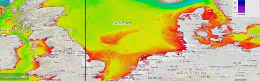
INTERREG North Sea Region
Jomopans

    2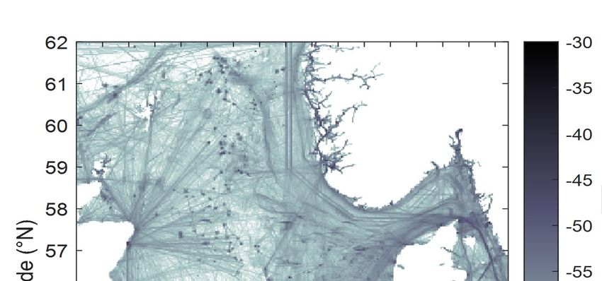
INTERREG North Sea Region
                                                                                           Jomopans

 Project Full Title              Joint Monitoring Programme for Ambient Noise North Sea
 Project Acronym                 Jomopans
 Programme                       Interreg North Region Programme
 Programme Priority              Priority 3 Sustainable North Sea Region

Colophon

Authors                                   Niels Kinneging (Project Manager)

Organization Name                         Rijkswaterstaat

Email                                     niels.kinneging@rws.nl

Phone                                     +31 6 5321 5242

 Version              Date        Review                    Initial   Approval              Initial
 Initial              5-2-2021

This report should be cited:
Kinneging, N.A. and Tougaard, J. (2021) Assessment North Sea. Report of the EU INTERREG Joint
Monitoring Programme for Ambient Noise North Sea (Jomopans), February 2021

                                                                                               3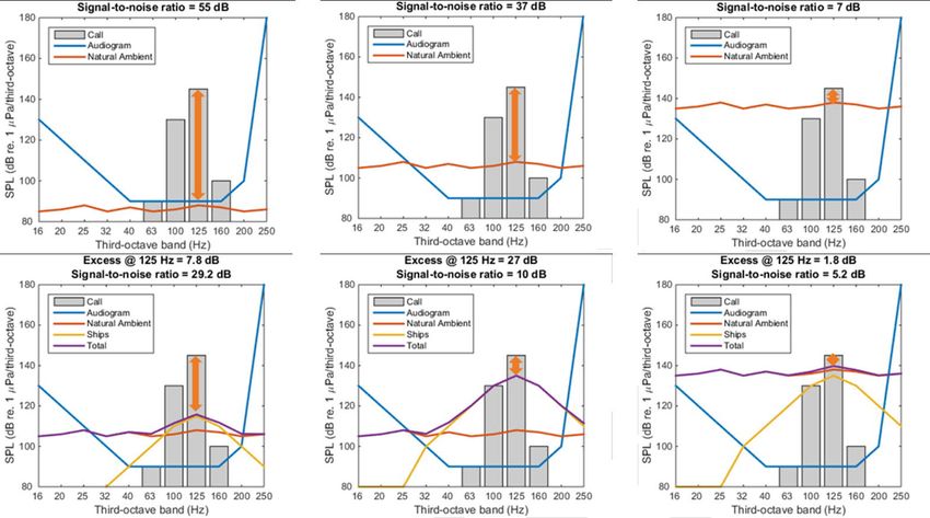
INTERREG North Sea Region
Jomopans

Table of contents
Summary 6
1               Introduction...................................................................................................................... 8
1.1             Thresholds for GES.......................................................................................................... 8
1.2             Introduction to effects of continuous noise (masking)......................................................... 8
1.3             Stepwise approach to monitoring and assessment .......................................................... 10
2               Stepwise assessment .................................................................................................... 12
2.1        Step 1-3. Collect information on human activities, source properties and environmental
properties 12
2.1.1           AIS and VMS ................................................................................................................. 12
2.1.2           Bathymetry .................................................................................................................... 13
2.1.3           Sea bottom composition ................................................................................................. 13
2.1.4           Others ........................................................................................................................... 14
2.2             Step 4. Modelling soundscape maps............................................................................... 14
2.3             Step 5. Measure long term acoustical parameters at several stations............................... 16
2.4             Step 6. Confidence maps ............................................................................................... 17
2.5             Assessment of continuous noise..................................................................................... 18
2.5.1           Assessment selected areas ............................................................................................ 19
3               Discussion ..................................................................................................................... 21
References ..................................................................................................................................... 22
Annex A         Dominance .................................................................................................................... 23

       4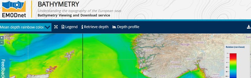
INTERREG North Sea Region
                Jomopans

                   5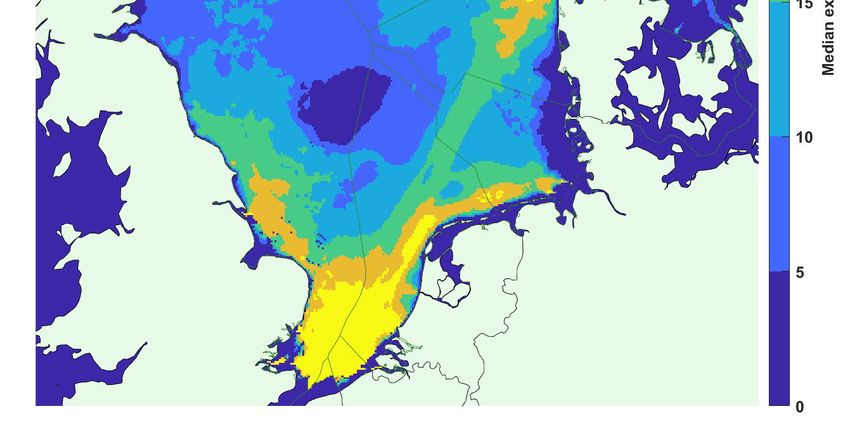
INTERREG North Sea Region
Jomopans

Summary

[to be written]

     6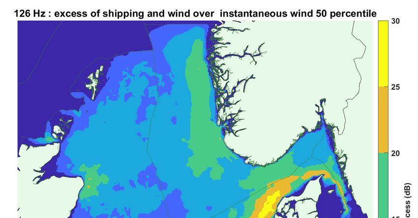
INTERREG North Sea Region
                Jomopans

                   7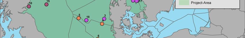
INTERREG North Sea Region
Jomopans

1     Introduction
1.1       Thresholds for GES
The concept of a threshold for Good Environmental Status is simple in principle, yet challenging when
it comes to actual implementation. The threshold should ideally be a single number, which can be used
to evaluate a one-dimensional index, G, derived from an assessment of the underwater noise in the
area under assessment. If the index GMRU is below the threshold GGES, the area is in GES; if not, the
area is not in GES.
The challenge is to get from the multi-dimensional real world, where noise is 4-dimensional (x,y,z and
t), with a number of co-variates and derived properties, such as frequency spectrum and dominant
source type. An enormous amount of information and detail is lost in the transformation from the actual
sound field (in the real world or modelled) in a geographical area into the one-dimensional index. What
is essential to observe is that the index preserves sufficient information to be informative about the
environmental conditions. In other words, the index must correlate with something of relevance to the
animals in the assessment area.

For continuous noise, there are two principal mechanisms by which the noise can affect animals:
masking of other sounds and behavioural disturbance. They are fundamentally different and should be
addressed differently. Masking means that an animal faces increased difficulties in detecting and
decoding other sounds (from conspecifics, prey, predators etc.) and ultimately means that the listener
fails to react to a signal it would otherwise have reacted to. Behavioural disturbance means that the
noise causes the receiving animal to change its behaviour into something else (fleeing, attention,
distraction etc.). The JOMOPANS pressure index addresses masking specifically and should therefore
not be interpreted and judged on its ability to capture behavioural disturbance.

1.2       Introduction to effects of continuous noise (masking)

Figure 1: Schematic representation of sound levels (background sound and vessel nose) together with the hearing
thresholds for harbour seals and harbour porpoises. The sound levels are indicative. When the hearing threshold is
the limiting factor for the communication range the sensation level is indicative and when the ambient sound is
limiting the excess level is indicative.

Perception of sound signals, whether it is communication between individuals of the same species or
an animal listening for prey, predators or echoes of its own echolocation signals, requires signals of
sufficient amplitude. In quiet conditions, the limiting factor for communication is the hearing threshold of
the receiver (figure 2A). If ambient noise is higher, this becomes the limiting factor (figure 2B-C) and
determines the signal to noise ratio at the receiver (for a constant received level of the call). In order for
the receiver to hear the signal, some minimum signal to noise ratio is required. If expressed as signal
energy to noise energy in a 1/3-octave band this minimum signal to noise ratio for detection is usually
assumed to be 0 dB1, but the exact value is unimportant for the analysis. A higher signal to noise ratio
is required for actual communication, as this requires more than simply detecting the signal. How much
is not important in this context. What is important is that when communication is masked, the signal to
noise ratio is determined by the external noise (natural ambient, other animals, anthropogenic noise or

1
  If the minimum SNR were exactly 0 dB, then estimates of the critical bandwidth determined by the direct method
would be identical to estimates derived from measurements of critical ratio. Experiments on for example seals show
that they do not match completely (Southall et al. 2003).

      8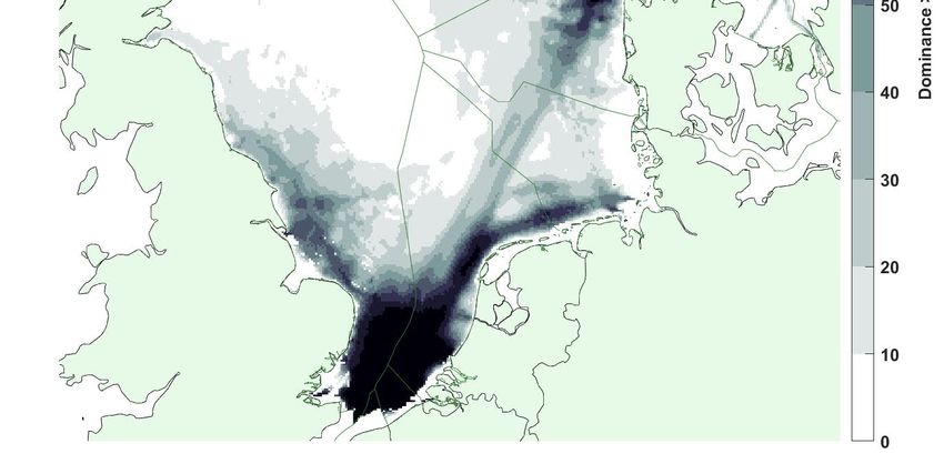
INTERREG North Sea Region
                                                                                                             Jomopans

a combination) in a 1:1 way. If the noise increases with 1 dB, signal to noise ratio decreases with 1 dB.
The consequence of this is illustrated in Figure 2. If we consider for example the hypothetical situation
in Figure 2B, where an animal hears the call of a conspecific with a signal to noise ratio of 37 dB, this
may be sufficient for the receiver not only to detect the call, but also extract the information required for
communication (such as direction to the call, identity of the caller and perhaps intention of the caller,
the ‘message’ if you like). If ambient noise increases, as in Figure 2C, the signal to noise ratio
decreases to 7 dB, which may still be sufficient for detection of the signal, but probably not enough for
efficient communication. The receiver is now beyond the maximum communication range and will have
to move closer to the sender in order to restore communication. Signal to noise ratio and maximum
communication range are intimately linked: if SNR goes down, so does the maximum communication
range, all other factors kept constant.2

                                 A                                     B                                      C

                                 D                                     E                                     F

G

Figure 2: Illustration of masking with a fictive example, showing different conditions of natural ambient noise and
ship noise. Each panel represents conditions at one distinct instant in time. Assume an animal calling as loud as it
can in the frequency bands between 63 Hz and 160 Hz and a receiving animal some distance away, with an
audiogram given by the blue line and natural ambient noise given by the orange line. A) Very low natural ambient
noise level. Hearing is limited by the audiogram, indicated by the signal-to-noise ratio (SNR, orange arrow). B)
Elevated natural ambient noise level. Hearing is masked by the natural ambient and SNR smaller. C) High natural
ambient noise level. SNR is low and communication more difficult than in B. D) Low level of ship noise added. Total
noise elevated above natural ambient. Relative to situation in B, SNR is decreased with 7.8 dB, which is the
difference between purple and orange lines and termed the excess level. E) Higher ship noise means higher excess
and lower SNR. F) If natural ambient is high, the influence of ship noise almost zero (excess level 1.8 dB, SNR
almost the same as in C). G) Very high ship noise level and consequently very poor SNR.

The examples serve to introduce the fundamental metric excess level and illustrates some of the
features that make it useful in assessment of anthropogenic noise:
     1. Excess level is related to signal to noise ratio and thereby to maximum communication range.
         If excess increases, maximum communication range decreases, everything else being equal.

2
  This does not mean it is the only important factor. Many other factors, including sound propagation properties and
the ability of the sender to change the structure of the call to improve reception by the receiver, affects the signal to
noise ratio of the receiver. Although this complicates matters considerably when dealing with actual studies of
masking, it does not affect the fundamental relationship between signal to noise ratio and maximum communication
range.

                                                                                                                  9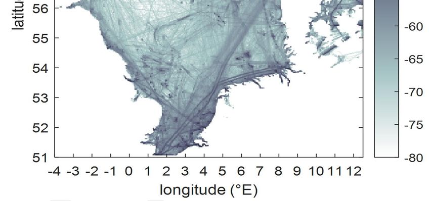
INTERREG North Sea Region
Jomopans

      2.    Excess level is always relative to the natural ambient noise, which means that it expresses the
            difference between actual conditions and what they would have been in the absence of
            anthropogenic sources.
      3.    Excess level is fundamentally an instantaneous measure, which changes from minute to
            minute as the noise conditions change.
      4.    Excess level is independent of the actual signal used for communication. This means that it
            can be estimated without any knowledge of the signal to noise ratio required for
            communication or the actual maximum communication range.

The fundamental relationship is that if excess increases, the conditions for acoustic communication
deteriorate and this deterioration is due to the anthropogenic noise, not natural fluctuations in ambient
noise.

1.3        Stepwise approach to monitoring and assessment

Figure 3: Framework ambient sound indicators (from Van Oostveen et al, 2020)

      10
INTERREG North Sea Region
Jomopans
Table 1: Framework of indicator ambient sound based on the candidate indicator of ambient noise (EIHA 2019) with
minor changes for ICG Noise 2019.
Activity / task Description of activity
The human activities that generate low-frequency continuous sound
need to be evaluated. Sources of this information are AIS (for
1. Collect information on
shipping intensities), VMS (for fishery activities) and the OSPAR
human activities
impulsive noise register (for other sources of noise). These data need
to be obtained with a temporal resolution of 1 hour maximum.
Acoustical properties of most of the sources are not available in a
sufficient detail. Literature can provide statistical proxies for these
properties. Jomopans has developed in co-operation with JASCO
2. Collect acoustic
and the ECHO project (Port of Vancouver) a model for ship noise
properties of the sources
source levels, RANDI3.1c . It is important to continuously improve the
knowledge of the source properties. These models can be verified
using field measurements where required.
Bathymetry and properties of the sea bottom (composition) are
3. Collect physical
important for the numerical modelling of sound propagation. These
properties of the
parameters can be considered static. (Meteo) parameters, like wind,
environment
rain, current, temperature, isoclines, salinity are dynamic.
Through acoustical propagation modelling sound scape maps (sound
pressure level as well as background level) will be calculated as
defined in the indicator metric.
4. Calculate soundscape
Acoustical models for sound from natural sources are available and
and excess level maps
being evaluated. Propagation models for sound propagation of
various sound sources can be chosen.
From these excess level maps and dominance maps can be derived.
At a number of measurement stations the soundscape is monitored
5. Measure long term
on an ongoing basis. From these measurements statistical
acoustical parameters at
parameters of the SPL can be derived. The measurements can be
a number of stations
used to validate the modelling as well as for other purposes.
6. Evaluate the Using the sound scape maps and the measurements a validation is
soundscape maps and performed, and confidence maps will be produced which indicate
produce confidence maps where there is greater or lesser confidence in the model predictions.
7. Specify estimated Use density estimation data if available and appropriate, otherwise
animal density or habitat use areas (e.g. habitat quality mapping, MPA, Spawning grounds,
area of indicator species etc.).
8. Compute exposure/risk Including quantitative assessment of confidence in the risk values
map by combining 6 and derived.
7
9. Compute exposure/risk A risk indicator must be computed for each relevant region, that can
indicator(s) be assessed against a GES criterion.
11INTERREG North Sea Region
Jomopans
2 Stepwise assessment
2.1 Step 1-3. Collect information on human activities, source properties and
environmental properties
Various input data need to be collected annually, to inform the sound propagation modelling. These
data involve the actual human activities, that produce continuous sound, and environmental data.
The use of these data are described in the Jomopans report on modelling (De Jong et al, 2021).
Under the assumption that ships and wind are the primary driving sources for continuous sound.
Source models for ships and wind.
2.1.1 AIS and VMS
Figure 5: AIS and VMS density map after corrections for missing data.
AIS is the main source of information on shipping activities. AIS is designed to service the shipping
industry and shipping traffic management. The use of AIS as input for underwater noise modelling is
new and it proved various improvements were needed on the obtained AIS data.
VMS is a system for the fisheries and gives additional information on activities of fishing ships. Access
to VMS data is in some countries very limited.
The initial data delivery proved to be incomplete and subsequent data deliveries were needed.
Integration of VMS data improved the density maps for fishery vessels.
The resulting maps still showed gaps and detailed analysis proved that a further interpolation of
shipping tracks was needed to end at the final map shown in figure 5.
De Jong et al (2021) discusses the AIS analysis and interpolation of AIS data.
Note that there are more sources of continuous noise than shipping. In most areas in the North Sea
shipping is dominant. Further work is needed to include other sources, like operational wind farms.
12INTERREG North Sea Region
Jomopans
2.1.2 Bathymetry
Figure 6: Bathymetry of the North Sea (Source EMODNET Bathymetry)
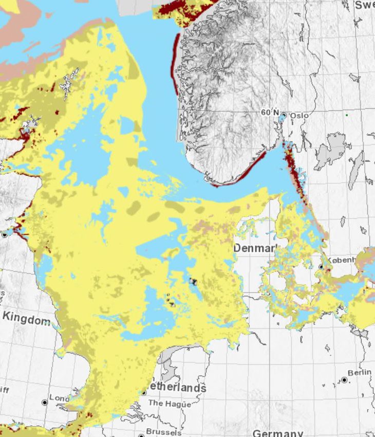
2.1.3 Sea bottom composition
Figure 7: Sea bottom composition (source EMODNET Geology).
13INTERREG North Sea Region
Jomopans
2.1.4 Others
2.2 Step 4. Modelling soundscape maps
The soundscape maps will be generated through sound propagation modelling. In the Jomopans
modelling guidelines report the method is described on how to make soundscape maps.
More details on the modelling method can be found in De Jong et al (2021).
Different indicator species are sensitive in different parts of the frequency spectrum. This must be
included in the assessment by selection of an appropriate frequency band for the assessment and can
be narrow band (1/3 octave) or wider. The Jomopans tool currently allows assessment for the MSFD
bands 63Hz and 125 Hz, and decadal bands 20-200 Hz, 200H-2 kHz and 2 kHz-20 kHz. A broadband
level (20 Hz-20 kHz) is also supplied, but for reference only, as the broadband level will be almost
completely dominated by the lower frequencies and therefore provide little additional insight compared
to the other bands. Selection of appropriate band for assessment is beyond the scope of this report,
however. It is simply assumed that the band selected is relevant to the indicator species.
Jomopans calculated the soundscape maps for the 63 Hz, 126 Hz and … Hz 1/3-octave bands. In this
assessment the maps of the 126 Hz 1/3-octave and are presented. This band contains the major noise
levels caused by shipping noise.
Figure 8: Median Background Sound Level 126 Hz band (wind)
· Remarks on the used model to calculate the background sound levels.
14INTERREG North Sea Region
Jomopans
Figure 9: Median Sound Pressure Level by shipping, 126 Hz band.
Figure 10: Median Excess Level, 126 Hz band.
To be included:
15INTERREG North Sea Region
Jomopans
· Topic for policy decisions:
o Shipping lanes
o Spatial variations
o Low noise zones
o Silent ships
2.3 Step 5. Measure long term acoustical parameters at several stations
Ambient sound data will be obtained by hydrophone measurements at selected locations within the
area of the North Sea. In the Jomopans measurement-guidelines report (Fischer et al, 2021) the
method is described on how to conduct measurements of ambient sound.
The basic role of measurement stations in the monitoring programme is the local validation of the
modelling and production of uncertainty maps. In addition, measured data of noise from individual
ships are important in the work of studying different parameters such as ship categories, age and
speed and other, on the radiated sound. Apart from this also other considerations play a role, such as a
policy choice to have more stations or the stations to serve other applications.
Measurements are a national responsibility and also the choice of measurement setup is. The costs
can vary depending on this choice. In this report we give some estimates of these cost based on the
Jomopans experience to help the national authorities to make choices and to prepare budget
estimates.
Figure 11: Underwater sound monitoring locations of the JOMOPANS-project. Monitoring locations are depicted
with consecutively numbered circular markers (colours represent the different partners/countries). The green
coloured area indicating the project area. It should be noted that one monitoring station (13-NO-LOV) is not shown
on the map. This station serves as a reference station (very low shipping) and is located in the northern area of
Norway and outside of the specific project region.
16INTERREG North Sea Region
Jomopans
Table 2: Available hydrophone data from 2019
To be included:
· Spatial distribution of stations
o Improvements advised based on results modelling
· Results from measurements
· Multiple use of measurements for underwater noise (memo Mathias)
2.4 Step 6. Confidence maps
Using the sound scape maps and the measurements a validation is performed and confidence maps
will be calculated.
· Use measurements at different locations (with different sediment type, water depth,
temperature and ocean condition).
· Comparison of measurements with models must be executed using statistical techniques (to
be determined).
· Identify environmental parameters which are more important than others. For example:
sediment grainsize.
· Make an estimate for the uncertainties there are, based on measurements we have.
Prediction at site level. Do we have enough data points to do the statistics? This can be
figured out when doing it.
Confidence in the predictions is an important factor for policymakers.
The work on the comparison of modelled maps and measurement data is progressing and cannot yet
be reported. Results are expected in April 2021. See Merchant et al (2021).
17INTERREG North Sea Region
Jomopans
2.5 Assessment of continuous noise
Underwater noise can vary greatly in time and space. Ultimately the aim of an assessment is to qualify
for an assessment area whether the Good Environmental Status (GES) is reached or not.
The maps presented in section 2.2 of this report display the spatial variation of the soundscape and the
temporal variation are reduced by taking the median value for the evaluation period (one year).
A dominance map aims to make the temporal variations more visible. Dominance is the percentage of
time that the excess level is higher than a certain cutoff level. In figure 12 the dominance is shown for a
cutoff level of 20 dB. Annex A gives a more detailed description of the Dominance.
Figure 12: Dominance maps for a cutoff level of 20 dB of the Excess Level.
Excess and dominance are derived for individual positions (grid cells), as illustrated in the maps in the
previous figures.
For an assessment period (one month) the excess level can be characterized by percentiles, such as
the 50th percentile (median) in figure 10. Dominance is also calculated from the individual snapshots,
as described above, but in contrast to the excess level there is only a single dominance value
associated with each grid cell (figure 12). This map represents the anthropogenic pressure on the
assessment area. Where dominance is high (English Channel, NW corner of Denmark), the current
condition is dominated by ship noise most of the time, whereas in areas with low dominance (Dogger
Bank, shallow parts of Kattegat), the current condition is within 20 dB of the reference condition most of
the time.
The dominance across the entire assessment area can be analysed quantitatively by means of the
pressure curve, which is constructed from the distribution of dominance over the entire MRU (Figure
14). The dominance in the example from the entire North Sea shows that most of the grid cells of the
North Sea have low dominance, indicated by the median dominance of 22% (white bars). On the other
hand, 10% of the area has a dominance of 66% or higher (dark grey bars) and about 2% of the grid
cells have a dominance of 100%, which indicates that current conditions are always elevated with 20
dB or more above the reference condition. This is reflected in the pressure curve (Figure 14B), which is
constructed from the distribution by a cumulative sum of the affected area from the high end of the
distribution (right in Figure 14A). All pressure curves must start in (0,100) as no part of the area can
have a dominance above 100 %. Likewise, they all end in (100, 0), as 100 % of the area must have a
dominance of at least zero. The part of the curve between these anchor points carries information
about the pressure on the assessment area. Figure 14C shows two idealized pressure curves to
illustrate interpretation of the curve. The blue curve represents an area with little anthropogenic noise,
18INTERREG North Sea Region
Jomopans
which means that most of the assessment area has low dominance. The median dominance is 5%,
while only 2% of the area has a dominance of 50% or more (both indicated as blue circles). The orange
curve represents an area heavily affected by ship noise. The median dominance is 95%, while only 2%
of the area has a dominance lower than 50% (both indicated by orange circles). Thus, the higher
towards the upper right corner, the more affected the area is by anthropogenic noise, and vice versa:
the further towards the lower left corner, the less affected the area is.
A B C
Figure 14. Distribution of dominance and the pressure curve. A) Distribution of dominance in grid cells of the
assessment area (Figure 2D). Most grid cells have low dominance. The white bars indicate the median: half of the
area has a dominance of 22% or less, whereas the dark grey bars indicate the upper 10th percentile: 10% of the
area has a dominance of 66% or higher. B) The pressure curve, derived from the distribution in A by summing the
bars from the high end. The dark grey lines thus represents the upper 10th percentile and the light grey lines the
median. C) Two idealized pressure curves, illustrating curves from an area less affected by ship noise (blue) and an
area heavily affected by ship noise (orange).
2.5.1 Assessment selected areas
For the assessment and one or more assessment areas have to be chosen. In the above the pressure
function for the whole North Sea region was used. In this section we show as an example the pressure
functions for six subregions based on OSPAR assessment areas (Northern North Sea, Southern, North
Sea, Doggersbank, Norwegian Trench, Skagerak and Kattegat) as depicted in figure 15.
The individual pressure curves are shown in Figure 16 and they illustrate two important features of the
curves, besides the fact that they group into two groups of three areas each. The black curve for the
Southern North Sea (SNS) has a pronounced ‘bump’ in the upper left corner. This indicates areas with
chronic exposure: about 10% of the MRU has a dominance close to 100%. This is the influence of the
very intense shipping in the English Channel and along the coast of Belgium (compare with the
pressure map in Figure 9). The light blue curve for the Northern North Sea (NNS) has a similar ‘bump’,
but in the lower right corner. This indicates that the pressure is widespread: 90% of the area has a
dominance of 10% or more, but only about 10% of the area has a dominance of more than 50%. The
shape of the curve and the degree of asymmetry around the positive diagonal therefore carries
additional information about the spatio-temporal characteristics of the anthropogenic noise in the MRU.
Figure 15: Assessment areas.
19INTERREG North Sea Region
Jomopans
SNS
NOR
SKA
NNS
KAT
DOG
Figure 16: Pressure functions for the assessment areas in figure 15
The choice of assessment areas can be made on various grounds and needs further discussion.
Other possible choices can be based on national boundaries or marine protected areas.
The pressure curve itself provides a very condensed expression of the conditions in the area under
assessment, with respect to the relationship between natural ambient noise (the reference condition)
and the current condition. It cannot be used directly to assess GES status, however, because a one-
dimensional number is required for this. However, the area below the pressure curve can serve this
function as a one-dimensional pressure index. This pressure index lies between 0 and 1, with 0 by
definition being GES, as this means that the reference condition is attained everywhere, all the time.
On the other hand, a value of 1 represents a condition, which intuitively cannot be GES: Current
condition is above the high-risk level everywhere, all the time. The threshold between GES and not-
GES thus must be some number between 0 and 1.
There is no method available to derive the threshold from first principles, however. To do this requires
a level of quantitative understanding of how ship noise affects populations of indicator species through
masking of communication, which we do not have and is unlikely to obtain in near future.
Figure 16: Pressure indices corresponding to the pressure function in figure 15 for the 6 assessment areas of
figure 14
20INTERREG North Sea Region
Jomopans
3 Discussion
The pressure index (area below the pressure curve) for the six MRUs are shown in figure 15. As
evident from the pressure curves directly, the MRUs group into three areas with a high pressure index,
around 0.5, and three with a lower index, around 0.2. As stated above, these numbers do not by
themselves indicate whether GES is attained in the MRU or not, as there is no way to derive a
threshold without additional information about the MRUs and in particular the indicator species in the
MRUs. The suggested approach to establishing a threshold for GES based on the pressure index is
therefore to assess the individual MRUs by expert judgement. If the MRUs can be ranked according to
what their GES status is judged by expert opinion, this ranking can be compared with the index. If the
index works as intended, there will be a strong correlation between assessed status and the pressure
index. This relationship can then be reversed to establish the GES threshold. Given there is such a
strong correlation for the North Sea MRUs (which has not yet been established), three different
outcomes are possible:
· All MRUs are assessed as being in GES. The threshold for GES must be below the lowest
value: 0.17 (Kattegat)
· All MRUs are assessed as not being in GES. The threshold for GES must be above the
highest value: 0.51 (Norwegian Trench)
· Kattegat, Dogger Bank and Northern North Sea assessed as being in GES, Southern North
Sea, Skagerrak and Norwegian Trench as not being in GES. The threshold must be between
0.24 (Northern North Sea) and 0.5 (Skagerrak).
Thus, by computing the pressure index for a large number of MRUs and compare with their expert
judged GES status, the value of GES threshold can be gradually narrowed in and established. It is
clear that there could be regional differences, which means that the process may ned to be repeated
for each region, leading to regionally specific threshold values.
21INTERREG North Sea Region
Jomopans
References
De Jong, C.A.F., (2021) WP4 final report. Modelling. Report of the EU INTERREG Joint Monitoring
Programme for Ambient Noise North Sea (JOMOPANS), March 2021
Fischer, J-G., Kühnel, D., Basan, F. (2021) WP5 final report. Measurement guidelines. Report of the
EU INTERREG Joint Monitoring Programme for Ambient Noise North Sea (JOMOPANS), March 2021
Merchant, N. D., Faulkner, R. C., & Martinez, R. (2018). Marine noise budgets in practice.
Conservation Letters 11(3), e12420. http://dx.doi.org/10.1111/conl.12420
Merchant, N. D., Farcas, A., Powell, C. F. (2018) Acoustic metric specification. Report of the EU
INTERREG Joint Monitoring Programme for Ambient Noise North Sea (JOMOPANS).
Merchant, N.D., Putland, R., Farcas, A. (2021) Validation report. Report of the EU INTERREG Joint
Monitoring Programme for Ambient Noise North Sea (JOMOPANS), April 2021
Nikolopoulos A., Sigray P., Andersson M., Carlström J., Lalander E. (2016) BIAS Implementation Plan -
Monitoring and assessment guidance for continuous low frequency sound in the Baltic Sea, BIAS
LIFE11 ENV/SE/841. Available from www.bias-project.eu.
Snoek, R. (2015) Ambient noise monitoring strategy and joint monitoring programme for the North Sea
– Part 1: Monitoring strategy ambient noise, Arcadis-report
Van Oostveen, M., Barbé, D., Kwakkel, J. (2020) Proposal assessment framework - OSPAR candidate
indicator ambient underwater sound, Report Royal Haskoning DHV, November 2020.
Wang, L, Ward, J. and Robinson, S. (2019) Standard for Data Processing of Measured Data. Report of
the EU INTERREG Joint Monitoring Programme for Ambient Noise North Sea (Jomopans), February
2019 (draft).
22INTERREG North Sea Region
Jomopans
Annex A Dominance
Masking is a naturally occurring phenomenon, as explained above, which means that there is nothing
fundamentally different for the animal in being masked by a heavy rain shower or a passing ship. What
the presence of ship noise changes is the time available for communication. This means that it is
relevant to assess how often the ship noise dominates over the natural ambient and thereby limits
communication. As masking requires the masking noise to occur simultaneously with the signal of
interest, this comparison should be done on a very fine time scale. This can be done by evaluating the
dominance, which expresses the percent of the assessment period (for example one month) where
ship noise is the limiting factor for communication rather than natural ambient. Dominance should be
calculated based on individual snap shots
ℎ ℎ >
= ∙ 100%
ℎ
I.e. the ratio of snapshots in which the Excess level is above some cut-off value (Lcutoff)3. This cut-off
value can be interpreted in two different ways, either as a level above which some undesired effect
(masking) is very likely to occur, or as an arbitrarily chosen value maximizing the dynamic range of the
dominance parameter. Both interpretations are valid and not mutually exclusive.
If Lcutoff is interpreted as a threshold level for masking then it should be selected as a level indicating
significant deterioration of conditions for communication relative to the reference condition (natural
ambient noise dominating). Tentatively, Lcutoff is set to 20 dB, which means that conditions are
considered deteriorated due to the ship noise if the excess level is 20 dB or higher, equal to a decrease
in signal to noise ratio of 20 dB or more, relative to the reference condition. Under simplifying
assumptions of spherical spreading loss of the communication signals and insignificant absorption4,
this translates into a decrease in maximum communication distance by 90%. The selection of Lcutoff can
also be based on pragmatic considerations of the dynamic range of the dominance. If , Lcutoff is too low,
then dominance will approach 100% in areas with many ships, making it difficult to resolve differences
between areas. Similarly, if Lcutoff is too high, dominance will be close to 0% in areas with little shipping,
also preventing differences between these areas to be resolved. A pragmatic compromise balancing
the two is therefore required. The tentative choice of 20 dB appears to achieve this, as will be
illustrated below.
3
Lcutoff must not be confused with the threshold for GES assessment.
4
This will likely be a good approximation for example for fish communicating over relatively small distances, but not
for baleen whales communicating across ocean basins. The assumption of spherical spreading is not important for
the index, however.
23You can also read