Control of a Lifted H2/N2 Flame by Axial and Flapping Forcing: A Numerical Study
←
→
Page content transcription
If your browser does not render page correctly, please read the page content below
Control of a Lifted H2/N2 Flame by Axial and Flapping Forcing: A Numerical Study Artur Tyliszczak ( atyl@imc.pcz.pl ) Częstochowa University of Technology Agnieszka Wawrzak Częstochowa University of Technology Research Article Keywords: large eddy simulation (LES), nozzle transforms, apping direction, uctuations intensifying, non-excited ame Posted Date: September 15th, 2021 DOI: https://doi.org/10.21203/rs.3.rs-858118/v1 License: This work is licensed under a Creative Commons Attribution 4.0 International License. Read Full License

Control of a lifted H2/N2 flame by axial and flapping
forcing: a numerical study
Artur Tyliszczak1,* and Agnieszka Wawrzak1
1 Facultyof Mechanical Engineering and Computer Science, Czestochowa University of Technology, Al. Armii
Krajowej 21, 41-201 Czestochowa, Poland
* atyl@imc.pcz.pl

ABSTRACT

The large eddy simulation (LES) method combined with the Eulerian stochastic field approach has been used to study excited
lifted hydrogen flames in a stream of hot co-flow air in a configuration closely corresponding to the so-called Cabra flame. The
excitation is obtained by adding to an inlet velocity profile three types of forcing ((i) axial; (ii) flapping; (iii) combination of both)
with amplitude of 15% of the fuel jet velocity and frequency corresponding to the Strouhal numbers St = 0.30, 0.45, 0.60 and 0.75.
It is shown that such a type of forcing significantly changes the lift-off height (Lh ) of the flame and its global shape, resulting in a
flame occupying large volume or the flame, which downstream the nozzle transforms from the circular one into a quasi-planar
flame. Both the Lh and their spreading angles of the flames were found to be a function of the type of the forcing and its
frequency. The minimum value of Lh has been found for the case with the combination of axial and flapping forcing at the
frequency close to the preferred one in the unexcited configuration. The impact of the flapping forcing manifested through a
widening of the flame in the flapping direction. It was shown that the excitation can significantly increase the level of the velocity
and temperature fluctuations intensifying the mixing process. The computational results are validated based on the solutions
obtained for a non-excited flame for which experimental data are available.

Introduction
Intensive research on applications of active flow control methods was initiated by a famous work of Crow and Champagne1
concerning a round jet. Applying a low amplitude excitation (forcing) being a sinusoidal function of time they observed that
for some range of frequency the jet behaviour significantly changes. The turbulence intensity level expressed in terms of the
velocity fluctuations increased, and moreover, its profile along the jet axis was characterised by a distinct local maximum at a
distance of approximately eight nozzle diameter from the nozzle exit. Such a behaviour was never reported before and did not
occur in natural jets. It turned out that applying a relatively simple control technique one may change the flow dynamics to the
extent incomparably larger to an energy input needed to introduce the excitations. These findings stimulated very extensive
analyzes of various excitation types including axial, flapping and helical forcing modes2–4 , and their combinations. Recent
LES (Large Eddy Simulations) and DNS (Direct Numerical Simulations) works of Tyliszczak A.5, 6 and Gohil et al.7 showed
that for carefully selected frequencies of combined axial and helical excitation one can obtain multi-armed jets, i.e., the jets
characterized by 5, 7 or 11 or even 20 separate branches, closely reminding the blooming jets reported by Reynolds and
Parekh8 . Without doubts, the active flow control methods are superior compared to the passive methods relying on optimization
of a flow domain for particular flow regimes. Mainly, because their driving parameters (the excitation amplitude/frequency,
spatial distribution, etc.) can be dynamically adapted to changing flow conditions, e.g., increasing/decreasing inlet velocity or
temperature. The passive methods do not allow for such freedom, yet, from the point of view of the working costs, they are
certainly cheaper as they do not need additional energy to operate.
    The findings on the active control techniques quickly translated to combustion science where they have been the focus of
interest since the early 1990s.9, 10 . Regarding the fundamental problems the attention is very often paid to jet-type flames in
which the mechanical or acoustic forcing acts as a source of external excitation. The former is usually introduced by specially
designed nozzle tips with magnetic or piezoelectric actuators11, 12 . The acoustic excitation is more often used and is added
by loudspeakers mounted upstream of the nozzle exits13–17 . The influence of this type of excitation on reduction of pollution
emissions in a lean premixed lifted flames and flame stability was demonstrated by Chao et al.13, 14 , among others. Focussing
on stability issues, they found that the excitation significantly alters the flame dynamics and can be used as a "tool" suppressing
or amplifying the stabilization process. Abdurakipov et al.15 demonstrated that in comparison to natural flames the excitation
ensures stable combustion regimes and visibly shifts the blow-off limits. A research on an excited lifted non-premixed flame
in a hysteresis regime, i.e., when depending on initial conditions a flame can be attached to a nozzle or remain lifted for the
same fuel velocity, was performed by Demare and Baillot16, 17 . It was shown that, by changing the amplitude and frequency of
excitation one can enhance the combustion process or produce large fluctuations, and thus, weaken the flame stability. Kozlov
et al.18 analyzed micro-flames in the field of transverse sound waves. They found that the excitation can flatten the round flames
and transform them to nearly plane flames. Surprisingly, for particular forcing frequencies the excitation led to a splitting of the
flame into two separate branches in a very similar way as observed for bifurcating non-reacting, constant density jets8 . More
recently, the occurrence of the bifurcating phenomenon in flames was reported in numerical studies of Tyliszczak19 focused on
a low Reynolds number hydrogen flame. Application of only the flapping excitation caused that the flame changed its initial
circular shape into the planar one with two co-existing separate arms. Moreover, for some range of the excitation frequency, a
triple-flame occurred.
     As discussed above, the excitation can alter the flame dynamics and influence the pollution emission. In the present work
we focus on the global impact of the excitation on the flame by applying three different excitation types: (i) axial (ii) flapping;
(iii) axial plus flapping with different forcing frequencies. The basic flow configuration closely corresponds to the so-called
Cabra flame20 at the Reynolds number equal to 23600. We apply LES method in combination with the Eulerian Stochastic
Field (ESF) approach21 for the combustion modelling. There are no experimental results for the excited Cabra flame, and hence,
the credibility of the obtained results is proven by comparison with the measurements data available for the non-excited flame.
The present research is an exploratory numerical study in which we assess large-scale effects of the excitation, i.e., the change
of the lift-off height or the change of the size and shape of the flame.

Mathematical approach
We consider a low Mach number reacting flow for which the continuity, Navier-Stokes and transport equations of scalars within
the framework of the LES method are defined as:
      ∂t ρ̄ + ∇ · (ρ̄e
                     u) = 0

      ρ̄∂t ue + (ρ̄e      e + ∇ p̄ = ∇ · τ + τ SGS
                   u · ∇) u
                                                                                                                                 (1)
                   u · ∇Yeα = ∇ · ρ̄ Dα + DSGS
      ρ̄∂t Yeα + ρ̄e                          α     ∇Yeα   + ρ ẇα

      ρ̄∂t e      u · ∇e
            h + ρ̄e    h = ∇ · ρ̄ D + DSGS ∇h

where the bar and tilde symbols denote filtered quantities. The variables in Eqs. (1) are the velocity vector u, the density ρ, the
hydrodynamic pressure p, the species mass fractions Yα and enthalpy h. The subscript α represents the index of the species
α = 1, . . . , N-species. The quantities τ and Dα , D are the viscous stress tensor and mass and heat diffusivities. The sub-filter
tensor is given by τ SGS = 2µt S, where S is the rate of strain tensor of the resolved velocity field and µt is the sub-filter viscosity
modelled as in22 . The sub-filter diffusivities in the species and enthalpy transport equations are computed as DSGS = µt /(ρ̄σ )
where σ is the turbulent Schmidt or Prandtl number assumed equal to 0.723 . The set of equations (1) is complemented with the
equation of state p0 = ρRTe with p0 being the constant thermodynamic pressure and R is the gas constant.
    The chemical source terms ρ ẇα represent the net rate of formation and consumption of the species. A highly non-linear
nature of this term means that sub-grid fluctuations cannot be ignored. In the present work the scalar equations (species and
enthalpy) are replaced by an equivalent evolution equation for the density weighted filtered PDF function, which is solved
using the stochastic field method proposed by Valiño21 . Each scalar φ̃α is represented by 1 ≤ n ≤ Ns stochastic fields ξαn such
                    Ns
that φ̃α = 1/Ns ∑n=1    ξαn . The stochastic fields evolve according to:
                                               √
      dξαn = − u
               e · ∇ξαn dt + ∇ · (Γ ∇ξαn ) dt + 2Γ ∇ξαn · dW
                                                                                                                                   (2)
                    −1
             − 0.5τSGS    ξαn − φ̃α dt + ẇα (ξαn )dt

where the total diffusion coefficient is defined as Γ = Dα + DSGS
                                                              α     , the micro-mixing time scale equals to τSGS = ρ̄∆2 /(µ + µt )
              1/3
with ∆ = Volcell being the LES filter width and dW represents a vector of Wiener process increments different for each field.
Following Jones and Navarro24 eight stochastic fields have been used. The test computations performed with sixteen fields did
not show any substantial changes in the flames dynamics.

Numerical method
We apply an in-house numerical code (SAILOR) based on the projection method for pressure-velocity coupling25 . The time
integration is performed by means of an operator splitting approach where the transport in physical space and chemical
terms are solved separately. The convective and diffusive parts of the governing equations are advanced in time using a
predictor-corrector technique with the 2nd order Adams-Bashforth / Adams-Moulton methods. The chemical reactions are
computed using CHEMKIN interpreter. In the present study analyze the hydrogen combustion using a detailed mechanism of

                                                                                                                                   2/10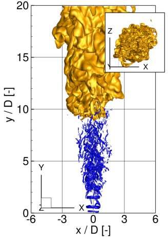
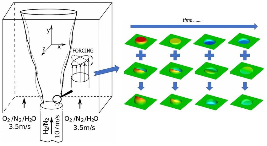
Figure 1. Schematic view of the computational domain with axial velocity iso-surface showing the time evolution of axial and
flapping forcing
                                                           .

Mueller26 involving 9 species and 21 reactions. The reaction terms are stiff and therefore they are integrated in time applying
the VODPK27 solver that is well suited for stiff systems. The spatial discretization is performed on half-staggered meshes
applying the 6th order compact difference approximation for the Navier-Stokes and continuity equations25, 28 . The convective
terms in the stochastic field equations equations are discretized applying TVD scheme with van Leer limiters. The applied code
has been thoroughly verified in previous studies19, 25, 29–31 and it turned out to be very accurate.

Computational configuration
The basic flow configuration analyzed in this study corresponds to the so-called Cabra flame20 , which we modify by adding the
excitation at the nozzle exit. A schematic view of the computational geometry is shown in Figure 1. It is a rectangular box with
dimensions Lx × Ly × Lz = 14D × 30D × 14D, where D = 0.00457 m is the nozzle diameter. The injected fuel (XH2 = 0.254,
XN2 = 0.746) has the temperature Tfuel = 305 K and the bulk velocity U j = 107 m/s. Outside of the fuel nozzle there is a
hot (Tcf = 1045 K) co-flowing stream of the hydrogen combustion products (XO2 = 0.147, XH2O = 0.1, XN2 = 0.753) with
the velocity Ucf = 3.5 m/s. The excitation (forcing) is introduced as a component of the velocity prescribed at the inlet as
u(~x,t) = umean (~x) + uturb (~x,t) + uexcit (~x,t), where umean (~x) is the mean velocity profile corresponding to the fully developed
pipe flow (1/7 profile) and uturb (~x,t) = 0.05U j represents turbulent fluctuations computed applying a digital filtering method
proposed by Klein et al.32 . This method guarantees properly correlated velocity fields which reflect realistic turbulent flow
conditions. The forcing component uexcit (~x,t) is added to the streamwise velocity only and it is defined as:
                                                           πx
       uex (~x,t) = Aa sin (2π fat) + A f sin 2π f f t sin
                    |     {z       } |                {z      D }                                                                    (3)
                    Axial forcing
                                          Flapping forcing

which is the superposition of axial and flapping forcing term with amplitudes Aa and A f and frequencies fa and f f . Figure 1
shows a sample temporal evolution of the velocity disturbance when both forcing terms are applied. The Strouhal numbers
corresponding to fa and f f are defined as Sta = fa D/U j and St f = f f D/U j . In this study we keep the amplitudes constant
and equal to Aa = A f = 0.15U j and we analyze dependence of the flame behavior on the forcing frequency assuming
Sta = 0.30, 0.45, 0.60, 0.75 and St f = Sta /2 for which the strongest effect of the flapping term was observed8, 19, 33 . We
consider three possible combinations of the forcing: (i) the axial only - the cases denoted as ASt , where the subscript defines the
forcing frequency, e.g. A45 denotes the axial forcing with Sta = 0.45; (ii) the flapping forcing only - the cases FSt ; (iii) both
forcing turned on - the cases AFSt .

                                                                                                                                  3/10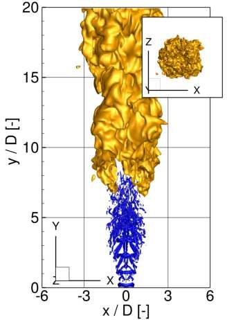
As mentioned in the Introduction section, the simulations and results discussed in this study has an exploratory character as
no experiments or numerical data are available for validation of the obtained results regarding the excited flames. Therefore the
comparison was performed only based on measurements for the original Cabra flame configuration of which a spatio-temporal
complexity is not much different from the cases with the excitation. As will be presented the agreement between the preset
results and experimental data is sufficiently good to assume that the obtained results are reliable.

Results and discussion
Three-dimensional flame behavior
The fuel issuing from the nozzle mixes with the co-flowing hot stream and auto-ignites. The ignition spots appear at the
locations of the most reactive mixture fraction ξMR = 0.053 at distances far from the inlet, i.e. y/D ≈ 20. Then, the flame
spread radially, propagates upstream and stabilizes as a lifted flame in between y/D ≈ 7.5 − 11.0 depending on the test case.
Figure 2 shows iso-surfaces of instantaneous temperature (T = 1200 K) and Q-parameter (Q = 10 s−2 ) for the cases without
the excitation and for A45 , A60 and A75 . The Q-parameter is commonly used to indicate organized vortical motion. It is defined
as Q = 1/2(Ωi j Ωi j − Si j Si j ), where Si j and Ωi j are the symmetric and antisymmetric parts of the velocity gradient tensor.
Here, it visualizes the effect of the excitation, which manifests by occurrence of toroidal vortices formed in the vicinity of the
nozzle. They mutually interact through rib-like vortices and break-up further downstream. Compared to the unexcited case (see
Figure 2a) the vortices are much more pronounced, the distances between them are dependent on the forcing frequency and
decrease with increasing Sta . One can notice that in the case A60 the jet at y/D ≈ 1.0 − 4.0 is wider than for A45 and A75 and its
shape reminds a barrel. The temperature distributions reveal that the flame lift-off height depends on the forcing frequency
and turns out to be the smallest for A60 that will be further confirmed by time-averaged results. The flame behavior changes
significantly when the flapping forcing is turned on. Figure 3 shows the results for the cases AF60 and AF75 in which the
flapping forcing causes that the toroidal vortices are tilted with respect to the axial direction. Note that this effect is noticeably
stronger for AF75 . For AF60 the tilting of the vortical rings is overwhelmed by its very strong amplification by the axial forcing
term, as will be discussed in the next sections. In both the cases, however, the rings have tendency to move alternately to the left
and right side of the domain and in effect the flames with the flapping excitation become wider in the ’x’-direction and narrower
in the ’z’-direction. In Tyliszczak A.19 it was shown that for low Reynolds number (Re = 4000) the flame can even bifurcate
(i.e. split into two separate branches), however here this phenomenon does not occur. For the present case with Re = 23600 and
relatively high level of the inlet turbulence intensity the toroidal structures are destroyed before reaching a bifurcation point that
usually is located at y/D ≈ 533 .

Effect of the excitation in spectral space
Figure 4a shows axial velocity spectrum computed based on a velocity signal recored in the axis at y/D = 3.0 for the case
without the excitation. It can be seen that there are no distinct peaks in the spectrum that could be related to the preferred mode
frequency or the parring process. Apparently, as can be seen in Figure 2a, the level of turbulence imposed at the inlet prevents
formation of strong, well defined vortical structures, which periodic occurrence would certainly manifest also in the spectrum.
Instead, only a rise of the fluctuations amplitudes at a broadband range of the frequencies is observed, which is centered around
St = 0.6. The excitation at Sta = 0.60 was chosen to match exactly this value, whereas the excitation at Sta = 0.30 corresponds
to its sub-harmonic at which the parring process could exist. Figure 4b shows the velocity spectra for the cases with the axial
forcing only. Distinct peaks corresponding to the excitation frequencies are readily seen as they are definitely larger than the
background level. The cases A45 and A75 do not show anything exceptional. The peaks related to their basic frequencies are
virtually the only ones visible. Further downstream they become wider and lower (not presented) and it seems as there are no
additional phenomena created by the forcing at these frequencies. The results for A30 and A60 are significantly different. In
the former case (green line in Figure 4b) the excitation causes intensified velocity fluctuations not only at the basic frequency
but also at its harmonic St = 0.60. The most striking difference is, however, for the case A60 for which the whole bench of
highly energetic harmonics is found. They appear as the results of interactions between subsequent vortices. These interactions
take place through the wavy shape elongated rib structures (see Figure 2c) that connects the vortex rings. One could expect
that existence of harmonics causes intensified mixing at small scales that speeds up the ignition process. The velocity spectra
obtained for the cases with the axial and flapping forcing acting together show similar features, thought, the harmonics are
much weaker. The spectra for the cases with the only flapping excitation turned on are not significantly different from the ’no
forcing’ case as in the axis locations close to the inlet the impact of the flapping should not be pronounced by definition.

Impact of the excitation on the lift-off height
The lift-off height (Lh ) of the flames is estimated based on the time-averaged results. The time-averaging procedure started
when the flames were fully developed and it lasted for the time period at least 300D/U, which was found sufficient to obtain
well convergent statistics. Figure 5 shows the contours of the time averaged OH mass fraction and temperature in the central

                                                                                                                                4/10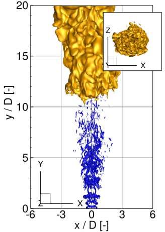
(a) no forcing                                     (b) A45

                                 (c) A60                                         (d) A75

Figure 2. Iso-surfaces of the Q-parameter (Q = 10 s−2 , blue) and temperature T = 1200 K (yellow). Subfigures show the
view of the flames from the bottom along the ‘y’ coordinate.

                                                                                                                    5/10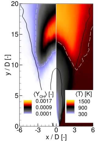
(a) AF60                                             (b) AF75

                                        Figure 3. As in Figure 2 but for AF60 and AF75 .

‘x-y’ cross-section plane. The inner black lines represent the stocihometric mixture fraction ξST = 0.476 and the outer ones
correspond to ξMR . The white dashed lines denotes the OH mass fraction equal to YOH = 2.0 × 10⁻⁴ and T = 1.01Tcf , which
are the typical criteria used to estimate Lh 34 . It can be seen that both the shapes of the flames and Lh are dependent on the
type of the excitation. The Lh was measured as the lowest point in the domain where the temperature or YOH exceeded a given
threshold. In all the cases these locations occur not in the flame axis but a few diameters off-axis. The Lh predicted based
on the temperature criterion is slightly smaller than using the OH mass fraction criterion, however, the differences are not
very significant (∆Lh < 1.0D). Worth noting is that both threshold lines predict very similar behaviour. For the case A60 in the
central part of the flame these lines are almost straight and their inclinations to the flame axis depend on the forcing frequencies
(not shown). When the flapping forcing is turned on the threshold lines become rounded. Figure 6 shows dependence of the Lh
on the forcing frequencies for all analyzed cases. For the case without the excitation Lh = 9.7D (Lh = 10D in the experiment20 ),
which visibly differ from Lh found applying the excitation. In these cases, depending on the forcing frequency and excitation
type Lh changes in the range 7.9D − 11.2D and is the lowest when the combination of axial and flapping forcing is applied.
Turning on only the flapping excitation mode causes that Lh reaches the maximum at Sta = 0.45 after which it continuously
decreases as the effect of intensified mixing of smaller spatio-temporal flow scales caused by higher forcing frequencies. For the
axial excitation, both acting solely or in the combination with the flapping mode, Lh behaves in a different manner. It reaches
the maximum at Sta = 0.75 but first it suddenly drops down for the forcing frequencies Sta = 0.45 and Sta = 0.60 for the
axial-flapping and axial modes, respectively. The occurrence of these minima is related to the appearance of the high frequency
harmonics in the spectra in Figure 4a. They have similar impact on the mixing as the increase of the forcing frequency of the
flapping excitation.

Impact of the excitation on time-averaged results
It could be observed in Figure 5 that the excitation changes not only the flames positions but also visibly influences on their
shapes and spreading angles. Compared to the cases with the axial excitation the flapping forcing makes the flame significantly
wider. Figures 7 and 8 shows the profiles of time-averaged temperature along ‘x’ and ‘z’ directions compared with the
experimental data at y/D = 1, 3, 8, 11. First, it should be noted that the present results agree well with the measurements.
The location where the fuel ignites in the shear layer (y/D ≈ 11) and the near axis temperature distributions are correctly
captured. Worth noting is the fact that in the experiment the co-flow temperature was biased by the 3% error20 that could lead

                                                                                                                              6/10
2
                               1                                                                                                  10
                          10                                                                                                                           St=0.3   0.45
                                                                                                                                                                       0.6 0.75
                                                                                                                                                                                      1.2 1.8
                                                                            St≈0.6                                                     1

                                                                                                          Amplitude of u’ [m/s]
  Amplitude of u’ [m/s]

                               0
                                                                                                                                  10                                                         2.4
                          10

                                                                                                                                       0
                           -1
                                                                                                                                  10
                      10

                                                                                                                              10-1
                           -2
                      10
                                                                                                                                                       A30             A60
                                   No forcing
                                                                                                                              10
                                                                                                                                   -2                  A45             A75
                           -3
                      10                 -1                             0                     1                                                   -1                              0                       1
                                    10                             10                    10                                                  10                              10                      10
                                                         Strouhal number                                                                                           Strouhal number
                                                              (a)                                                                                                        (b)

                                      Figure 4. Velocity spectra at y/D = 3.0 without forcing (a) and with the axial forcing (b).

                                              (a) Case A60                                        (b) Case AF60                                                                       (c) Case F60

Figure 5. Contours of the time averaged OH mass fraction and temperature in the central ‘x-y’ cross-section plane.

                                                                        12
                                                                                         A
                                                                                         AF
                                                                        11               F
                                                             Lh/D [-]

                                                                        10

                                                                            9

                                                                            8

                                                                                0.3               0.45                                     0.6                   0.75
                                                                                                         Sta [-]

                                                                                Figure 6. Lift-off height of the flames.

                                                                                                                                                                                                              7/10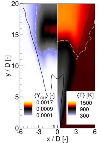
1500
                                            y/D=1                                                   y/D=3
   1200
T [K]

                                                 T [K]
        900
                                     experiment
                                     w/o excitation
        600                          A60
                                     AF60
                                     F60
        300

   1500                  x / D [-]                                              x / D [-]
                                            y/D=8                                                   y / D = 11
                                                                                            flame
   1200
T [K]

                                                 T [K]
        900

        600

        300
              0    2                 4                   00               2                    4
                        x / D [-]                                               x / D [-]
                  Figure 7. Temperature profiles for Sta = 0.60 along the ‘x’-direction.

   1500
                                            y/D=1                                                   y/D=3
   1200
T [K]

                                                 T [K]

        900
                                     experiment
                                     w/o excitation
        600                          A60
                                     AF60
                                     F60
        300

   1500                  z / D [-]                                              z / D [-]
                                            y/D=8                                                   y / D = 11
                                                                              flame
   1200
T [K]

                                                 T [K]

        900

        600

        300
              0    2                 4                   00               2                    4
                        z / D [-]                                               z / D [-]
                  Figure 8. Temperature profiles for Sta = 0.60 along the ‘z’-direction.

                                                                                                                 8/10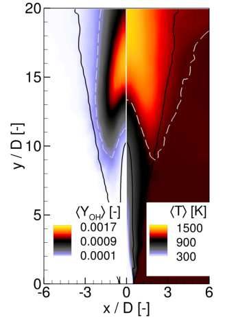
to ±15 K difference compared to the assumed Tcf = 1045 K. As observed by Navarro-Martinez and Kronenburg35 the co-flow
temperature has substantial impact on the flame stabilization height. Nevertheless, it seems that ±15 K error in Tcf has not
significant impact on the present results. Regarding the excited flames it can be readily seen that close to the inlet all profiles
(also for the case without excitation) are very similar and divergences start to be seen only downstream. The temperatures are
definitively larger in the axis for all excited cases, whereas for the cases AF their maxima move radially towards larger x/D
locations. In general, the axial excitation causes faster temperature rise, while the flapping forcing makes the temperature more
uniform along the ‘x’-direction. The profiles along the ‘z’-direction presented in Figure 8 shows that further from the nozzle
the flapping excitation can lead to 30% narrowing of the flame in respect to the ‘x’-direction.

Conclusions
The paper presented the LES studies of the H2 /N2 flame excited with the axial and flapping forcing. Correctness of the results
was confirmed by comparison with available experimental data for the unexcited case. It was found that the lift-off height of the
flame, its size and shape can be altered in a wide range depending on the type of the excitation and its frequency. Compared to
the unexcited case the lift-off height can be increased or decreased. Its minimum value has been found for the case with the
combination of both axial and flapping forcing at the frequency close to the center of the broadband frequency range regarded
as the preferred one in the unexcited configuration. The impact of the flapping forcing manifested through a widening of the
flame in the flapping direction. It was shown that the excitation can be used in advanced research on optimal control strategies.

References
 1. S.C. Crow, F.H. Champagne. Orderly structure in jet turbulence. J. Fluid Mech. 48, 547–691 (1971).
 2. I. Danaila, B.J. Boersma. Direct numerical simulation of bifurcating jets. Phys. Fluids 12, 1255–1257 (2000).
 3. C.B. da Silva, O. Métais. Vortex control of bifurcating jets: A numerical study. Physics of Fluids 14, 3798–3819 (2002).
 4. T.B. Gohil, A.K. Saha, K. Muralidhar. Direct numerical simulation of free and forced square jets. International Journal of
    Heat and Fluid Flow 52, 169–184 (2015).
 5. A. Tyliszczak. Multi-armed jets: A subset of the blooming jets. Physics of Fluids 27, 1–7 (2015).
 6. A. Tyliszczak. Parametric study of multi-armed jets. International Journal of Heat and Fluid Flow 73, 82–100 (2018).
 7. T.B. Gohil, A.K. Saha1,K. Muralidhar. Simulation of the blooming phenomenon in forced circular jets. Journal of Fluid
    Mechanics 783, 567–604 (2015).
 8. W.C. Reynolds, D.E. Parekh, P.J.D. Juvet, M.J.D. Lee. Bifurcating and blooming jets. Annu. Rev. Fluid Mech. 35, 295–315
    (2003).
 9. K.R. McManus, T. Poinsot, S.M. Candel. A review of active control of combustion instabilities. Progress in Energy and
    Combustion Science 19, 1–29 (1993).
10. A.M. Annaswamy. A.F. Ghoniem. Active control in combustion systems. IEEE Control Systems 15, 49–63 (1995).
11. Y.-C. Chao, Y.-C. Jong, H.-W. Sheu. Helical-mode excitation of lifted flames using piezoelectric actuators. Experiment in
    Fluids 28, 11–20 (2000).
12. N. Kurimoto, Y. Suzuki, N. Kasagi. Active control of lifted diffusion flames with arrayed micro actuators. Experiment in
    Fluids 39, 995–1008 (2005).
13. Y.-C. Chao , T. Yuan, C.-S. Tseng. Effects of flame lifting and acoustic excitation on the reduction of NOx emissions.
    Combustion Science and Technology 113, 49–65 (1996).
14. Y.-C. Chao, C.-Y. Wu, T. Yuan, T.-S. Cheng. Stabilization process of a lifted flame tuned by acoustic excitation. Combustion
    Science and Technology 174, 87–110 (2002).
15. S.S. Abdurakipov, V.M. Dulin, D.M. Markovich, K. Hanjalic. Expanding the stability range of a lifted propane flame by
    resonant acoustic excitation. Combustion Science and Technology 185, 1644–1666 (2013).
16. D. Demare, F. Baillot. Acoustic enhancement of combustion in lifted non-premixed jet flames. Combustion and Flame
    139, 312–328 (2004).
17. F. Baillot, D. Demare. Responses of a lifted non-premixed flame to acoustic forcing. Part 2. Combustion Science and
    Technology 179, 905–932 (2007).
18. V.V. Kozlov, G.R. Grek, M.M. Katasonov, O.P. Korobeinichev, Y.A. Litvinenko, A.G. Shmakov. Stability of subsonic
    microjet flows and combustion. Journal of Flow Control, Measurement and Visualization 1, 108–111 (2013).

                                                                                                                              9/10
19. A. Tyliszczak. LES-CMC of excited hydrogen jet. Combustion and Flame 162, 3864–3883 (2015).
20. R. Cabra, J-Y Chen, R.W. Dibble, A.N. Karpetis & R.S. Barlow. Lifted methane-air jet flames in vitiated co-flow. Combust.
Flame 143, 491–506 (2005).
21. L. Valiño. A field Monte Carlo formulation for calculating the probability density function of a single scalar in a turbulent
flow. Flow, Turbulence and Combustion 60, 157–172 (1998).
22. A.W. Vreman. An eddy-viscosity subgrid-scale model for turbulent shear flow: Algebraic theory and applications. Physics
of Fluids 16, 3670–3681 (2004).
23. Branley, N. & Jones, W. Large Eddy Simulation of a Turbulent Non-premixed Flame. Combust. Flame 127, 1914–1934
(2001).
24. W.P. Jones & S. Navarro-Martinez. Large eddy simulation of auto-ignition with a sub-grid probability density function.
Combust. Flame 150, 170–187 (2007).
25. A. Tyliszczak. A high-order compact difference algorithm for half-staggered grids for laminar and turbulent incompressible
flows. Journal of Computational Physics 276, 438–467 (2014).
26. M.A. Mueller, T.J. Kim, R.A. Yetter & F.L. Dryer. Flow reactor studies and kinetic modelling of the H2/O2 reaction.
International Journal of Chemical Kinetics 31, 113–125 (1999).
27. P.N. Brown & A.C. Hindmarsh. Reduced Storage Matrix Methods in Stiff ODE Systems. Journal of Applied Mathematical
Computations 31, 40–91 (1989).
28. S. Laizet, E. Lamballais. High-order compact schemes for incompressible flows: A simple and efficient method with
quasi-spectral accuracy. Journal of Computational Physics 228, 5989–6015 (2009).
29. A. Tyliszczak. High-order compact difference algorithm on half-staggered meshes for low Mach number flows. Computers
and Fluids 127, 131–145 (2016).
30. Wawrzak, A. & Tyliszczak, A. Implicit les study of spark parameters impact on ignition in a temporally evolving mixing
layer between h2 /n2 mixture and air. Int. J. Hydrog. Energy 43, 9815–9828 (2018).
31. Wawrzak, A. & Tyliszczak, A. A spark ignition scenario in a temporally evolving mixing layer. Combust. Flame 209,
353–356 (2019).
32. M. Klein, A. Sadiki, J. Janicka. A digital filter based generation of inflow data for spatially developing direct numerical
and large eddy simulations. Journal of Computational Physics 186, 652–665 (2003).
33. A. Tyliszczak, B.J. Geurts. Parametric analysis of excited round jets - numerical study. Flow, Turbulence and Combustion
93, 221–247 (2014).
34. Stanković I., Mastorakos E, Merci B. LES-CMC simulations of different auto-ignition regimes of hydrogen in a hot
turbulent air co-flow. Flow, Turbulence and Combustion 90, 583–604 (2013).
35. S. Navarro-Martinez & A. Kronenburg. Flame stabilization mechanism in lifted flames. Flow, Turbulence and Combustion
87, 377–406 (2011).
Acknowledgements
This work was supported by National Science Center in Poland (Grant No. 2018/31/B/ST8/00762) and statutory funds of
Czestochowa University of Technology BS/PB 1-100-3011/2021/P. The authors acknowledge the International Academic
Partnerships Programme No. PPI/APM/2019/1/00062 (NAWA), which allowed collaboration with CERFACS (France) devoted
to combustion modelling. The computations have been carried out using PL-Grid infrastructure.
Author contributions statement
A.T. is the author of the numerical code. A.T. acquired the funding for the research. A.W. performed the computations and
prepared the figures. Both A.T. and A.W. analysed the results and prepared the manuscript text.
Competing interests
The authors declare no competing interests.
Additional information
Correspondence and requests for materials should be addressed to A.T.
10/10You can also read