Sensor Fault Diagnosis Method Based on α-Grey Wolf Optimization-Support Vector Machine
←
→
Page content transcription
If your browser does not render page correctly, please read the page content below
Hindawi
Computational Intelligence and Neuroscience
Volume 2021, Article ID 1956394, 15 pages
https://doi.org/10.1155/2021/1956394

Research Article
Sensor Fault Diagnosis Method Based on α-Grey Wolf
Optimization-Support Vector Machine

 Xuezhen Cheng , Dafei Wang , Chuannuo Xu , and Jiming Li
 College of Electrical and Automation Engineering., Shandong University of Science and Technology, No. 579 Qianwangang Road,
 Qingdao 266590, China

 Correspondence should be addressed to Jiming Li; wugetongxue@163.com

 Received 19 May 2021; Revised 5 August 2021; Accepted 19 August 2021; Published 10 September 2021

 Academic Editor: Radu-Emil Precup

 Copyright © 2021 Xuezhen Cheng et al. This is an open access article distributed under the Creative Commons Attribution
 License, which permits unrestricted use, distribution, and reproduction in any medium, provided the original work is
 properly cited.

 Aimed to address the low diagnostic accuracy caused by the similar data distribution of sensor partial faults, a sensor fault
 diagnosis method is proposed on the basis of α Grey Wolf Optimization Support Vector Machine (α-GWO-SVM) in this paper.
 Firstly, a fusion with Kernel Principal Component Analysis (KPCA) and time-domain parameters is performed to carry out the
 feature extraction and dimensionality reduction for fault data. Then, an improved Grey Wolf Optimization (GWO) algorithm is
 applied to enhance its global search capability while speeding up the convergence, for the purpose of further optimizing the
 parameters of SVM. Finally, the experimental results are obtained to suggest that the proposed method performs better in
 optimization than the other intelligent diagnosis algorithms based on SVM, which improves the accuracy of fault
 diagnosis effectively.

1. Introduction historical data, rather than the exact mathematical models or
 expert knowledge.
The sensor functions as a major detection device in the With the rapid advancement of artificial intelligence (AI)
monitoring system [1–3], the detection accuracy of which technology, the AI-based diagnostic methods have attracted
will be significantly reduced by breakdown. Additionally, it much interest for research in the field of fault diagnosis. In
will affect the performance of the monitoring system and [8], a Recurrent Neural Network (RNN) is put forward to
even result in economic losses and casualties in some ex- model nonlinear systems, thus achieving fault detection and
treme cases. Therefore, it is necessary to make an accurate the isolation of sensors. A very random tree method was
diagnosis of sensor faults for ensuring that the monitoring proposed to detect and diagnose the faults in sensor net-
system can operate smoothly and reliably. works in [9], which demonstrated strong robustness for
 When the fault intensity stays low, there would be some processing the signal noise but ignored the fault diagnosis
forms of sensor failure showing similar characteristics of data for sensor nodes. In [4], a hybrid continuous density HMM-
distribution, which is a leading cause for the low levels of di- based ensemble neural networks method is applied to detect
agnostic accuracy [4]. In traditional approaches to fault diag- and classify sensor node faults.
nosis [5–7], model-based methods require the establishment of However, due to the similar distribution of some fault data,
an accurately mathematical model for the research object. In it is necessary to train a variety of classifiers for the accurate
practice, however, it is usually difficult to construct the non- classification of different faults. Furthermore, a fault diagnosis
linear system for mathematical models. With regard to method intended for chiller sensors is presented in [10], which
knowledge-based methods, they rely heavily on expert expe- not only achieves feature extraction by clustering the fault data
rience, which makes them lack adaptability when new problems but also identifies the fault types by setting the clustering
arise. Additionally, data-driven methods require the learning of indicators.
2 Computational Intelligence and Neuroscience

 Abnormal data are considered the most effective indi- there is still room for improvement in terms of the search
cators of sensor failure, which are nonlinear and enormous strategy for the GWO [24, 25]. Therefore, an improvement
and make the data-driven intelligent diagnosis method more is made to the proposed α Grey Wolf Optimization
suitable for the diagnosis of sensor fault [11–13]. Machine (α-GWO) algorithm as follows. The wolf pack is still di-
learning algorithm is a commonly used method for intel- vided into four levels, while default α, β, and δ wolves have
ligent diagnosis, including Neural Networks (NNs), Support strong search capability. Social rank is the highest in the
Vector Machines (SVMs), and so on. However, the amount population, and the remaining wolves are denoted as ω. The
of fault samples is usually limited, which leads to a poor mathematical model for finding prey is expressed as
manifestation for NN. SVM has attracted much attention follows:
due to its capability of dealing with nonlinear and small
 → → → →
sample size in fault diagnosis [14, 15], but the correct ⎧
 ⎪
 ⎪ D � C · X P (t) − X (t) ,
hyperparameters must be chosen for improved perfor- ⎪
 ⎪
 ⎪
 ⎪ → → → →
mance. Mechanism of different algorithms may be disparate, ⎪
 ⎨ X (t + 1) � X P (t) − A · D ,
and the optimization of key parameters can often improve ⎪ → (1)
 ⎪
 ⎪ → → →
the performance of the algorithm [16, 17]. Researchers have ⎪
 ⎪ A � 2a · r1 − a,
 ⎪
 ⎪
proposed or improved algorithms to solve optimization ⎩→ →
 C � 2 r 2,
problems [18–20] and achieved remarkable results, which →
gives us some inspiration to choose the appropriate where
 → trepresents the number of current
 → iterations, A and
hyperparameters of SVM. Besides, it is an effective strategy C denote the synergy
 → coefficients, X P indicates the location
to improve the accuracy of diagnosis by adopting an ap- of the prey, and X refers to the current grey wolf position,
propriate method for extracting the feature of fault data. → →
 which linearly decreases from 2 to 0, while r 1 and r 2 stand
However, conventional data feature extraction methods for the random vector in [0,1]. In α-GWO, a competitive
such as Principal Component Analysis (PCA) [21] are more relationship between the head wolves is introduced to im-
suitable for processing linear data. Also, time-domain pa- prove the global search capability. Corresponding to the
rameters can also be taken as the reference indicators for search target of the head wolves in each iteration, the fault
diagnosis, but not all of them are sensitive to all sorts of classification error is taken as the score to obtain alpha score,
failure [22]. beta score, and delta score. The head wolf level is rearranged
 In order to solve the aforementioned problems, there are a according to the fault error score, and the wolf pack position
number of solutions proposed in this paper. Firstly, multiple is updated according to equations (2)–(4):
time-domain parameters are extracted from sensor fault data, → → → →
and the Kernel Principal Component Analysis (KPCA) is ⎨ D α � C 1 · X α − X ,
 ⎪
 ⎧
conducted to perform Principal Component Analysis of the ⎪ (2)
 ⎩→ → → →
time-domain parameters. Then, some of the time-domain X 1 � X α − A 1 · D α,
parameters are refused to obtain the fusion features that can → → → →
accurately reflect the characteristics of fault. Secondly, an α Grey ⎨ D β � C 2 · X β − X ,
 ⎧
 ⎪
Wolf Optimization (α-GWO) arithmetic is proposed to achieve ⎪ → → → (3)
 ⎩→X 2 � X β − A 2 · D β,
parameter majorization for SVM. The competition mechanism
is introduced to enhance the ability of algorithm to conduct
 → → → →
search. In the meantime, the dominant position of α wolf is ⎨ D δ � C 3 · X δ − X ,
 ⎪
 ⎧
reinforced to speed up convergence in the later stage of this ⎪→ → → → (4)
 ⎩
algorithm. Finally, the samples comprised of the fusion features X 3 � X δ − A 3 · D δ,
are inputted into different diagnostic models for the purpose of →
training and testing. The experimental results are comparatively where X represents
 → → the location of the wolf pack, while D α ,
analyzed to validate the method proposed in this paper for D β , and D δ refer to the distance between the current
sensor fault diagnosis. candidate wolf and the best three wolves. When |A| > 1, the
 This paper is organized as follows. Section 2 briefly wolves are dispersed in search of prey; when |A| < 1, the
explains the improvement of GWO algorithm. Section 3 wolves start to concentrate on attacking their prey. While
illustrates the fault diagnosis method based on α-GWO- ensuring that the selected wolf has the strongest ability in the
SVM. Simulation results and performance analysis are population, it is adjusted together according to the change of
provided in Section 4. Contributions of the proposed error and the number of current iterations for gradually
method are given in Section 5. enhancing the dominant position of the α wolf. The im-
 provement is expressed as follows:
2. An Improved Grey Wolf Algorithm ⎪
 ⎧ →α → Emax t
 ⎪
 ⎪ rr − Err
 ⎪
 ⎪ X 1 � X 1 + · t,
Grey Wolf Optimization (GWO) algorithm achieves the ⎪
 ⎪ T
 ⎨
optimal outcome in the search of target by simulating the (5)
 ⎪
 ⎪
leadership hierarchy and the group hunting mechanism of ⎪
 ⎪ →α → →
 ⎪
 ⎪ → X + X2 + X3
the grey wolves. It shows advantages such as fast speed of ⎪
 ⎩ X (t + 1)α− GWO � 1 ,
search and satisfactory optimization effect [23]. However, 3
Computational Intelligence and Neuroscience 3

where t represents the number of current iterations, Emax rr and the other 100 groups treated as the testing dataset. Labels
indicates the maximum classification error, Etrr denotes the 1–8 represent spike, drift, bias, random, stuck, precision
current classification error, and T refers to the total number drop, data loss fault, and normal, respectively. The training
of times of iteration. set sample and testing set sample are listed in Table 1.

3. Fault Diagnosis Method Based on
 3.3. Establishment of α-GWO-SVM Diagnosis Model.
 α-GWO-SVM SVM provides an effective solution to the limited sample
3.1. Data Preprocessing. In this paper, the data published size and nonlinearity [29,30]. During model training and
online by Intel Labs [26] are used to perform fault injection testing, the datasets usually consist of feature vectors and
in line with the existing methods [27]. Spike, bias, drift, labels. The support vector is obtained by using the feature
precision drop, stuck, data loss, and random fault are in- vector and label in the samples, and then the hyperplanes
jected into the original data. The raw data are shown in the are established to separate different types of samples.
appendix, and the fault sample obtained is shown in More problems about Support Vector Machine mathe-
Figures 1–7. matical modeling are detailed in [31]. The “one-to-one,”
 “one-to-many,” and “many-to-many” methods are used
 to address multiclassification issues [32].
3.2. Data Feature Extraction. The Kernel Principal Com- The labeled fault data samples are used for SVM training,
ponent Analysis (KPCA) is usually conducted to extract through using the samples and labels to build support vector,
features and reduce the dimensionality of nonlinear data and then the hyperplane is established, so as to achieve the
[28]. The main steps of KPCA are detailed as follows. Hy- division of different types of sample data. In essence, the
pothesis yi is a collection of time-domain parameters, mathematical model of the multiclass SVM is a convex
i � 1, 2, . . . , n, yi is the vector of m × 1, and each vector quadratic programming problem. A critical step is to de-
comprises the time-domain parameters. The kernel matrix is termine the appropriate kernel function coefficientc and
calculated according to the following equation: penalty factor C. The mathematical modeling process of the
 Kμφ � Φ yμ · Φ yφ . (6) multiclass SVM is detailed as follows.
 The objective function is constructed for convex qua-
 According to equation (7) [28], the new kernel matrix dratic programming
KL is obtained by modifying
 ⎪
 ⎧
 ⎪
 ⎪ 1 N N
 1 ⎛ M M M ⎪ min Q(α) � α α y y K X , X − αi ,
 Kμφ ⟶ Kμφ − ⎝ K + K ⎞ ⎠ + 1 K . ⎪
 ⎪
 ⎪ 2 i,j�1 i j i i i j
 M ω�1 μω ω�1 ωφ ωτ ⎪ i�1
 M2 ω,τ ⎪
 ⎪
 ⎪
 ⎪
 ⎪
 (7) ⎨
 ⎪
 N (10)
 ⎪
 ⎪ S.t. αi yi � 0,
 The Jacobian matrix is applied to calculate the eigen- ⎪
 ⎪
 ⎪
 ⎪ i,j�1
values of kernel matrix λ1 , λ2 , . . . , λn and eigenvectors ⎪
 ⎪
 ⎪
 ⎪
v1 , v2 , . . . , vn , and then the eigenvalues in descending order ⎪
 ⎪
 ⎩
are sorted. The Gram–Schmidt orthogonalization process is 0 ≤ αi ≤ C, i � 1, 2, . . . , N,
followed to perform unit orthogonalization on the eigen-
vectors, so as to obtain v1 , v2 , . . . , vn . Then, components are where αi represents the Lagrange multiplier, Xi andXj in-
extracted to obtain the transformation matrix: dicate the input vector, yi denotes the category label, and
 T K(Xi , Xj ) refers to the kernel function. In fact, not all of the
 vT � vT1 vT2 . . . vTn , (8) data can be linearly separated to the full, so that the hint loss
 is taken into consideration:
 vT z′ � KLz′ � x
 . (9)
 ⎪
 ⎧ m
 ⎪
 ⎪ 1 2
 Formula (9) is applied to convert the vector through the ⎪
 ⎪ min ‖ω‖ + C ξi,
 ⎪ ω,b,ξi 2
 ⎪
transformation matrix to x , where x � x 1, x n T
 2, . . . , x ⎪
 ⎪
 i�1
 ⎪
 ⎨
refers to the extracted principal component vector.
 ⎪ (11)
 The extracted principal components are fused with the ⎪ T
 ⎪ s.t. yi ω xi + b ≥ 1 − ξ i ,
 ⎪
 ⎪
time-domain parameters. The fused features not only con- ⎪
 ⎪
 ⎪
 ⎪
tain the overall characteristics of the fault data but also reflect ⎪
 ⎩ ξ ≥ 0, i � 1, 2, . . . , N,
the local characteristics of the fault. Through multiple ex- i
perimental comparisons, the mean, variance, crest factor,
and skewness coefficient are taken as the reference indicators where ω represents the normal plane vector, ξ i indicates
for the local features of the fault data, while the final fusion slack variable, with each sample corresponding to one ξ i ,
features are treated as samples. representing the degree to which the sample does not meet
 In total, 342 groups of samples are selected for this the constraints, and C denotes the penalty factor. The
experiment, with 242 groups taken as the training dataset corresponding classification function is expressed as
4 Computational Intelligence and Neuroscience

 30
 29
 28
 27
 26

 Temperature (°C)
 25
 24
 23
 22
 21
 20
 19
 18
 17
 16
 0 2 4
 t
 Spike Fault
 Normal
 Figure 1: Spike fault.

 30 determines the scope of support vector, thus determining the
 29 generalization ability of the SVM. Therefore, choosing ap-
 28 propriate parameters is crucial for improving the accuracy of
 27 classification.
 26
 Temperature (°C)

 25
 24
 3.4. α-GWO Algorithm Optimizes SVM. When the α-GWO
 23
 algorithm is applied to optimize the parameters of SVM,
 22
 kernel function and penalty factor are the parameters to be
 21
 optimized. Optimized flow chart is shown in Figure 8. The
 20
 19
 optimization process is detailed as follows:
 18 (i) Step 1: set the size of the wolf pack N � 10, the
 17 maximum number of iterations T � 30, and the
 16 search dimension D � 2, before initializing the lo-
 0 2 4
 cation of the wolf pack.
 t
 Bias Fault
 (ii) Step 2: initialize Support Vector Machine(C, c)
 Normal
 parameters and search range: C ∈ [0, 100],
 c ∈ [0.01, 0.15].
 Figure 2: Bias fault.
 (iii) Step 3: calculate the error scores of the three wolves
 under the current (C, c) parameter to rearrange the
 level of the wolves.
 ⎨N
 ⎧ ⎬
 ⎫
 f(x) � sgn⎩ α∗i yi K x, xi + b∗ ⎭ , (12) (iv) Step 4: with the smallest classification error of the
 i�1 alpha wolf after the election as the fitness value,
 update the wolf pack position according to equa-
where b∗ represents the offset constant. The introduction of tions (2)–(5).
kernel function is effective in improving the ability of
 (v) Step 5: perform comparison with the fitness value of
Support Vector Machine to deal with nonlinearity. In this
 the previous iteration. If it falls below than the
paper, Gaussian kernel function with superior performance
 original fitness value, it will not be updated; oth-
is applied:
 erwise, the fitness value will be updated.
 K(x, z) � exp(c‖x − z‖). (13) (vi) Step 6: perform cyclical calculation until the max-
 imum number of cycles is reached, output (C, c) at
 It can be seen from equations (11) and (13) that both the
 this time as the optimal parameters of the Support
penalty factor C and kernel function parameter c play an
 Vector Machine, and construct the SVM model.
important role in determining the classification performance
of Support Vector Machine. The penalty factor C determines In order to verify the effectiveness of the improved al-
the degree of fit, and the kernel function parameter c gorithm, the function y � x is selected for testing as shown
Computational Intelligence and Neuroscience 5

 32
 31
 30
 29
 28
 27

 Temperature (°C)
 26
 25
 24
 23
 22
 21
 20
 19
 18
 17

 0 2 4
 t
 Drift Fault
 Normal
 Figure 3: Drift fault.

 30
 29
 28
 27
 26
 25
 Temperature (°C)

 24
 23
 22
 21
 20
 19
 18
 17
 16
 15
 0 2 4
 t
 Precision Drop Fault
 Normal
 Figure 4: Precision drop fault.

in Figure 9. Among them, lb � −32, up � 32, D � 30, and seen from the classification error that the α-GWO algorithm
 x � −20: 0.5: 20. performs better in parameter optimization for the SVM in
 Figure 10 shows the convergence curve after taking each iteration, indicating that the improved algorithm has a
logarithm; α-GWO has tended to converge after 100 iter- better capability of optimization.
ations, while GWO has tended to converge after nearly 350
iterations, indicating that the convergence of α-GWO is
faster than that of GWO. In addition, α-GWO is more
 4. Simulation Results and Performance Analysis
accurate than GWO in searching for optimal values. 4.1. Diagnosis Results
 The testing dataset comprised of fusion features is
inputted into the classifier for testing. Figure 11 shows the 4.1.1. Diagnosis Result Comparison of the Before Feature
iteration number and error curve of GWO-SVM and Selection (BFS). Fault data are obtained by fault injection of
α-GWO-SVM. After 13 iterations of GWO algorithm, the the original temperature data as mentioned in the previous
classification error of SVM reaches 0.08, while α-GWO section. Then, the mean value, variance, root mean square,
algorithm reveals that the superiority is evident to the peak value, peak value factor, skewness coefficient, and
original grey wolf algorithm, and the classification error of kurtosis coefficient are determined from the fault data, and
SVM can reach 0.04 after 6 iterations. Moreover, it can be the principal components of the seven time-domain
6 Computational Intelligence and Neuroscience

 27
 26
 25
 24

 Temperature (°C)
 23
 22
 21
 20
 19
 18
 17
 0 2 4
 t
 Stuck Fault
 Normal
 Figure 5: Stuck fault.

 27
 26
 25
 24
 Temperature (°C)

 23
 22
 21
 20
 19
 18
 17
 0 2 4
 t
 Data Loss Fault
 Normal
 Figure 6: Data loss fault.

parameters are extracted. Through the simulation experi- It can be seen from the comparison of diagnostic results
ment, the peak value, variance, peak factor, skewness co- that the APSO-SVM and GWO-SVM have misclassified
efficient, and the extracted principal component are finally multiple types of faults, suggesting the lowest ability to
selected and integrated to obtain the final dataset for SVM identify the data loss fault. α-GWO-SVM makes a total of 9
training and testing. sets of errors, and the performance is better than the others.
 In this section, two parts of experiments are arranged. In spite of this, there remain a variety of faults misclassified.
The first part is the comparison of the effect of the principal It is evidenced that only the use of feature training model
component extraction dataset and the fusion dataset, and the extracted by the KPCA leads to the failure of achieving an
second part is the comparison of the effect of the SVM accurate diagnosis.
optimized by different algorithms.
 The samples of the BFS are inputted into the α-GWO-
SVM diagnostic model for training and testing. Then, 4.1.2. Diagnosis Result Comparison of the After Feature Se-
comparison is performed with the GWO-SVM and lection (AFS). The diagnosis results of the AFS are shown in
Adaptive Particle Swarm Optimization SVM (APSO- Figures 15–17. According to the analysis of the diagnostic
SVM) diagnostic model. The result of diagnosis is shown results, the APSO-SVM and GWO-SVM are more accurate,
in Figures 12–14. the number of groups that misclassify samples is smaller, and
Computational Intelligence and Neuroscience 7

 30
 29
 28
 27
 26

 Temperature (°C)
 25
 24
 23
 22
 21
 20
 19
 18
 17
 16
 0 2 4
 t
 Random Fault
 Normal
 Figure 7: Random fault.

 Table 1: Distribution of sample data.
Fault type Training set Testing set
Spike fault 60 groups 15 groups
Drift fault 15 groups 17 groups
Bias fault 28 groups 20 groups
Random fault 17 groups 5 groups
Stuck fault 57 groups 3 groups
Erratic fault 23 groups 7 groups
Data loss fault 25 groups 19 groups

the classification performance has been significantly im- capability of the classifier to diagnose a sample accurately,
proved. It is demonstrated that the fused features can be according to their respective class. FP means that the
effective in improving the reliability of diagnosis. classifier diagnoses a sample inaccurately.
 ⎪
 ⎧ P − Pe
 ⎪
 ⎪
 ⎪ K� 0 ,
4.2. Comparative Analysis of Classifier Performance. Since ⎪
 ⎪ 1 − Pe
 ⎨
this experiment is a multiclassification problem with the un- ⎪ (15)
balanced distribution of samples [33], precision and kappa ⎪
 ⎪
 ⎪
 ⎪ a1 · b1 + a2 · b2 + · · · + ac · bc
coefficient are taken into consideration for evaluating the ⎪
 ⎩ Pe � ,
performance of the classifier. Among them, precision represents n2
the capability of classifier to distinguish each type of sample where P0 is the classification accuracy for all the samples, ac
correctly, and a greater value indicates a better performance of is the number of real samples of class c, bc is the number of
the classification possess. The kappa coefficient evidences the diagnosed samples of class c, and n is the total number of
consistency of diagnostic results produced by the classifier with samples.
the actual category of samples [34]. Besides, a greater value The performance index comparison results of the classifier
indicates a better performance of the classification possesses. are shown in Figures 18 and 19 and Tables 2 and 3, respectively.
The mathematical equations of precision and kappa coefficient As for the BFS, the precision of α-GWO-SVM reaches 93.83%,
are expressed as follows: while the kappa coefficient reaches 89.91%. Besides, there are
 only 9 groups of samples which are wrong, indicating the best
Precision. Calculate the precision of each label separately, classification performance. In contrast to the GWO algorithm,
with the unweighted average taken. precision has improved by 1.32%, while the kappa coefficient
 has increased by 2.24%, suggesting that the improved algorithm
 TP performs better in optimizing the parameters of Support Vector
 P� , (14)
 TP + FP Machine.
 With regard to the AFS, the classifier produces an
where TP represents the number of true positive and FP excellent performance. Precision of α-GWO-SVM is
refers to the number of false positive. TP indicates the 97.29% and the kappa coefficient is 95.52%. Besides, there
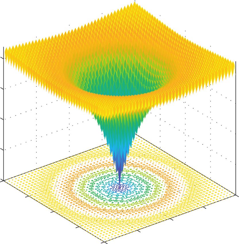
8 Computational Intelligence and Neuroscience

 Start

 Set parameters, initialize the location of
 the wolf pack

 Initialize SVM parameters, normalize
 training set

 Calculate the error score

 Run for the head wolf, update the position of
 the wolf pack

 Calculate the updated
 error score

 Run for the head wolf, update the position of
 wolf pack

 No Whether reach
 the maximum
 iterations ?

 Yes
 Optimal C,γ parameters

 Establish SVM model

 End

 Figure 8: Optimized flowchart.

 20

 15
 F10 ( x1, x2 )

 10

 5

 0
 20
 10 20
 0 10
 x2 0
 -10 -10 x1
 -20 -20

 Figure 9: Test function.
Computational Intelligence and Neuroscience 9

 100

 10-2

 10-4

 Best score
 10-6

 10-8

 10-10

 10-12

 10-14

 50 100 150 200 250 300 350 400 450 500
 Iteration
 GWO
 α-GWO
 Figure 10: Function optimization curve of GWO and α-GWO.

 0.15
 0.14
 0.13
 0.12
 Classification erro

 0.11
 0.1
 0.09
 0.08
 0.07
 0.06
 0.05
 0.04
 0 5 10 15 20 25 30
 Number of iterations

 α-GWO-SVM
 GWO-SVM
 Figure 11: Error curve of GWO-SVM and α-GWO-SVM.
10 Computational Intelligence and Neuroscience

 8

 7

 6

 Fault category labels
 5

 4

 3

 2

 1
 0 20 40 60 80 100
 Test set samples
 Actual category
 Diagnostic category
 Figure 12: Diagnosis results for the BFS of APSO-SVM.

 8

 7

 6
 Fault category labels

 5

 4

 3

 2

 1
 0 20 40 60 80 100
 Test set samples
 Actual category
 Diagnostic category
 Figure 13: Diagnosis results for the BFS of GWO-SVM.
Computational Intelligence and Neuroscience 11

 8

 7

 6

 Fault category labels
 5

 4

 3

 2

 1
 0 20 40 60 80 100
 Test set samples
 Actual category
 Diagnostic category
 Figure 14: Diagnosis results for the BFS of α-GWO-SVM.

 8

 7

 6
 Fault category labels

 5

 4

 3

 2

 1
 0 20 40 60 80 100
 Test set samples
 Actual category
 Diagnostic category
 Figure 15: Diagnosis results for the AFS of APSO-SVM.
12 Computational Intelligence and Neuroscience

 8

 7

 6

 Fault category labels
 5

 4

 3

 2

 1
 0 20 40 60 80 100
 Test set samples
 Actual category
 Diagnostic category
 Figure 16: Diagnosis results for the AFS of GWO-SVM.

 8

 7

 6
 Fault category labels

 5

 4

 3

 2

 1
 0 20 40 60 80 100
 Test set samples
 Actual category
 Diagnostic category
 Figure 17: Diagnosis results for the AFS of α-GWO-SVM.
Computational Intelligence and Neuroscience 13

 Table 2: Comparison of precision and kappa coefficient.
Diagnosis model APSO-SVM GWO-SVM α-GWO-SVM
Precision of the BFS 84.76% 92.51% 93.83%
Precision of the AFS 93.63% 94.47% 97.29%
Kappa coefficient of the BFS 84.30% 87.67% 89.91%
Kappa coefficient of the AFS 89.91% 91.03% 95.52%

 Table 3: Comparison of diagnosis results after feature fusion.
Diagnosis model APSO-SVM GWO-SVM α-GWO-SVM
Number of misclassification groups of the BFS 14 groups 11 groups 9 groups
Number of misclassification groups of the AFS 9 groups 8 groups 4 groups

 91

 81

 71

 61
 Precision (%)

 51

 41

 31

 21

 11

 1
 APSO-SVM GWO-SVM α-GWO-SVM

 BFS
 AFS
 Figure 18: Comparison of precision.

 91

 81

 71
 Kappa coefficient (%)

 61

 51

 41

 31

 21

 11

 1
 APSO-SVM GWO-SVM α-GWO-SVM

 BFS
 AFS
 Figure 19: Comparison of kappa coefficient.
14 Computational Intelligence and Neuroscience

are as few as 4 sets of samples getting misclassified. As References
compared to the BFS, the precision is improved by 2.82%
and kappa coefficient is increased by 4.49%, suggesting [1] X. L. Liu, Y. Zhao, W. J. Wang, and S. X. Ma, J. Zhuang, Photo
that the feature fusion is effective in enhancing the re- voltaic self-powered gas sensing: a review,” IEEE Sensors
 Journal, vol. 21, no. 5, pp. 5628–5644, 2021, https://ieeexplore.
liability of diagnosis.
 ieee.org/author/37088664419https://ieeexplore.ieee.org/
 author/37088663406.
5. Conclusion [2] T. Chen, Z. Saadatnia, J. Kim et al., “Novel, flexible, and
 ultrathin pressure feedback sensor for miniaturized intra-
The considerable contributions of the presented sensor fault ventricular neurosurgery robotic tools,” IEEE Transactions on
diagnosis method in comparison to the previous approaches Industrial Electronics, vol. 68, no. 5, pp. 4415–4425, 2021.
are summarized as follows: [3] P. Shan, H. Lv, L. Yu, H. Ge, Y. Li, and L. Gu, “A multisensor
 data fusion method for ball screw fault diagnosis based on
 (i) In order to improve the accuracy of sensor fault convolutional neural network with selected channels,” IEEE
 diagnosis, an integrated sensor fault diagnosis ap- Sensors Journal, vol. 20, no. 14, pp. 7896–7905, 2020.
 proach based on the combination of data-driven [4] M. Emperuman and S. Chandrasekaran, “Hybrid continuous
 and intelligent diagnosis is proposed in this paper. density hmm-based ensemble neural networks for sensor fault
 According to the results, this method is capable to detection and classification in wireless sensor network,”
 achieve an accurate diagnosis of sensor fault when Sensors, vol. 20, no. 3, p. 745, 2020.
 the failure intensity stays low. [5] D. Li, Y. Wang, J. Wang, C. Wang, and Y. Duan, “Recent
 advances in sensor fault diagnosis: a review,” Sensors and
 (ii In order to fully extract the valuable information
 Actuators A: Physical, vol. 309, Article ID 111990, 2020.
 from the fault data, a method of feature extraction is [6] D. Zhou, Y. Zhao, Z. Wang, X. He, and M. Gao, “Review on
 put forward based on the fusion of KPCA and time- diagnosis techniques for intermittent faults in dynamic sys-
 domain parameters, and experiments are conducted tems,” IEEE Transactions on Industrial Electronics, vol. 67,
 to demonstrate that the fusion feature improves the no. 3, pp. 2337–2347, 2020.
 accuracy of diagnosis effectively. [7] K. Choi, Y. Kim, S.-K. Kim, and K.-S. Kim, “Current and
 (iii) In addition, α-GWO algorithm is proposed to op- position sensor fault diagnosis algorithm for pmsm drives
 timize the parameters of SVM, thus enhancing the based on robust state observer,” IEEE Transactions on In-
 generalization ability of SVM. Through multiple dustrial Electronics, vol. 68, no. 6, pp. 5227–5236, 2021.
 [8] H. Shahnazari, “Fault diagnosis of nonlinear systems using
 comparison experiments and the analysis of per-
 recurrent neural networks,” Chemical Engineering Research
 formance indicators such as the precision and kappa and Design, vol. 153, pp. 233–245, 2020.
 coefficient, it is concluded that as compared to the [9] U. Saeed, S. U. Jan, Y. D. Lee, and I. Koo, “Fault diagnosis
 other intelligent diagnosis algorithms based on based on extremely randomized trees in wireless sensor
 SVM, the α-GWO-SVM diagnostic method pro- networks,” Reliability Engineering & System Safety, vol. 205,
 duces a better classification performance, and that Article ID 107284, 2021.
 the proposed method is effective in improving the [10] X. J. Luo and K. F. Fong, “Novel pattern recognition-en-
 reliability of diagnosis. In the future, the focus of hanced sensor fault detection and diagnosis for chiller plant,”
 research will be on the universality of this method Energy and Buildings, vol. 228, p. 110443, 2020.
 proposed. [11] N. Lu, H. Xiao, Y. Sun, M. Han, and Y. Wang, “A new method
 for intelligent fault diagnosis of machines based on unsu-
 pervised domain adaptation,” Neurocomputing, vol. 427,
Data Availability pp. 96–109, 2021.
 [12] Z. K. Song, L. C. Xu, X. Y. Hu, and Q. Li, “Research on fault
The data used to support the findings of this study are in- diagnosis method of axle box bearing of emu based on im-
cluded within the supplementary information file. proved shapelets algorithm,” Chinese Journal of Scientific
 Instrument, vol. 42, no. 2, pp. 66–74, 2021.
Conflicts of Interest [13] J. Wen, H. Yao, Z. Ji, B. Wu, and M. Xia, “On fault diagnosis
 for high-g accelerometers via data-driven models,” IEEE
The authors declare that they have no conflicts of interest. Sensors Journal, vol. 21, no. 2, pp. 1359–1368, 2021.
 [14] K. Jeong, S. B. Choi, and H. Choi, “Sensor fault detection and
 isolation using a support vector machine for vehicle sus-
Acknowledgments pension systems,” IEEE Transactions on Vehicular Technology,
This study was supported by the National Natural Science vol. 69, no. 4, pp. 3852–3863, 2020.
 [15] P. Yang, Z. Li, Z. Li, Y. Yu, J. Shi, and M. Sun, “Studies on fault
Foundation of China Program under grant no. 62073198 and
 diagnosis of dissolved oxygen sensor based on ga-svm,”
by the Major Research Development Program of Shandong
 Mathematical Biosciences and Engineering, vol. 18, no. 1,
Province of China under grant no. 2016GSF117009. pp. 386–399, 2021.
 [16] A. Soares, R. Râbelo, and A. Delbem, “Optimization based on
Supplementary Materials phylogram analysis,” Expert Systems with Applications,
 vol. 78, pp. 32–50, 2017.
“Experimental data.docx” contains the dataset used for the [17] R.-E. Precup, R.-C. David, R.-C. Roman, A.-I. Szedlak-Sti-
experiment in this paper. (Supplementary Materials) nean, and E. M. Petriu, “Optimal tuning of interval type-2
Computational Intelligence and Neuroscience 15

 fuzzy controllers for nonlinear servo systems using Slime
 Mould Algorithm,” International Journal of Systems Science,
 2021.
[18] B. H. Abed-Alguni, “Island-based cuckoo search with highly
 disruptive polynomial mutation,” International Journal of
 Artificial Intelligence, vol. 17, no. 1, pp. 57–82, 2019.
[19] H. Zapata, N. Perozo, W. Angulo, and J. Contreras, “A Hybrid
 Swarm algorithm for collective construction of 3D struc-
 tures,” International Journal of Artificial Intelligence, vol. 18,
 no. 1, pp. 1–18, 2020.
[20] R.-E. Precup, E.-L. Hedrea, R.-C. Roman, E. M. Petriu,
 A.-I. Szedlak-Stinean, and C.-A. Bojan-Dragos, “Experiment-
 based approach to teach optimization techniques,” IEEE
 Transactions on Education, vol. 64, no. 2, pp. 88–94, 2021.
[21] H. Lahdhiri and O. Taouali, “Interval valued data driven
 approach for sensor fault detection of nonlinear uncertain
 process,” Measurement, vol. 171, Article ID 108776, 2021.
[22] J. G. Qian, “Diagnosis of machinery fault by time-domain
 parameters,” Coal Mine Machinery, vol. 27, no. 09,
 pp. 192-193, 2006.
[23] S. Mirjalili, S. M. Mirjalili, and A. Lewis, “Grey wolf opti-
 mizer,” Advances in Engineering Software, vol. 69, pp. 46–61,
 2014.
[24] J. H. Yang, F. J. Xiong, D. Q. Wu, D. S. Xie, and J. M. Yang,
 “Maximum power point tracking of wave power system based
 on fourier analysis method and modified grey wolf opti-
 mizer,” Acta Energiae Solaris Sinica, vol. 42, no. 1, pp. 406–
 415, 2021.
[25] X. F. Yuan, Z. H. Yan, F. Y. Zhou, Y. Song, and Z. M. Miao,
 “Rolling bearing fault diadnosis based on stacked sparse auto-
 encoding network and igwo-svm,” Journal of Vibration,
 Measurement & Diagnosis, vol. 40, no. 2, pp. 405–413+424,
 2021.
[26] Intel lab data. Available online: https://db.csail.mit.edu/
 labdata/labdata.html.. (accessed on 13 June 2019.
[27] B. D. Bruijn, T. A. Nguyen, D. Bucur, and K. Tei, “Benchmark
 datasets for fault detection and classification in sensor data,”
 in Proceedings of the 5th International Conference on Sensor
 Networks, pp. 185–195, Rome, Italy, February 2016.
[28] Y. C. Li, R. X. Qiu, and J. Zeng, “Blind online false data
 injection attack using kernel principal component analysis in
 smart grid,” Power System Technology, vol. 42, no. 7,
 pp. 2270–2278, 2018.
[29] C. Cortes and V. Vapnik, “Support-vector networks,” Ma-
 chine Learning, vol. 20, no. 3, pp. 273–297, 1995.
[30] Y. Wang, G. Q. Liang, and Y. T. Wei, “Road identification
 algorithm of intelligent tire based on support vector ma-
 chine,” Automotive Engineering, vol. 42, no. 12,
 pp. 1671–1678+1717, 2020.
[31] C.-F. Chao and M.-H. Horng, “The construction of support
 vector machine classifier using the firefly algorithm,” Com-
 putational Intelligence and Neuroscience, vol. 2015, pp. 1–8,
 2015.
[32] J. Zhang, Z. B. Liu, W. R. Song, L. Z. Fu, and Y. l. Zhang,
 “Stellar spectra classification method based on multi-class
 support vector machine,” Spectroscopy and Spectral Analysis,
 vol. 38, no. 7, pp. 2307–2310, 2018.
[33] Z. L Tan and X. C. Chen, “Study on improved classifiers’s
 performance evaluation indicators,” Statistic &. Information
 Forum, vol. 35, no. 9, pp. 3–8, 2020.
[34] S. Das, H. Mukherjee, K. Roy, and C. K. Saha, “Shortcoming of
 visual interpretation of cardiotocography: a comparative study
 with automated method and established guideline using statistical
 analysis,” SN Computer Science, vol. 1, no. 3, pp. 180–190, 2020.
You can also read


