A No-Regret Framework For Deriving Optimal Strategies With Emphasis On Trading In Electronic Markets - Princeton University
←
→
Page content transcription
If your browser does not render page correctly, please read the page content below
A No-Regret Framework For Deriving
Optimal Strategies With Emphasis On
   Trading In Electronic Markets

              Pranjit Kumar Kalita

                A Master’s Thesis
             Presented to the Faculty
             of Princeton University
           in Candidacy for the Degree
        of Master of Science in Engineering

           Recommended for Acceptance
               by the Department of
                Computer Science
      Adviser: Professor S. Matthew Weinberg

                    June 2018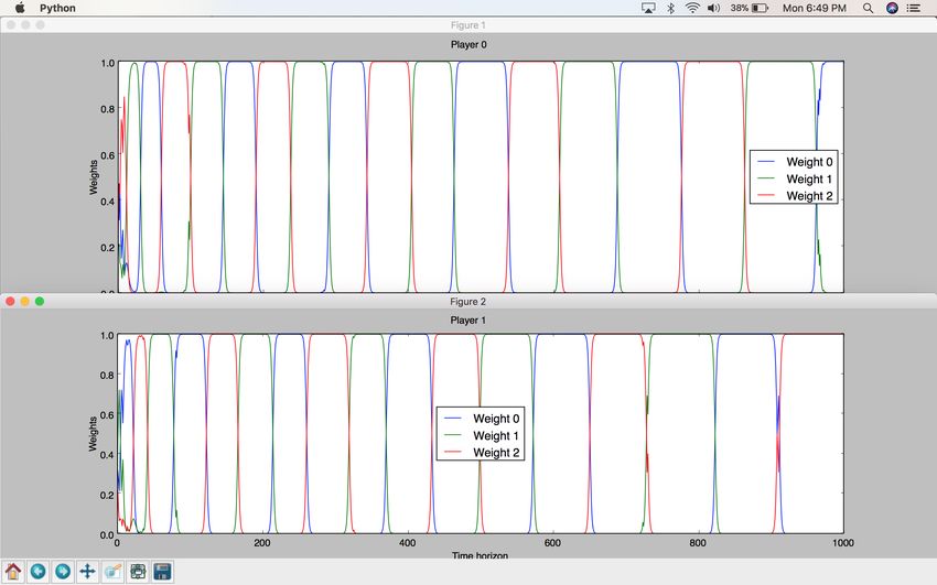
c Copyright by Pranjit Kumar Kalita, 2018.

           All rights reserved.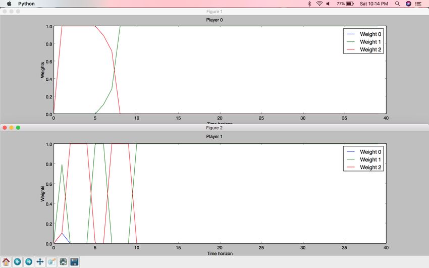
Abstract

We present a no-regret learning framework to analyze behavior of strategic agents
within single and multi-player games. We introduce a tool that could be used for
any game to calculate optimal strategies for each player. Specifically, we base our
tool on two regret minimization algorithms - Multiplicative Weights [5] and EXP3 [6].

We begin by describing each of the two regret minimization algorithms used
followed by justification of our system design. Then, for proof of concept, we test
our tool on two known games. Then, given that the main intention of this work is to
measure the viability of applying a regret minimization framework within a trading
environment, we move our discussion to describing our market framework followed
by testing on an abstract trading game. That trading game is one that is designed
based on certain abstractions, which will be described in detail. We then evaluate the
application of our framework for that trading game with future potential of applying
to further trading environments.

A significant amount of effort was dedicated towards understanding the market
microstructure of an electronic market order book system.        We will describe in
detail our implementation of a zero-intelligence [3] market environment, and the
implications and results for using the same. The trading game developed and tested
is inherently linked to this market environment and the randomness of the market
was instrumental in designing the game used.

                                          iii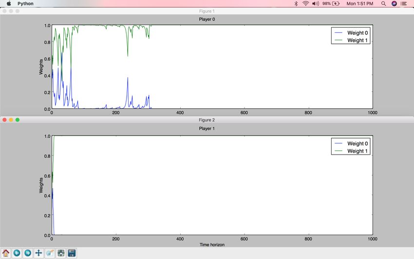
Acknowledgements

I would like to extend a debt of gratitude to my thesis advisor Professor S. Matthew
Weinberg, Assistant Professor, Department of Computer Science, Princeton Univer-
sity, for guiding my thesis. He has been very instrumental in helping me understand
the intuition and theory behind regret-minimization and game theory, and has been
very keen in learning and informing me about the financial markets and trading,
which were unfamiliar territories for him.

I would further like to thank Dr.      Robert Almgren, Adjunct Professor in the
Department of Operations Research and Financial Engineering, for his patience in
explaining to me the dynamics of the electronic market microstructure and suggest-
ing to me the paper on zero-intelligence, which formed the backbone of our market
environment. He did not have any official affiliation with me or my project, so his
generosity in this regard, especially during a time when I was lost while designing a
market environment without accounting for market impact to execute trades on, will
never be forgotten.

Finally, I would like to thank Dr.       Han Liu, formerly Assistant Professor of
Operations Research and Financial Engineering, who introduced me to the world of
systematic and quantitative trading using Python and guided my development in
the field of finance and trading through an online course he suggested me to take to
ultimately expand my horizons in this project's most critical intended impact area.

                                         iv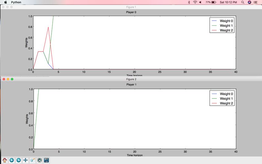
Contents

Abstract                                                                              iii

Acknowledgements                                                                      iv

1 Introduction                                                                         1

2 Background                                                                           3
  2.1   The Regret-Minimization Problem . . . . . . . . . . . . . . . . . . . .        3
  2.2   The Multiplicative Weights Algorithm . . . . . . . . . . . . . . . . .         4
  2.3   The EXP3 Algorithm . . . . . . . . . . . . . . . . . . . . . . . . . . .       5
  2.4   The Zero-Intelligence Market Model [3] . . . . . . . . . . . . . . . . .       7
        2.4.1   Continuous Double Auction [3] . . . . . . . . . . . . . . . . .        8
        2.4.2   Review of the Model [3] . . . . . . . . . . . . . . . . . . . . .      9
        2.4.3   Assumptions of the model . . . . . . . . . . . . . . . . . . . .       9
  2.5   Architectural Considerations while designing the tool . . . . . . . . .       10

3 Our No-Regret Framework                                                             12
  3.1   Structure of the Input File . . . . . . . . . . . . . . . . . . . . . . . .   12
  3.2   Objects Used to Store Information . . . . . . . . . . . . . . . . . . .       13
  3.3   Framework for playing the game . . . . . . . . . . . . . . . . . . . . .      14

4 Our implementation of the Zero-Intelligence Market                                  16
  4.1   The Zero-Intelligence Market . . . . . . . . . . . . . . . . . . . . . . .    18
        4.1.1   Initializing the Market . . . . . . . . . . . . . . . . . . . . . .   18
        4.1.2   Creating the rest of the market processes . . . . . . . . . . . .     19

5 Results                                                                             22
  5.1   Rock-Paper-Scissors . . . . . . . . . . . . . . . . . . . . . . . . . . . .   22
        5.1.1   Multiplicative Weights . . . . . . . . . . . . . . . . . . . . . .    22
                                           v
5.1.2   EXP3 . . . . . . . . . . . . . . . . . . . . . . . . . . . . . . .   23
  5.2   Prisoner’s Dilemma . . . . . . . . . . . . . . . . . . . . . . . . . . . .   24
        5.2.1   Multiplicative Weights . . . . . . . . . . . . . . . . . . . . . .   25
        5.2.2   EXP3 . . . . . . . . . . . . . . . . . . . . . . . . . . . . . . .   26
  5.3   Abstract Two Spoofer game . . . . . . . . . . . . . . . . . . . . . . .      27
        5.3.1   Multiplicative Weights . . . . . . . . . . . . . . . . . . . . . .   29
        5.3.2   EXP3 . . . . . . . . . . . . . . . . . . . . . . . . . . . . . . .   32

6 Conclusion                                                                         34

7 Future Work                                                                        35

References                                                                           37

                                          vi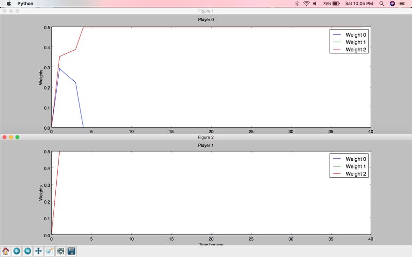
1    Introduction

In this paper, we discuss the implementation of a no-regret learning framework to
games. The games could be single player and multi-player, with specific payoff-
s/rewards. Emphasis is placed on the background of two no-regret algorithms -
Multiplicative Weights and EXP3, as well as the design of the tool that incorporates
these learning algorithms within a game theoretic setting. We describe in detail
our architectural decisions behind the tool. The evaluation of our tool is done on
two known games to calculate optimal strategies of two players playing the game -
Rock-Paper-Scissors and Prisoner’s Dilemma. We show that our framework yields
the expected cyclical behavior of strategies on the first game, and the correct Nash
Equilibrium for the second [1]. This step is essential to ensure the correctness of our
framework to any known game.

With the intention of applying no-regret learning within the context of trading,
we then discuss our implementation of a market model, based on electronic limit
order books. We use the zero-intelligence market model primarily to account for the
problem of measuring market impact of traders’ actions within the market. After
ascertaining the correctness of our market model, we then construct an abstract
trading game based on a few assumptions, and try to construct a game out of a
general type of market manipulation algorithms known as spoofing [4]. In short,
spoofing is a means of manipulating markets by executing a fake order to generate
market behavior which a trader correctly foresees and benefits from. With certain
abstractions of the market place, we created a game and analyzed the behavior of
traders under a situation when there are two active spoofers.

We were inspired to create this project from scratch because of our shared in-
terests in game theory and understanding human behavior in dynamic environments.
                                          1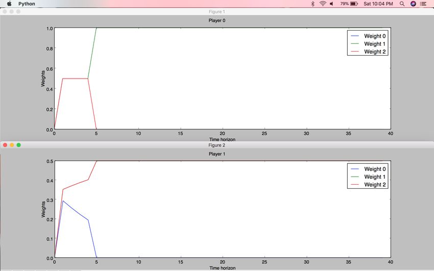
The markets are perhaps the most dynamic environment there is and we wanted
to build a tool that could help traders strategize their activities, to bring in new
rationality to their behaviors, especially when known events and market forces are
seen again.

                                         2
2     Background

In this section we will discuss concepts and work related to this project. We will first
describe what we mean by no-regret learning and the regret-minimization problem.
Then, we will give an overview of Multiplicative Weights and EXP3 algorithms and
explain the reasons for selecting these algorithms within our framework. We will then
discuss the zero-intelligence market model, and why it is desirable for the purposes
of our project. Finally, we give an overview of our architectural considerations while
designing the tool.

2.1      The Regret-Minimization Problem

An attractive feature of no-regret dynamics in multi-player games is their rapid
convergence to an approximate equilibrium [5]. Let us begin by looking at the
regret-minimization problem, which studies a single decision-maker playing a game
against an adversary. Then we will connect the single-player setting to multi-player
games.

The following is the setup for a set of actions A. The number of actions n ≥ 2. [5]

    • At time t = 1, 2, ..., T :

         – A decision maker picks a mixed strategy pt - that is, a probability distri-
            bution over its actions A.

         – An adversary picks a cost vector ct : A− > [0, 1]1 .

         – An action at is chosen according to the distribution pt , and the decision
            maker incurs cost ct (at ). The decision maker learns the entire cost vector
            ct , not just the realized cost ct (at ).

                                                3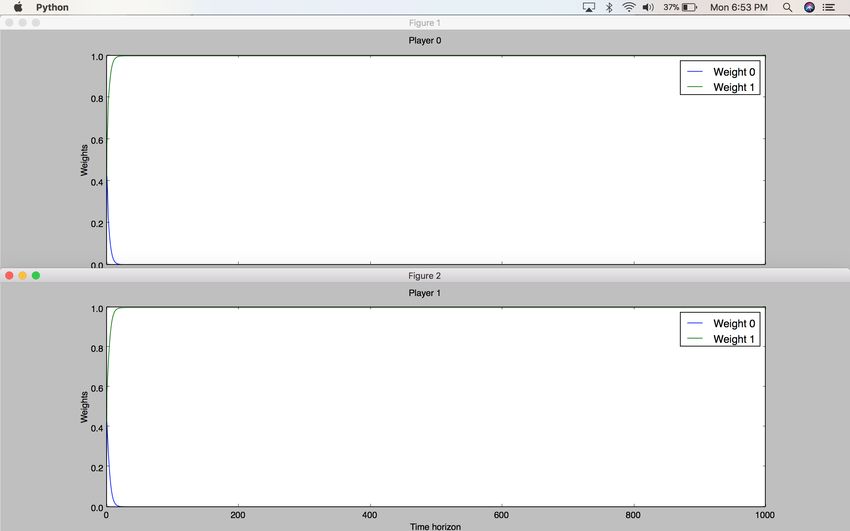
Definition 2.1.1 (Regret)            The time-averaged regret of the action sequence
                                               1 PT                   PT
a1 , ..., aT with respect to the action a is   T
                                                 [ t=1 ct (at )   −    i=1   ct (a)]. [5]

Definition 2.1.2 (No-Regret Algorithm) Let α be an online decision-making
problem.

      1. An adversary for α is a function that takes as input the time t, the mixed
         strategies p1 , ..., pt produced by α on the first t times, and the realized actions
         a1 , ..., at−1 of the time (t − 1) times, and produces as output a cost vector
         ct : [0, 1]− > A.

      2. An online decision-making algorithm has no regret if for every adversary for it,
         the expected regret with respect to every action a ∈ A is o(1) as T − > ∞. [5]

Result 2.1.1 (Regret Lower Bound) With n actions, no algorithm has expected
                                    q
regret vanishing faster than Θ( (ln n)/T . [5]

2.2       The Multiplicative Weights Algorithm

The design of Multiplicative Weights algorithm has the following design principles:
[5]

      1. Past performance of actions should guide which action is chosen now.

      2. Many instantiations of the above idea yield no-regret algorithms. For optimal
         regret bounds however, it is important to aggressively punish bad actions - when
         a previously good action turns sour, the probability with which it is played
         should decrease at an exponential rate.

The formal description of the algorithm is as follows: [5]

      1. Initialize w1 (a) = 1 for every a ∈ A.
                                                4
2. For t = 1, 2, ..., T :
(a) Play an action according to the distribution pt = wt /τ t , where τ t =
wt (a) is the sum of the weights.
P
a∈A
(b) Given the cost vector ct , decrease weights using the formula wt+1 (a) =
t
wt (a) ∗ (1 − )(c (a)) for every action a ∈ A.
is the learning rate, which will be between 0 and 12 .
The fundamental reason for using Multiplicative Weights as our no-regret learn-
q
ing algorithm is that the (per-time-step) regret is at most 2 (ln n)/T [5], which
is the regret lower bound result from Result 2.1.1. The learning rate parameter
q
is chosen as = (ln n)/T , which achieves the regret lower bound on the algorithm.
q
Remark 2.2.1 (When T is Unknown) = (ln n)/T̂ , where T̂ is the smallest
power of 2 greater than or equal to t.
Now we will extend Multiplicative Weights from single-player to multi-player
settings. In each time step t = 1, 2, ..., T of no-regret learning in a multi-player
setting (no-regret dynamics):
1. Each player i simultaneously and independently chooses a mixed strategy pti
using a no-regret algorithm.
2. Each player i receives a cost vector cti , where cti (si ) is the expected cost of
strategy si when the other players play their chosen mixed strategies.
2.3 The EXP3 Algorithm
The EXP3 Algorithm works within the MultiArmed Bandit (MAB) problem frame-
work. In this model, there is a set of N actions from which the player has to choose
5in every time step t ∈ T . After that action is chosen, the player can see the loss
of that action, but not of that of the other possible actions. An example of the
MAB problem includes choosing a route to take to work, where the driver does not
know the losses of routes outside of the route that they end up taking. The EXP3
Algorithm is one of the regret minimization algorithms within the category of MAB
problems.
The general idea of the EXP3 algorithm is the following: [6]
• At time t, the player chooses actions according to the distribution pt - i.e.,
choose action i with probability pt (i).
• The player receives a profit for action i of gt (i). (In EXP3, the objective is to
maximize profits instead of minimizing losses.)
gt (i)
• The player updates the estimate for the sum of profits of action i by pt (i)
.
P gt (i)
The expectation of the profit of i is roughly the sum: E[estimate of i’s profit]= t pt (i)
The EXP3 algorithm is based on the exponential weights regret minimization
algorithm. We have a learning parameter η ∈ [0, 1]. Each action is originally
assigned a weight wi = 1, i.e., ∀i ∈ [1, 2, ..., N ], wi = 1. Wt is defined as the sum of
PN
the weights of the actions at time t: Wt = i=1 wi (t). Then, Wt is used to normalize
the probabilities pi of actions. [6]
At time t, [6]
1. pi (t) = (1 − η) wWi (t)
t
+ η N1 , i.e., pi (t) is proportional to the relative weight of i
with a small correction to ensure that pi is never too close to 0.
2. Player chooses an action it (a random variable) according to the distribution
p1 (t), ..., pN (t).
63. The player receives a profit gi (t) ∈ [0, 1].
4. Define ĝ j (t) = { gj (t)pj (t), if j = it
0, otherwise
5. Update the weights of the actions: wj (t + 1) = wj (t)eηĝj (t)/N
In short, the weights give an estimate of how good the actions are. Actions get
chosen with probability relative to their weights, and the weights are updated in an
exponential fashion.
Remark 2.2.1 (Regret Bound of the EXP3 Algorithm) EXP3 reaches
√
a regret bound of O T by combining the exploration and exploitation stages of the
MAB algorithm. [6]
2.4 The Zero-Intelligence Market Model [3]
A significant amount of time was devoted to finding the right market model to test
our no-regret learning framework on within the context of trading activities. The
most significant issue faced was the question of how to account for market impact of
executed strategies. This quest to understand a market model which would allow us
to operate under conditions of predictable market impact of our trades, or at least
one that would allow us to not assume our cost of market activities, led to adapting
the zero-intelligence model, also known as the Santa-Fe Model. The model also does
a good job of predicting the average spread, and the price diffusion rate. [3]
The main components of the zero-intelligence market model will be described
in the sections below.
72.4.1 Continuous Double Auction [3]
The zero-intelligence market assumes a continuous double auction, the most widely
used method of price formation in modern electronic markets. The orders are catego-
rized into two types: market orders, which are requests to buy or sell a desired number
of shares immediately at the best available price, i.e., the market quote. Limit orders
are the other type of orders which specify a limit below (or above) which a sell (or
buy) order will not execute. Limit orders may not result in an immediate transaction,
in which case are stored in a queue called the limit order book (see Figure 1). As each
buy order arrives it is transacted against accumulated sell limit orders that have a
lower selling price, in priority of price and arrival time, and vice-versa for sell orders.
The best ask, a(t) is the lowest selling price offered in the book at any point in time.
The best bid, b(t) is the highest buying price offered in the book at any point in time.
Figure 1: A random process model of the continuous double auction. Stored limit
orders are shown stacked along the price axis, with sell orders (supply) stacked above
the axis at higher prices and buy prices (demand) stacked below the axis at lower
prices. New sell limit orders are visualized as randomly falling down, and new buy
orders as randomly falling up. New sell orders can be placed anywhere above the
best buying price, and new buy orders anywhere below the best selling price. Limit
orders can be removed spontaneously (e.g. because the agent changes their mind or
the order expires) or they can be removed by market orders of the opposite type.
This can result in changes in the best prices, which in turn alters the boundaries of
the order placement process. It is this feedback between order placement and price
formation that makes this model interesting, and its predictions non-trivial. [3]
82.4.2 Review of the Model [3]
The model calls market order placing agents as impatient agents, and limit order
placing agents as patient agents. It assumes that they are zero intelligence agents
that place and cancel orders randomly, as shown in Figure 1. Impatient agents place
market orders of size σ, which arrive at a rate µ shares per time. Patient agents plae
limit orders of the size σ, which arrive with a constant rate density α shares per price
per time. Queued limit orders are canceled at a constant rate δ, with dimensions of
1/time. Prices change in discrete increments called ticks, of size dp. The rates of
buying and selling are considered to be equal, and limit/market order placement and
cancellation processes are Poisson processes. All of these processes are independent
except for coupling through their boundary conditions: Buy limit orders arrive with
a constant density α over the interval −∞ < p < a(t), where p is the logarithm
of the price; and sell limit orders arrive with a constant density α over the interval
b(t) < p < ∞. As a result of the random order arrival processes, a(t) and b(t) each
make random walks, but because of coupling of the buying and selling processes the
bid-ask spread s(t) = a(t) - b(t) is a stationary random variable.
New orders may alter the best prices a(t) and b(t), which in turn changes the
boundary conditions for subsequent limit order placement. For example, the arrival
of a limit buy order inside the spread will alter the best bid b(t), which then alters
the boundary condition for sell limit order placement, and vice-versa. This feedback
between order placement and price diffusion makes this model interesting.
2.4.3 Assumptions of the model
The model makes some strong assumptions.
• It assumes that the rates for buying and selling are equal.
9• The sizes of limit and market orders are the same.
• Limit order deposition is uniform on semi-infinite intervals.
• Rates of order submissions are unaffected by price changes.
The only participants in this market are zero-intelligence noise traders that randomly
supply and demand liquidity. This model is intended to be used as primarily to
provide a background market to execute trades on, where the question of market
impact is readily answered and without assumptions.
2.5 Architectural Considerations while designing the tool
Our main tool consists of the framework that allows single- and multi-player games
to be played and analyzed. The main design choices implemented -
• Automatic input of the game participants, its number, strategies available per
participant, and payoff matrix through files.
• Ability to spawn multiple threads per round wherein each player could inde-
pendently implement their next action.
Our implementation of the zero-intelligence market model makes the following design
and architectural considerations and assumptions -
• Prices were assumed to be in absolute units and not logarithmic.
• Order size of market and limit orders (σ) were assumed to be unit sized.
• Tick size of 1 price unit was used.
• 5 units of price from the best market price of both ask and bid were used to place
the minimum and maximum range of bids and sells, respectively. For example:
if the lowest ask a(t) = 104, then bids (t) could be in the range 98 < b(t) < 104,
¯
10spaced by tick size. Similarly, if the highest bid b(t) = 102, then asks t) could
be in the range 102 < a(t) < 108, spaced by tick size.
• Extensive use of multi-threaded programming and multi-programming while
executing the zero-intelligence market model.
113 Our No-Regret Framework
In this section, we describe our tool for finding optimal strategies in single- and
multi-player games, followed by an in-depth look at our design of the zero-intelligence
market model. We also describe the nature of input to our tool.
The development of the tool took place in stages. We started off by creating a
manual-input version for deciding payoffs/costs per strategy while playing a game,
eventually moving on to file input where information about the payoff/cost matrix,
number of players and number of strategies per player is pre-written. Here, we will
only describe our finished tool where multiple players execute their strategies and
update actions’ weight matrices per time step in independent threads, with input
being fed from files.
The framework is the same for both Multiplicative Weights and the EXP3 al-
gorithms, with the underlying changes only being with respect to the learning
parameters used ( and η, respectively) and the means with which the players’
weights for strategies are changed for the next round. Finally, in order to visualize
which strategies are winning out, for each player, at each time step, we normalize
weights for each strategy.
3.1 Structure of the Input File
Each game has a corresponding input file that stores the following information:
• Number of strategies per player (N ) - at the beginning of the game, this gets
read into a variable.
• Number of players (N umP l) - at the beginning of the game, this gets read into
a variable.
12• Cost(Payoff) Matrix describing what the cost(payoff) would be for Multiplica-
tive Weights(EXP3) per player per strategy depending on what the other play-
ers’ strategies are. It is of dimensions (N N umP l x N umP l). This gets stored into
a multi-dimensional cost(payoff) array during the initialization of the game.
3.2 Objects Used to Store Information
We employ the following classes to store information about and execute the game -
1. Environment Class - the environment that runs the game. Has the following
data variables and member function -
(a) Number of strategies per player (N )
(b) Number of players (N umP l)
(c) Cost(Payoff) Matrix in a multi-dimensional array
(d) generateRewards() function - this function will, based on strategies of all
players during tth round, return an array of cost(payoff) values per player.
2. Player Class - used to store each players’ strategies and how they are perform-
ing. Has the following data variables and member functions -
(a) Total time for which the game will be played (T ).
(b) Number of strategies (N ).
(c) Weight Matrix for actions (wN ×T )
(d) Normalized Weight Matrix for actions (WN ×T )
(e) (Only for EXP3) A Probability array of size (1 × N ) proportional to the
relative weight of each strategy.
(f) Learning parameter ( and η corresponding to Multiplicative Weights and
q q
EXP3, respectively). = ln N/T and η = 10 ∗ (N ∗ ln N )/(2 ∗ T ). The
13choice of and η are picked based on no-regret bound theorems described
in Result 2.1.1 and Theorem 4.1 of [6]. The factor 10 is added to η to
make the weight plots more prominent, and serves no theoretical purpose.
(g) pickStrategy() function - picks a strategy according to the probability dis-
tribution discretized over weights of individual actions. (For EXP3, di-
rectly use the probability array belonging to the player. For Mul-
tiplicative Weights, generate the probability distribution over the
individual weights within function.)
(h) changeWeight() function - Change weights of strategies for the (t + 1)th
step depending on the cost(payoff) incurred during the tth step. (Note
that Multiplicative Weights and EXP3 differ in exploration vs.
exploitation [6] in that the former updates the weights of all
strategies not taken per the strategies taken by the other play-
ers, whereas the latter only updates weight for the strategy taken
in the previous step. Multiplicative Weights is an example of ex-
ploration; EXP3 is an example of exploitation.) Finally, normalize
the weights in this function so as to visualize the effect of playing the game
over time on deriving winning/optimal strategies.
3.3 Framework for playing the game
• Initialize the environment and player objects based on input from the file storing
game structure, and time over which to analyze strategies (provided manually).
• At each time step t -
1. Spawn N umP l number of threads, each for a player to pick their strategy
for time step t (call pickStrategy() function for each player).
142. Wait for all threads to join, at which point generate the rewards (call
generateRewards() function of environment) for each player based on the
actions chosen. It is important for threads to join before changing weights
for two reasons -
(a) Time step for each player remains the same, i.e., all players move from
time t to t + 1 only after they have all finished picking strategies.
(b) Multiplicative Weights needs to know the information for strategies
picked by other players in order to set weights of actions not taken at
time step t (exploration [6]).
3. Spawn another set of N umP l threads, each for a player to change weights
of their actions (call changeWeights() function for each player).
4. Wait for all threads to join, then move to the next time step.
• When T time steps have been played for each player, then finish the game
and show the results of players’ game theoretic behavior through plotting the
normalized plots for their individual weight strategies per time step.
A snapshot of execution of the game is presented in Figure 2 below.
Figure 2: Behavior of our tool as players pick and execute strategies from time step
0 to time step 1. Note the messages in red show multi-threaded programming in
action; The vectors shown are weight matrices of Player0 and Player1 (there is a time
lag to standard output due to different thread executions simultaneously hence the
misplacement of messages with respect to the weight vectors on the main method).
154 Our implementation of the Zero-Intelligence
Market
We employ the following classes to interface directly with the market -
1. Limit Order Book Class - the limit order book of the market. Consists of the
following data members and member functions -
(a) Limit Buys - Will store the limit buy order queue. Limit buys are 3-
dimensional vectors of (price, time, order id). They will be arranged in
decreasing order of price and increasing order of time, i.e., the highest bid
offer at the earliest time will be put in front of the queue.
(b) Limit Sells - Will store the limit sell order queue. Limit sells are 3-
dimensional vectors of (price, time, order id). They will be arranged in
increasing order of price and increasing order of time, i.e., the lowest sell
offer at the earliest time will be put in front of the queue.
(c) Limit Buy Count - to keep count of the number of outstanding limit buy
offers that have not yet expired.
(d) Limit Sell Count - to keep count of the number of outstanding limit sell
offers that have not yet expired.
(e) addLimitOrder() - a function to add a new limit order to the limit order
book.
(f) delLimitBuy() - a function that matches a market sell order with the limit
buy atop the limit buys queue and deletes the limit buy count by 1.
(g) delLimitSell() - a function that matches a market buy order with the limit
sell atop the limit sells queue and deletes the limit sell count by 1.
(h) getHighestBid() - returns the highest and earliest bid at any point in time.
16(i) getLowestAsk() - returns the lowest and earliest ask at any point in time.
(j) showLOB() - show the contents of the limit order book.
2. Limit Order Class - the limit order generated by each market participant.
Consists of the following data members and member functions -
(a) id - to store the order identity (distinguish between orders).
(b) buyOrSell - indicate whether it is a buy or sell order by an indicator vari-
able passed to each Limit Order class object.
(c) price - the price for bid or ask.
(d) timeBegan - when the order originated.
(e) cancellationTime - for how long will the order stay.
(f) orderSize - the size of the order (constant σ used).
(g) endTime - timeBegan + cancellationT ime. Indicates when the limit order
expires.
(h) lob - the Limit Order Book object where limit orders are being submitted
and stored.
(i) showCharacteristics() - a function to show the characteristics of the limit
order.
(j) poke() - a function that spawns a background thread per limit order that
keeps poking the limit order book ’lob’ to check whether or not the limit
order has expired. If it has, it removes the corresponding order from the
limit order book.
3. Trader Class - to generate limit orders based on trading strategies. This is a
basic class in which the trader will, based on the limit order book information,
implement a trading strategy and generate a limit order on the buy or sell side.
Its data members and member functions include -
17(a) lob - the Limit Order Book object where limit orders are being submitted
and stored.
(b) generateLimitOrder() - function to generate a limt order based on specific
trading strategies informed by the limit order book.
Note: The Trader class handles simple trading strategies and interfaces di-
rectly with the market; however due to being unable to account for calculating
proper cost(reward) functions within the zero-intelligence framework, it is be-
ing kept open for future extension as well as use within our larger no-regret
framework.
4.1 The Zero-Intelligence Market
Definition 4.1.1 A Poisson process is F (t) = 1 − e−λt , where t is the elapsed time
and F (t) is the probability that the poisson process will happen t time units into the
future. λ is the rate parameter of the Poisson process.
Definition 4.1.2 If a process follows the Poisson process, then the time for the
next event is : t = − ln(1 − F (t))/λ, F (t) ∈ [0.0, 1.0), λ is the rate parameter.
Limit buy orders, limit sell orders, market buy orders and market sell orders each
have their own Poisson process for generating orders, which means they have their
own rate parameter λ. Similarly, the order cancellation rate for each limit order is a
separate Poisson process with its own rate parameter λ.
4.1.1 Initializing the Market
First, select values for lowest ask and highest bid, and the rate parameters for Poisson
processes. Initially fill in the limit order book before taking in market orders. In order
to do this, for a certain period of time, say 20 seconds, we do the following in a loop:
181. Create multiple processes to find the next time that a limit buy and limit sell
is generated, using their respective λ’s and using Definition 4.1.2.
2. Wait for both processes to join.
3. Pick the earliest between the two.
4. Now, since limit orders are poisson processes over (price x time), once the time
is picked, it is time to pick a price. We select a range of prices to be picked
uniformly over a discrete distribution described in Section 2.5.
5. Add the picked process to the limit order book.
At this point the limit order book is filled (Figure 3).
4.1.2 Creating the rest of the market processes
Once the market has been initialized, it is time to generate the rest of the zero-
intelligence market activity. Do the following in an infinite loop:
1. Create multiple processes to find the next time that a limit buy, limit sell,
market buy and market sell is generated, using their respective λ’s and using
Definition 4.1.2.
2. Wait for all 4 processes to join.
3. Pick the earliest among the 4, and then spawn another thread to create the
next market or limit order based on the picked process to be generated next.
That thread has to join in before the next iteration of the loop continues.
(a) If it is a market sell that was picked, then simply delete the first entry
within the limit buy queue (Figure 4).
(b) If it is a market buy that was picked, then simply delete the first entry
within the limit sell queue (Figure 5).
19(c) If it is a limit sell that was picked, then if matched with a limit buy,
delete the first entries of both limit buy and limit sell queues (Figure 6).
Vice-versa for limit buy.
(d) If a limit sell or limit buy wasn’t matched, then add to the appropriate
position within the corresponding queue in the limit order book (Figure
7). In this case, we also spawn a thread to begin the poke() process of
the limit order (sell or buy). This process will run in the background until
either the limit order gets matched with a market or limit order of the
opposite direction, or reaches its expiration time (the order cancellation
rate is used to calculate the cancellation time for a limit order). Note:
The price picking process for limit orders is similar to the one described
for limit orders during the initialization phase in Section 4.1.1.
We also have a separate thread running in the background that pokes prospec-
tive traders (each with their own trading strategies) for their orders. We
have provided the framework for traders to execute their trading strategies
within this zero-intelligence market once questions about calculating the right
rewards(payoffs) per trading strategy are answered. For the time-being, we only
describe a fully-functioning zero-intelligence market.
The figures following (3-7) show various functions during execution of the zero-
intelligence market.
Figure 3: Initializing the zero-intelligence market with limit orders.
20Figure 4: Market sell order generated and it simply removes the first element in limit
buy queue. The highest bid, lowest ask, and spread values are then updated.
Figure 5: Market buy order generated and it simply removes the first element in limit
sell queue. The highest bid, lowest ask, and spread values are then updated.
Figure 6: Showing Matching of limit buy with limit sell, and updating of the highest
bid, lowest ask values.
Figure 7: A limit order was generated but it was pushed down in the limit order book
queue and no trading took place.
215 Results
5.1 Rock-Paper-Scissors
Rock-Paper-Scissors is a popular hand-game that is played between two players, each
having three strategies - Rock, Paper and Scissors. The structure of the game is -
• Paper beats Rock
• Scissors beats Paper
• Rock beats Scissors
Accordingly, we set our game and payoff matrix and run our two no-regret learning
algorithms to find optimal strategies in both players.
In our simulation, we set -
• Strategy0 to be Rock
• Strategy1 to be Paper
• Strategy2 to be Scissors
5.1.1 Multiplicative Weights
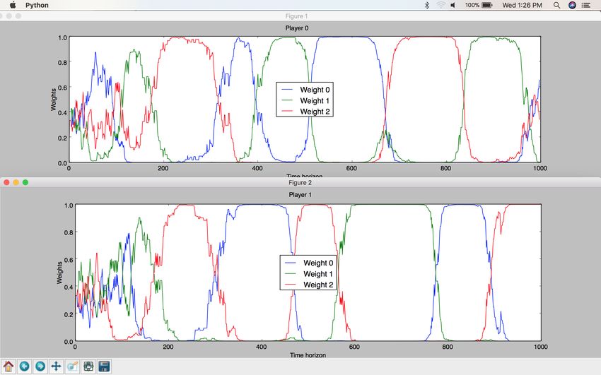
22Figure 8: Multiplicative Weights Algorithm results on Rock-Paper-Scissors game.
Weight 0 corresponds to the weight of Strategy0, Weight 1 corresponds to the
weight of Strategy1, Weight 2 corresponds to the weight of Strategy2.
We note that both players exhibit a cyclical behavior in their strategies picked over
time. As one player is strong on Scissors, the other player begins to realize that the
winning strategy is to pick Rock. As the latter’s Rock strategy begins to win more
often, the first player begins to realize that Paper could beat the opposing player’s
Rock. Scissors then beats Paper, and this cycle repeats itself until the end of the
simulation, leading to an optimal game strategy for Rock-Paper-Scissors.
5.1.2 EXP3
23Figure 9: EXP3 Algorithm results on Rock-Paper-Scissors game. Weight 0 corre-
sponds to the weight of Strategy0, Weight 1 corresponds to the weight of Strategy1,
Weight 2 corresponds to the weight of Strategy2.
We note that both players exhibit a cyclical behavior in their strategies picked over
time. As one player is strong on Scissors, the other player begins to realize that the
winning strategy is to pick Rock. As the latter’s Rock strategy begins to win more
often, the first player begins to realize that Paper could beat the opposing player’s
Rock. Scissors then beats Paper, and this cycle repeats itself until the end of the
simulation, leading to an optimal game strategy for Rock-Paper-Scissors.
Note that the EXP3 graphs are a little less smooth compared to Multiplicative
Weights’ for the same game, but the cyclical behavior remains the same.
5.2 Prisoner’s Dilemma
Prisoner’s Dilemma is a famous game analyzed in game theory. It consists of two
prisoners (players) held without sufficient evidence on a crime, each with two strate-
gies (cooperate or do not cooperate with the police). The cooperation or lack thereof
of one prisoner is with regards to informing on the other prisoner of a more serious
crime. The structure of the game is as follows [1]-
• If both prisoners cooperate with the authorities and inform on the other, then
they each get a jail sentence of 2 years.
24• If prisoner A cooperates and prisoner B does not cooperate, then prisoner A
will be set free and prison B will get a jail sentence of 3 years. And vice-versa.
• If neither prisoners cooperate, then they each get a jail sentence of 1 year on
lesser charges.
The context of the game is that the police do not have sufficient evidence to indict
either prisoner on a more serious offense. Also the prisoners have no means of com-
municating with each other, and it is further implied that their actions will have no
consequences outside of the prison.
If the prisoners were purely rational and acted in self-interest, then they would each
cooperate with the police and betray the other. However, if both acted in self-interest,
then the outcome for both would be worse than if they had cooperated with each other
(or not cooperated with the police). Analysis by game theory shows that the optimal
strategy for both player is to not cooperate with the police, even though pursuing
their own self-interest says otherwise.
Our no-regret framework for prisoner’s dilemma produces the same results as ex-
pected from its game theory analysis.
In our simulation, we set -
• Strategy0 - Cooperate with the police
• Strategy1 - Not Cooperate with the police
5.2.1 Multiplicative Weights
25Figure 10: Multiplicative Weights Algorithm results on Prisoner’s Dilemma game.
Weight 0 corresponds to the weight of Strategy0, Weight 1 corresponds to the
weight of Strategy1. As shown above, both prisoners decide to pursue Strategy1 (co-
operate with each other, not cooperate with the police, and to not pursue individual
self-interest).
5.2.2 EXP3
26Figure 11: EXP3 Algorithm results on Prisoner’s Dilemma game. Weight 0 corre-
sponds to the weight of Strategy0, Weight 1 corresponds to the weight of Strategy1.
As shown above, both prisoners decide to pursue Strategy1 (cooperate with each
other, not cooperate with the police, and to not pursue individual self-interest).
5.3 Abstract Two Spoofer game
Here, we define an abstract game of two spoofers trying to manipulate the markets to
show proof of concept of our no-regret framework. Spoofers are market manipulators
who try to increase the selling price of a security by creating a fake buy side order of
large volume, in order to entice market participants to increase their buying pressure.
The spoofer hopes to take advantage of this increase in demand to sell the security
at a higher price than the one it is currently trading on. Lastly, the spoofer cancels
the fake buy order so as to not be on the hook to buy when they had no intention of
buying.
Due to the aforementioned issues with deciding proper reward structure per trading
strategies within our zero-intelligence market, including being unable to settle on
how to represent real-world market dynamics, we decided to create an abstract game
27in which two spoofers try to spoof the same security at the same time. We set a
very simple payoff structure and set spoofers’ actions depending on how they see the
spoof is going.
• Spoofer sees that the spoof is going awry (the market is not behaving as they
expected), so instead of being on the hook for buying when they didn’t intend
to, decides to cancel their spoof after a certain time. This is Strategy0 in our
simulation.
• Spoofer sees that the spoof is going well (the market is behaving as they ex-
pected), so they decide to let their spoof go through. This is Strategy1 in our
simulation.
• Spoofer sees a mixed reaction in the markets, maybe due to the other spoofer’s
large order which is making the market suspicious. They decide to settle on a
strategy to cancel a portion of their spoof order while having had to buy some
of their fake orders since the market behaved unexpectedly. This is Strategy2.
We use our no-regret framework as proof of concept that shows that it is in the best-
interest of both spoofers to either execute Strategy1, or enter into a compromise
between them (one or both of them executes Strategy2).
285.3.1 Multiplicative Weights
Figure 12: Multiplicative Weights Algorithm results on Two Spoofer game - result
I. Weight 0 corresponds to the weight of Strategy0, Weight 1 corresponds to the
weight of Strategy1, Weight 2 corresponds to the weight of Strategy2. Spoofer0
compromises while Spoofer1 goes for the win.
29Figure 13: Multiplicative Weights Algorithm results on Two Spoofer game - result
II. Weight 0 corresponds to the weight of Strategy0, Weight 1 corresponds to the
weight of Strategy1, Weight 2 corresponds to the weight of Strategy2. Spoofer1
compromises while Spoofer0 goes for the win.
30Figure 14: Multiplicative Weights Algorithm results on Two Spoofer game - result
III. Weight 0 corresponds to the weight of Strategy0, Weight 1 corresponds to the
weight of Strategy1, Weight 2 corresponds to the weight of Strategy2. Both spoofers
decide to compromise here.
315.3.2 EXP3
Figure 15: EXP3 Algorithm results on Two Spoofer game - result I. Weight 0 corre-
sponds to the weight of Strategy0, Weight 1 corresponds to the weight of Strategy1,
Weight 2 corresponds to the weight of Strategy2. Both spoofers decide to go for the
win.
32Figure 16: EXP3 Algorithm results on Two Spoofer game - result II. Weight 0 corre-
sponds to the weight of Strategy0, Weight 1 corresponds to the weight of Strategy1,
Weight 2 corresponds to the weight of Strategy2. Both spoofers decide to go for the
win.
Interesting to note the dynamics in this simulation between compromise and no comp-
somise, before finally setting on no compromise.
336 Conclusion
We have built a tool in which multiple players can derive optimal strategies while
playing against one another. The tool can handle any kind of game. Using this tool,
players would know that their strategy at each step is the best strategy and one that
would lead them to the most optimal regret. We implemented Multiplicative Weights
and EXP3 within our framework, based on the difference between exploration and
exploitation [6], which sometimes could yield differing optimal strategies depending
on what is most valuable to the player playing the game. We have further built
a zero-intelligence market model in which trading actions could be simulated while
measuring their impact in a way that is consistent with macroscopic market properties
such as movement of the bid-ask spread, price diffusion (volatility) and dynamics of
demand and supply [3]. With proper assumptions and heuristics, this market could be
used to simulate trading activities that are scalable with real-world trading and risk
measurement systems, but that work would involve further knowledge of stochasticity
within market behavior and extensive financial engineering expertise. With the right
heuristics in place, and under practical assumptions, real-world trading strategies
could be simulated for market impact, whose rewards could then feed into the no-
regret framework, which is the crux of this project. Nevertheless, we have reverse-
engineered a simple spoofing mechanism under two-player setting and shown that the
behavior of participants under conditions of no-regret are consistent with what we
would expect.
347 Future Work
One possible extension of the no-regret framework is to combine it with any reward
generating simulation/game, the latter portion being abstracted away and feeding di-
rectly into the former instead of using manually defined files pertaining to each game
as input. This project has a lot of future potential within a practical financial engi-
neering context. The underlying no-regret learning framework is correct and could be
applied with other algorithms such as EXP4 [6]. The most challenging aspect then
would be to use the created market model in such a way that trading strategies are
measured appropriately and in a way that is scalable in practical trading and risk man-
agement systems. An interdisciplinary effort among financial engineers, economists
and computer scientists could provide the right set of answers that we couldn’t quite
address during the duration of this project, particularly as it relates to what kind of
heuristics to use to generate trading strategies, what is the right proportion of zero-
intelligence to intelligent agents within the markets, how to scalably measure trades
within limited trader interactions to the larger worldwide financial markets, how to
account for the interactions among traders and zero-intelligence agents, etc. All of
these were questions we dealt with for the longest period of time, but ultimately were
unsuccessful in deriving answers that we felt made sense; hence we stopped trading
directly within this market. Another important practical extension of this project
would be the ability to directly interact between the market and the no-regret frame-
work. Setting the right reward/payoff function for measuring trading strategies is
another important point of future consideration. In the real world, utility functions
are used to measure the viability and success of a trading strategy. Integrating that
within this market framework in such a way that is consistent with the strongest con-
cepts of financial engineering was a source of trouble for us, and one that we hope will
be addressed. The market does however, handle simple strategies such as monitoring
relative bids-to-asks ratio at the spread, and some heuristics like Volume-Weighted
35Mid Price [2] and Mean Volume-Weighted Mid Price could be easily applied to gen-
erate a trading strategy. However, the issue regarding interactions with the random
poisson processes of market and limit order generations, leading to unreliable calcu-
lations of reward functions, was hard to ignore. Future researchers could adequately
find answers to these questions, and take this project to its full potential through
complete integration with the underlying no-regret learning framework, so long as
trading strategies among traders are handled within the context of games. Finally,
the intention of this project is to be used as a portfolio and risk management tool,
in which depending on market conditions, the right signal is generated corresponding
to an already simulated strategy or set of strategies for the most optimal returns.
36References
[1] Prisoner’s dilemma. https://en.wikipedia.org/wiki/Prisoner%27s_dilemma.
[2] To spoof, or not to spoof, that is the question. http:
//www.automatedtrader.net/articles/strategies/155465/
to-spoof--or-not-to-spoof--that-is-the-question, 2016.
[3] Ilija I. Zovko J. Doyne Farmer, Paolo Patelli. The predictive power of zero in-
telligence in financial markets. In Proceedings of the National Academy of the
National Academy of Sciences of the United States of America. PNAS, 2005.
[4] Matthew Leising. Spoofing. https://www.bloomberg.com/quicktake/
spoofing, 2017.
[5] Tim Roughgarden. No-regret dynamics. http://theory.stanford.edu/~tim/
f13/l/l17.pdf.
[6] Shai Vardi Yishay Mansour. Multiarmed bandit in the adversarial model. https:
//www.tau.ac.il/~mansour/advanced-agt+ml/scribe4-MAB.pdf.
37You can also read