Predicting decadal-scale estuarine sedimentation for planning catchment development
←
→
Page content transcription
If your browser does not render page correctly, please read the page content below
550               Sediment Dynamics in Changing Environments (Proceedings of a symposium held
                       in Christchurch, New Zealand, December 2008). IAHS Publ. 325, 2008.

Predicting decadal-scale estuarine sedimentation for planning
catchment development

M. O. GREEN
National Institute of Water & Atmospheric Research (NIWA), PO Box 11-115, Hamilton, New Zealand
m.green@niwa.co.nz

Abstract Deposition of typically fine-grained terrigenous sediment in coastal-plain estuaries can smother
habitats, chronically raise turbidity and change substrate texture. To help plan catchment development and
choose mitigation measures that will secure environmental goals in the estuary, we have built a model that
predicts rates and locations of estuarine sedimentation on the decadal time scale. The USC model combines
information from several underlying models, including a catchment model (based on GLEAMS) for
predicting daily sediment runoff, and an estuary hydrodynamics/sediment-transport model. The estuary
model is used to evaluate event-scale sediment transport and deposition patterns under a range of weather
conditions, which are held in a database that the USC model accesses. Multiple grainsizes are treated in the
USC model. A bed-sediment weighted mean grainsize controls erosion of the mixed-grain bed, but, once in
suspension, the constituent grainsizes disperse according to their respective fall speeds. These features allow
for bed armouring, which reduces the resuspension of all grainsizes, and for different constituent grainsizes
to “unmix” while in suspension. The USC model is run in a Monte Carlo mode to capture extreme sediment-
generation events. The USC model has been implemented for the Central Waitemata Harbour (Auckland,
New Zealand) in a study to predict sedimentation and heavy-metal accumulation in the harbour as the
Auckland region continues to grow over the next 100 years. The model predictions are being used for,
amongst other things, identifying significant sediment and metal sources in the catchment, and testing the
efficacy of different types of stormwater treatment and options for controlling heavy-metal generation at
source. The model was calibrated against measured (radioisotopic) sedimentation rates over the past 50
years. The calibration primarily consists of relaxing and strengthening sediment-transport pathways in the
model until all of the dynamic sinks in the model simultaneously accumulate sediment at realistic rates. The
hindcast sedimentation rates are generally smaller than the radioisotopic sedimentation rates; however, the
patterns of sedimentation are similar in all important respects. A further reality check on the model
performance is provided by examining patterns of sediment dispersal, specifically, the origins of sediments
that deposit in the various parts of the harbour. The model predictions for the period 2001–2100 show a
complicated response in the harbour to a reduction in catchment sediment runoff expected over the next 15–
20 years, which in turn is due to the supply of greenfield development sites becoming exhausted and
development as a consequence turning exclusively to infill housing. In some parts of the harbour the
sedimentation rate is predicted to be virtually unchanged by this reduction, but in other parts a change in
depositional regime is predicted. This has significant implications for the accumulation of heavy metals in
the harbour bed sediments.
Key words estuary; sediment transport; sedimentation; model; planning; catchment development; New Zealand

INTRODUCTION
The main pressure on estuarine ecosystems in the North Island of New Zealand is associated with
sediments eroded from deforested catchments. Fine-grained sediments, in particular, can smother
habitats, raise turbidity and change substrate texture (Ellis et al., 2002; Lohrer et al., 2004).
Change from sandy to muddy bed sediments is implicated in the current rapid spread of
mangroves in most upper-North Island estuaries (Ellis et al., 2004). Of course, sediment yield is
not zero in undisturbed catchments, so estuaries may be thought of as “naturally ageing” as they
slowly fill with sediment. The problem is that sediment yield from deforested catchments typically
greatly exceeds the yield of the catchment in its native state, and hence estuaries are ageing at an
unnatural pace. For instance, sedimentation rates in North Island estuaries are at least a factor of
10 higher now compared to prior to deforestation (Hume & McGlone, 1986; Swales et al., 2002).
     To slow estuary ageing, authorities must focus on reducing catchment sediment yields. But,
how much is enough, and where in the catchment should effort be focused to most effectively
secure environmental goals in estuary receiving waters? To answer these kinds of questions, we
have built a model that predicts dispersal of terrigenous sediments and associated rates and
locations of estuarine sedimentation.

                                                                                     Copyright © 2008 IAHS Press
Predicting decadal-scale estuarine sedimentation for planning catchment development 551
The USC model makes predictions on the planning time scale (decades and greater), which is
much longer than the time scale of typical estuary sediment-transport models. The model predicts
sedimentation in different parts of the estuary, which may be compared and used in an assessment
of sediment effects, and the change in bed-sediment composition over time, which reflects
degradation of habitat. In addition, the model predicts the accumulation of heavy metals in estuary
bed sediments, which may be compared to sediment-quality guidelines to infer associated
ecological effects. Finally, the model unravels the links between sediment sources in the
catchment and sediment sinks in the estuary, showing where mitigation measures on the land can
be most effectively focused. The purpose of this paper is to describe how the USC model works
and how it is calibrated, and to give an example of its application.
MODELS
The USC model combines information from at least two underlying models: a catchment model
for predicting sediment runoff, and an estuary hydrodynamics/sediment-transport model for
dispersing and depositing sediments in the estuary receiving waters.
GLEAMS catchment model
The GLEAMS (Groundwater Loading Effects of Agricultural Management Systems; Knisel &
Davis, 2000) model is used to predict daily runoff of water and sediment. GLEAMS is a physics-
based, field-scale model. Rainfall is apportioned between surface runoff, storage in the soil profile,
evapotranspiration and percolation beneath the root zone. Predictions of surface runoff are coupled
with soil, vegetation and slope properties to calculate particle detachment and hillslope sediment
transport and deposition. Processes of sheetwash and rill erosion are represented in the model; soil
loss from mass movement is not. Sediment runoff may be passed through silt control ponds, which
attenuate a fraction of the load, depending on pond geometry, runoff and sediment characteristics.
GLEAMS-based and similar models (e.g. Watershed Assessment Model, Bottcher et al., 1998;
Basin New Zealand, Cooper & Bottcher, 1993) have a long history of application in New Zealand,
including being used to: predict sediment loss from vegetable growing fields; identify sediment
sources in developing catchments; assess impacts of urban and motorway development on
estuarine sedimentation; estimate effects of urbanisation on sediment loss; and determine sediment
yields associated with rural intensification options.
Estuary model suite
The DHI Water & Environment MIKE3 model suite is used to simulate tidal currents, wind-driven
currents, mixing of freshwater runoff with seawater, and sediment transport and deposition. The
MIKE3 FM model solves continuity, momentum, temperature, salinity and density equations using
a cell-centred finite-volume method. In the horizontal plane, an unstructured grid is used; in the
vertical, a structured discretisation is used. The MIKE3 MT model describes erosion, transport and
deposition of mud or sand/mud mixtures from a layered bed under the action of currents and
waves. In addition to the DHI models, the SWAN spectral wave model (Holthuijsen et al., 1993) is
used to simulate the surface wave field and associated subsurface water velocities. SWAN uses the
water levels and current fields predicted by the MIKE3 FM model in predicting wind-generated
waves. The predicted wave heights, periods and directions are in turn used to quantify wave-
induced bed shear stress, which then resuspends sediments in the MIKE3 MT model.
The DHI model suite is used to construct a database of sediment dispersal and deposition
patterns under a range of tides and weather conditions, and for a range of sediment grainsizes. The
basic time scale in the database is an event. For the transfer through tidal creeks and into the main
body of the estuary of terrigenous sediments that are eroded from the catchment by rainfall, an
event is a rainstorm. For the resuspension and dispersal of estuarine bed sediments by wind waves
and tidal currents, an event is a windstorm.552 M. O. Green
An example of the kind of information held in the database for rainstorm events is given in
Fig. 1. This shows the fraction of the terrigenous sediment runoff delivered during a rainstorm to
the head of a tidal creek that then passes through the tidal creek and into the main body of the
estuary. Simulations are run for a range of sediment constituent grainsizes and rainfalls, which
translates into a range of freshwater discharges. For this example, the finer sediments, with
correspondingly smaller settling speeds, are more completely flushed from the tidal creek.
Regardless of grainsize, more sediment is exported from the tidal creek as rainfall (freshwater
discharge) increases; when rainfall reaches 20–30 mm, the tidal creek starts to behave like a river
that directly debouches into the main body of the estuary.
Figure 2 provides an example of the kind of information held in the database for windstorm
events and shows erosion depth in a subestuary under different winds and for a range of bed-
sediment median grainsizes. Subestuaries are km-scale compartments with common depth and
exposure. Each DHI simulation to estimate erosion depth starts with sediments in the given
subestuary being stationary (on the bed), and is run until the eroded sediment settles somewhere in
the model domain, or is lost to external sinks. The erosion depth is evaluated from the mass of
sediment removed from the subestuary. Figure 2 shows that sediments are not resuspended when
the wind is calm. This is common in the typically small (compared to, say, eastern seaboard of the
USA) North Island estuaries, for which sediment resuspension is dominated by wind waves (Green
& McDonald, 2001; Green & Coco, 2007).
An example of the way patterns of sediment dispersal are represented in the database is given
in Fig. 3, which shows how sediment that is eroded from one “origin” subestuary is deposited in
all the other subestuaries (the “destination” subestuaries). In each panel, the vertical axis is the
fraction of the eroded material that deposits in each destination subestuary (horizontal axis).
Simulations are run for different sediment constituent grainsizes, and for different tide ranges,
wind speeds and wind directions.
Fraction of catchment sediment runoff exported
0.9 Sediment constituent
through tidal creek into main body of estuary
grainsize
0.8
12 microns
0.7 40 microns
125 microns
0.6 180 microns
0.5
0.4
0.3
0.2
0.1
0.0
0.9-4.6 4.6-10.3 10.3-18.8 18.8-30.0 30-60 60-100 >100
Rainfall (mm)
Fig. 1 Fraction of catchment sediment runoff exported from tidal creek as a function of rainfall.
Bed sediment median grainsize
12 microns 40 microns 125 microns 180 microns
0.012
Erosion depth (m)
0.008
0.004
0.000
CALM NE SE SW NW
0 7.29m/s 6.04m/s 8.86m/s 7.07m/s
Fig. 2 Subestuary erosion depth under an average tide and a range of winds.Predicting decadal-scale estuarine sedimentation for planning catchment development 553
Sediment constituent grainsize
12 microns 40 microns 125 microns 180 microns
1.0
DEEP
NW 7.07m/s CHANNELS
0.5
0.0
1.0
SW 8.86m/s
0.5
0.0
1.0
SE 6.04m/s
0.5
0.0
1.0
NE 7.29m/s
0.5
0.0
1.0
CALM 0
0.5
0.0
1 2 3 4 5 6 7 8 9 10 11 12 13 14 15 16 17 18 19 20 21 22
HBE LBY NWI CNS WSI SWI WAV PCV MEO MOT SBY HGF HEN WHA WAT HBA UWH WC WS UC MC OC
Destination subestuary
Fig. 3 Dispersal of sediment eroded from origin subestuary #4 (see text for explanation).
USC model
Various daily time series are used to drive the USC model, including sediment runoff, rainfall and
wind speed and direction. GLEAMS is used to construct the time series of daily sediment runoff,
as follows. The simulation period is divided into a number of sub-periods; for instance, a 50-year
simulation period (2001–2050) might be divided into 5 × 10-year sub-periods (2001–2010, 2011–
2020, 2021–2030, 2031–2040, 2041–2050). The land use in each sub-period is then specified; in
total, these represent the particular future development scenario being investigated. GLEAMS is
now run separately for each land use, driven by a historical daily rainfall time series, say 25 years
long. Each run of GLEAMS creates a 25-year time series, corresponding to the historical rainfall,
of daily sediment runoff from the catchment under the particular land use. The GLEAMS outputs
are now subsampled, as follows. To create the daily sediment runoff for the period 2001–2010, 5 ×
2-year blocks (say) are randomly selected from the appropriate 25-year GLEAMS series, and these
blocks are placed back-to-back. The procedure is repeated until a time series of daily sediment
runoff for the entire period 2001–2050 is created. The advantage of this scheme, which is
significant, is that the effects of antecedent rainfall on sediment generation, which can create large
variability in the response of the catchment to rainfall, can be captured. For example, sediment
yield may be higher under intense rainfall after an extended period of dry weather, compared to
less intense rainfall when the ground is partly saturated. These effects are captured in GLEAMS,
and they get transferred to the time series that will drive the USC model by using sequences of
GLEAMS output. Note that there is an implicit assumption here, viz. that rainfall in the future will
be much the same as it was in the past. Of course this may not be warranted. A by-product of this
sampling procedure is a daily rainfall time series for the simulation period, which is also required
for driving the USC model. A corresponding wind time series can be readily constructed given
wind statistics conditional on rainfall. Extreme sediment-generation weather events are captured in
the 25-year GLEAMS series, but they are not necessarily captured in the time series constructed
for driving the USC model. To rectify this, the USC model is run N times in a Monte Carlo
package, with each USC model run in the package driven by a different 50-year (in this example)554 M. O. Green
time series of daily sediment runoff, randomly constructed, as just described. N is typically order
102, and the results from the package of USC simulations are averaged. Other model parameters
and/or inputs may be randomly varied as well; for example, the erosion depths and/or dispersal
patterns shown in Figs 1–3.
In essence, the USC model builds up its set of predictions by reading along the various
weather and sediment runoff time series, looking up information in the database (e.g. Figs 1–3),
and injecting terrigenous sediment into the estuary and shifting estuarine sediment back-and-forth
amongst subestuaries accordingly.
A key feature of the model is that the bed sediment in each subestuary is represented as a
column comprising a series of layers. Layers are added when sediment is deposited, and removed
when sediment is eroded. Layer thicknesses may vary, depending on how they develop during the
simulation. Sediments may be composed of multiple constituent grainsizes. The proportions of the
constituent grainsizes in each layer of the sediment column may vary, depending on how they
develop in the simulation. Under some circumstances, the constituent grainsizes in the model
interact with each other, and under other circumstances they act independently of each other. For
example, the erosion rate is determined by a weighted-mean grainsize of the bed sediment (deter-
mined over the thickness of an active layer) that reflects the combined presence of the constituent
grainsizes. Note, in this regard, that Fig. 2 shows erosion depth as a function of bed-sediment
median grainsize. This has an important consequence: if the weighted-mean grainsize of the bed
sediment increases, it becomes more difficult to erode, and so effectively becomes armoured as a
whole. This reduces the erosion of all the constituent grainsizes, including the finer fractions,
which otherwise might be very mobile. In contrast, the individual grainsizes, once released from
the bed by erosion and placed in suspension in the water column, are dispersed independently of
any other grainsize that may also be in suspension (note that Fig. 3 shows dispersal of different
sediment constituent grainsizes). Dispersion of suspended sediments is very sensitive to grainsize,
which leads to another important consequence: the constituent grainsizes may unmix once they are
in suspension and going their separate ways. This can cause some parts of the estuary to, for
instance, accumulate finer sediments over time and other parts to accumulate coarser sediments. In
some parts of the estuary or under some weather sequences, sediment layers may become
permanently sequestered by the addition of subsequent layers of sediment, which raises the level
of the bed and results in a positive sedimentation rate. In other parts of the estuary or under other
weather sequences, sediment layers may be exhumed, resulting in a net loss of sediment. Other
parts of the estuary may be purely transportational. However, even in that case, it is possible, with
a fortuitous balance, for there to be a progressive coarsening or fining of the bed sediments.
EXAMPLE IMPLEMENTATION OF THE USC MODEL
The USC model has been implemented in the Central Waitemata Harbour (CWH) in a study
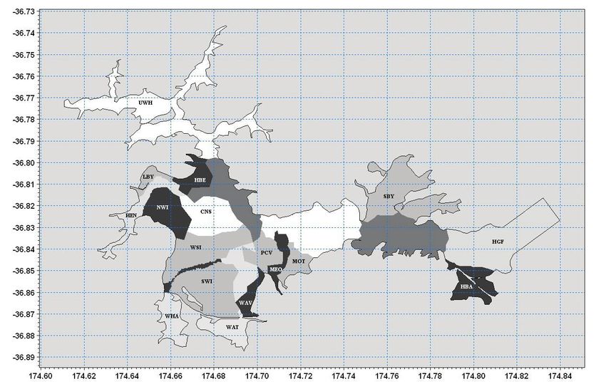
conducted for the Auckland Regional Council. The CWH was divided into 17 subestuaries (Fig. 4(a))
and the catchment was divided into 15 subcatchments. The CWH is a drowned-valley estuary that
receives drainage from the Upper Waitemata Harbour and opens to the east coast of the upper
North Island of New Zealand (Fig. 4(b)). It has a surface area of ~80 km2, and opens into the
Hauraki Gulf, which is sheltered from ocean waves. Two large embayments – Shoal Bay to the
north and Hobsons Bay to the south – open out from the throat of the harbour, which is crossed by
the Auckland Harbour Bridge. The main body of the harbour, to the west of the throat, comprises
tidal flats around the fringes, expanses of subtidal flats (to 5 m deep), deeper channels (10–15 m
deep) and tidal creeks (Whau River, Henderson Creek) that discharge along the southwestern
shore. The tide is semidiurnal with a range of 1–2 m, and the water column in the main body of the
harbour is typically well-mixed. The CWH receives runoff from a 205 km2 land catchment, about
half of which discharges via Henderson Creek. Even in flood, freshwater runoff through
Henderson Creek is insufficient to stratify the water column in the main body of the harbour. Bed
sediments in the main body typically contain less than 10% mud, and the median grainsize is 130–
170 μm. Bed sediments in the tidal creeks are finer.Predicting decadal-scale estuarine sedimentation for planning catchment development 555
UWH
(a)
HBE SBY
LBY
CNS
NWI HGF
HEN
WSI MOT
SWI MEO
PCV HBA
WHA WAT WAV
(b)
Fig. 4 (a) Subestuaries. (b) Location map.
USC model calibration against sedimentation data
The USC model was run for the historical period 1940–2001, with sediment inputs from the
catchment, hindcast by GLEAMS, appropriate to that period. The aim of the calibration process
was to adjust various terms in the USC model so that its hindcasts of sedimentation rate during the
historical period came to match observations from that same period. The main adjustment related
to the behaviour of “dynamic sinks” in the model, as follows.
The database of dispersal and deposition patterns (example patterns are shown in Figs 1–3)
describes, in effect, the strength and direction of sediment-transport pathways or “connections”
amongst subestuaries. These connections form a complex network, with multiple cross-connections
and interactions possible. The network of connections determines which parts of the estuary ultimately
accumulate sediments, which are termed here “dynamic sinks”, because they arise from the
behaviour of the system (cf. a static sink that would be created by, for instance, simply preventing
erosion in that part of the estuary). Any small errors associated with the connection strengths and
directions – which are determined by the DHI simulations – may interact and grow. This kind of
problem is unavoidable in any scheme that seeks to extrapolate error-prone calculations beyond the
scale at which the calculations are first performed. In the case of the USC model, we are attemp-
ting to scale-up patterns of sediment dispersal that apply at a roughly daily time scale to a final
time scale that is order 104 times larger than daily. If the Central Waitemata Harbour is primarily
dispersive, in the sense that sediments are passed more-or-less randomly in all directions amongst
subestuaries, then the growth of errors should be minimised. But, that notion cannot be entirely true,556 M. O. Green
since there obviously will be preferred sediment-transport routes. The goal in the calibration of the
USC model, which is obtained by relaxing and strengthening connections appropriately, is to get
all of the dynamic sinks in the model domain to simultaneously accumulate sediment at realistic rates.
By radioisotopic dating of sediment cores, Swales et al. (2007) determined an average
sedimentation rate over the past 50 years or so of 3.2 mm/year for intertidal sites in the Central
Waitemata Harbour (range 0.7–6.8 mm/year), and 3.3 mm/year for subtidal sites (range 2.2–5.3
mm/year). Sedimentation rates were more variable at intertidal sites compared to subtidal sites.
The USC hindcast sedimentation rates are generally smaller than the radioisotopic sedimentation
rates by about 25%; however, the patterns of sedimentation are similar in important respects, as
follows (refer to Fig. 5): (a) The hindcast sedimentation rates in Henderson Creek and the Whau
River (5.7 and 3.7 mm/year, respectively), which are both tidal creeks, exceeded the hindcast
sedimentation rates at all places outside of the tidal creeks. This concurs with previous obser-
vations of sedimentation in tidal creeks in the Auckland region (Swales et al., 2002). (b) The
largest hindcast sedimentation rate outside of the tidal creeks, with one exception, was in Shoal
Bay (2.2 mm/year). The largest radioisotopic sedimentation rate outside of the tidal creeks was
also in Shoal Bay. This is an interesting result, and is explainable by another observation, to be
described below. (c) The exception noted above is Limeburners Bay (3.3 mm/year). Limeburners
Bay may be viewed as an extension of Henderson Creek, from which sediments are primarily
received. (d) The hindcast sedimentation rates are smaller along the southern shore of the harbour
throat to the west of the Auckland Harbour Bridge compared to the intertidal flats in the main
body of the harbour further to the west. This is broadly in line with Swales et al.’s designation of
the southern shore as a “temporary sink”. (e) The hindcast sedimentation rates are smaller in the
subtidal flats in the main body of the harbour compared to the intertidal flats. The radioisotopic
data show the same pattern in at least one part of the main body of the harbour.
Patterns of sediment dispersal
A further reality check on the model performance is provided by examining patterns of sediment
dispersal, specifically the origins of sediments that deposit in each subestuary. For instance,
although sediments from all sources are generally well mixed together in the main body of the
harbour, deposition plumes are still traceable from respective subcatchment outlets. For instance,
Fig. 5 Hindcast sedimentation rates.Predicting decadal-scale estuarine sedimentation for planning catchment development 557
the northwestern intertidal flats are dominated by sediments deriving from the Henderson Creek
subcatchment, but the southwestern intertidal flats are dominated by sediments from the Whau
River subcatchment. Te Tokaroa Reef acts as a barrier to sediment dispersal, with sediments
discharged from subcatchments on either side of the reef prevented from mixing locally. With one
exception, sediments and metals that deposit in tidal creeks (Henderson Creek, Whau River) and
sheltered embayments (Limeburners Bay, Waterview Embayment, Hobsons Bay) are sourced from
the respective immediately adjacent subcatchment. Shoal Bay is the exception, which accumulates
sediments from every subcatchment except those that drain into the harbour on the southern shore
of the throat to the east of the Auckland Harbour Bridge. Some preliminary exploratory
simulations with the DHI model suite suggest that Shoal Bay siphons off suspended sediment
carried by ebb-tide flows through the harbour throat. This process is aided by an eddy that is shed
downstream on the ebb tide from Stokes Point (see Fig 4(b), this headland forms the western end
of the entrance to Shoal Bay). Sediments discharged from subcatchments that empty on the
southern shore of the throat to the east of the Bridge are not entrained in this eddy, which explains
why they do not accumulate in any significant quantity in Shoal Bay.
MODEL PREDICTIONS
The population in Auckland City is expected to increase significantly over the next 50 years. A
substantial part of the increased population will be housed by infill development, although there
are still greenfield areas in the region that may be developed. The Auckland Regional Council
contracted NIWA in 2005 to conduct the Central Waitemata Harbour Contaminant Study. The
main aim of the Study is to predict sedimentation and heavy metal (zinc, copper) accumulation in
the bed sediments of the Central Waitemata Harbour under a number of development scenarios
over the next 100 years (2001–2100) with a view to, amongst other things, identifying significant
sediment and metal sources, and testing the efficacy of different types of stormwater treatment and
options for controlling heavy-metal generation at source. The USC model was used to make the
predictions, which authorities are presently assessing. An interesting prediction regarding sedi-
mentation is shown here.
Catchment sediment runoff is predicted to decrease by about one-half over the next 100 years,
with most of the reduction occurring over the next 15–20 years as greenfield sites are exhausted
and development turns more towards infill. As a result of this, the predicted sedimentation rates in
the harbour are smaller, by one-third to two-thirds, than historical (past 50 years) sedimentation
rates. However, the decrease is not predicted to be uniform; in fact, the model predicts that
fundamental changes in depositional regime will result in some parts of the harbour.
The sedimentation rate is predicted to reduce in the main body of the harbour, as catchment
sediment runoff reduces (Fig. 6). For the tidal creeks, which are sinks, the sedimentation rate will
not be greatly affected. A possible explanation is related to a differential reduction in sediment
runoff, as follows. Given that much of the sediment runoff generated during larger rainfall events
is exported from the tidal creeks, and virtually all of the sediment runoff generated during smaller
rainfall events is deposited inside the tidal creeks (Fig. 1), then if sediment runoff during larger
events is reduced more than sediment runoff during smaller events, this would not necessarily
translate into a marked change in sedimentation rate.
8.0
Bed level increase (mm)
Main body of harbour
4.0 Southern shore of throat, west of Bridge
Tidal creeks
0.0
0 10 20 30 40 50 60 70 80 90 100
Years from 2001
Fig. 6 Predicted change in bed-sediment level, 2001–2100.558 M. O. Green
In contrast, subestuaries along the southern shore of the harbour throat, to the west of the
Auckland Harbour Bridge (see Fig. 5) are predicted to erode, for a time, as the catchment sediment
runoff reduces, and then reach a new transportational regime. Here, the reduction in sediment
runoff from the catchment effectively reduces sediment inputs to the point where they are matched
by erosion and removal of sediments (to other parts of the harbour) by waves and currents.
The predictions have important implications for the future accumulation of heavy metals in
the harbour bed sediments. Zinc and copper concentrations are predicted to rise continuously in the
tidal creeks, where sedimentation will remain virtually constant. For the main body of the harbour,
where the sedimentation rate is predicted to decline, the rise in heavy-metal concentrations will be
retarded. This occurs because physical and biological processes will be more effective at mixing
high-concentration sediment-metal inputs arriving from the land into the lower-concentration pre-
existing bed sediments under the reduced sedimentation rate. When the subestuaries in the harbour
throat become transportational, the metal concentrations there will stabilise. The stable
concentration will not really be an “equilibrium” concentration. Rather, it is more the case that
these subestuaries become “moribund” when deposition switches off.
CONCLUSIONS
The USC model combines information in physically-based ways from underlying models to make
predictions of estuarine sedimentation on the planning time scale, which is orders of magnitude
greater than typical estuary sediment-transport models. The model is proving to be a useful tool for
resource managers, since it makes explicit predictions about the future state of the environment
given certain management actions. The model also provides a comprehensive depiction of how
different parts of the estuary receiving waters are “connected” to different parts of the catchment,
which promotes catchment-scale thinking. Predictions for the Central Waitemata Harbour reveal a
complicated response to a reduction in catchment sediment runoff expected over the next 15–20
years, which has implications for the accumulation of heavy metals.
Acknowledgements This work has been funded by the Auckland Regional Council and the (New
Zealand) Foundation for Research, Science and Technology (C01X0307).
REFERENCES
Bottcher, A. B., Hiscock, J. G., Pickering, N. B. & Jacobsen, B. M. (1998) WAM: Watershed Assessment Model for
agricultural and urban landscapes. Proc. 7th International Conference of Computers in Agriculture (Orlando), 257–268.
ASAE Publication 13-98, St Joseph, Michigan, USA.
Cooper, A. B. & Bottcher, A. B. (1993) Basin scale modelling as a tool for water resource planning. J. Water Resour. Plan.
Manage. 119, 303–323.
Ellis, J., Cummings, V. J., Hewitt, J. E., Thrush, S. F. & Norkko, A. (2002) Determining effects of suspended sediment on
condition of a suspension feeding bivalve (Atrina zelandica): results of a survey, a laboratory experiment and a field
transplant experiment. J. Exp. Mar. Biol. Ecol. 267, 147–174.
Ellis, J. Nicholls, P., Craggs, R., Hofstra, D. & Hewitt, J. E. (2004) Effects of terrigenous sedimentation on mangrove
physiology and associated macrobenthic communities. Mar. Ecol. Progr. Ser. 270, 71–82.
Green, M. O. & MacDonald, I. M. (2001) Processes driving estuarine infilling by marine sands on an embayed coast. Mar.
Geol. 178, 11–37.
Green, M. O. & Coco, G. (2007) Sediment transport on an estuarine intertidal flat: measurements and conceptual model of
waves, rainfall and exchanges with a tidal creek. Est. Coastal Shelf Sci.72, 553–569.
Holthuijsen, L. H., Booij, N. & Ris, R. C. (1993) A spectral wave model for the coastal zone. Proc. 2nd Int. Symposium on
Ocean Wave Measurement and Analysis, New Orleans, USA, 630–641.
Hume, T. M. & McGlone, M. S. (1986) Sedimentation patterns and catchment use change recorded in the sediments of a
shallow tidal creek, Lucas Creek, Upper Waitemata Harbour, New Zealand. New Zealand J. Mar. Freshw. Res. 20, 677–687.
Knisel, W. G. & Davis, F. M. (2000) Groundwater Loading Effects of Agricultural Management Systems, Version 3.0.
Publication no. SEWRL-WGK/FMD-050199, revised 081500. Washington, USA.
Lohrer, A. M., Thrush, S. F., Hewitt, J. E., Berkenbusch, K., Ahrens, M. & Cummings, V. J. (2004) Terrestrially derived
sediment: response of macrobenthic communities to thin terrigenous deposits. Mar. Eco. Progr. Ser. 273, 121–138.
Swales, A., Williamson, R. B., van Dam, L. F., Stroud, M. J. & McGlone, M. S. (2002). Reconstruction of urban stormwater
contamination of an estuary using catchment history and sediment profile dating. Estuaries 25(1), 43–56.
Swales, A., Stephens, S., Hewitt, J. E. Ovenden, R., Hailes, S., Lohrer, D., Hermansphan, N., Hart, C., Budd, R., Wadhwa, S. &
Okey, M. (2007) Central Waitemata Harbour Study. Harbour Sediments. NIWA Client Report HAM2007-001.You can also read